Time Series RUL Estimation of Medium Voltage Connectors to Ease Predictive Maintenance Plans


1
Electronics Engineering Department, Universitat Politècnica de Catalunya, 08222 Terrassa, Spain
2
Electrical Engineering Department, Universitat Politècnica de Catalunya, 08222 Terrassa, Spain
*
Author to whom correspondence should be addressed.
Appl. Sci. 2020, 10(24), 9041; https://0-doi-org.brum.beds.ac.uk/10.3390/app10249041
Submission received: 9 November 2020
/
Revised: 12 December 2020
/
Accepted: 15 December 2020
/
Published: 17 December 2020
(This article belongs to the Special Issue Reliability Techniques in Industrial Design)
Abstract
:The ageing process of medium voltage power connectors can lead to important power system faults. An on-line prediction of the remaining useful life (RUL) is a convenient strategy to prevent such failures, thus easing the application of predictive maintenance plans. The electrical resistance of the connector is the most widely used health indicator for condition monitoring and RUL prediction, even though its measurement is a challenging task because of its low value, which typically falls in the range of a few micro-ohms. At the present time, the RUL of power connectors is not estimated, since their electrical parameters are not monitored because medium voltage connectors are considered cheap and secondary devices in power systems, despite they play a critical role, so their failure can lead to important power flow interruptions with the consequent safety risks and economic losses. Therefore, there is an imperious need to develop on-line RUL prediction strategies. This paper develops an on-line method to solve this issue, by predicting the RUL of medium voltage connectors based on the degradation trajectory of the electrical resistance, which is characterized by analyzing the electrical resistance time series data by means of the autoregressive integrated moving average (ARIMA) method. The approach proposed in this paper allows applying predictive maintenance plans, since the RUL enables determining when the power connector must be replaced by a new one. Experimental results obtained from several connectors illustrate the feasibility and accuracy of the proposed approach for an on-line RUL prediction of power connectors.
1. Introduction
Power connectors are widely used in transmission and distribution grids. Although power connectors are simple elements, they are often placed in critical links, thus playing a key role for the reliable, stable, and long-term operation of power systems. However, like in many other power devices, their performance tends to degrade progressively during the operating condition [1], which may result in power system failures, sometimes with catastrophic and costly effects [2]. The expected lifetime of power connectors under continuous operation is several years, but the occurrence of premature faults can shorten this period [3]. Therefore, there is an imperious need to develop strategies to analyze the degradation process of power connectors, while predicting their RUL, i.e., the estimated operating time before the connector must be replaced. Remaining Useful Life (RUL’s) accurate prediction enables effective maintenance strategies to be applied by anticipating when connectors will be replaced, thereby minimizing the risk of premature failure and the associated unwanted effects [4]. This is an issue for power utilities and system operators, as they go to great lengths to ensure a reliable, uninterrupted, and safe power delivery to their customers [5].
Medium voltage connectors are predominantly made of aluminum or copper [6], usually of compressed type, and designed to guarantee steady and reliable electrical connections between two bus bars or conductors with reduced voltage drop and power loss [7,8].
It is a recognized fact that the electrical resistance of the electrical connectors plays a key role on the correct behavior of the connectors [9]. The electrical resistance has two main components, i.e., the bulk and the contact resistance. The bulk resistance is determined by the geometry of the connector and the electrical conductivity of its constitutive materials, whereas the contact resistance depends on several factors including the state, the roughness, and the pressure of the contact interfaces as well as the presence of debris and dirt. The degradation of the connector is reflected in an increase in its electrical resistance, which tends to increase the working temperature. It overheats the connector, which, in turn, increases the electrical resistance, thus shortening the expected life [9]. Different causes such as poor installation or the daily peak and off-peak temperature cycles, which generate contraction and expansion patterns, tend to loosen the contact, thus increasing the contact resistance. When the electrical resistance surpasses a limit value, the connector must be replaced to avoid possible hot spots and failures. Electrical resistance is the most critical parameter to determine the health status of power connectors, which tends to increase over time [10], since the different degradation mechanisms tend to produce negative effects on contact resistance, thus affecting negatively the electrical and thermal performances of the connectors. Therefore, the electrical resistance can be effectively used to predict the RUL of such devices.
Although RUL strategies are much needed, the information found in the technical literature about RUL prediction methods for power connectors is scarce, in particular, when considering realistic operating conditions. The joint effect of temperature and vibrations on the resistance of automotive connectors was evaluated in [10], whereas in [11], the fatigue lifespan of microconnectors was studied. The effects of vibrations in the RUL of aviation connectors were evaluated in [12] by applying a particle filtering-based method and accelerated degradation tests (ADTs). ADTs were also applied in [13] to determine the failure rate and reliability of electrical connectors when subjected to temperature and particulate contamination stresses. In [14], the lifetime distribution of circular electrical connectors was approximated by a parametric Weibull distribution, its parameters being identified from degradation data. In [15], the RUL of microswitches was estimated by applying different methods, including Bayesian updating, expectation maximization, and strong tracking filtering [15]. In [16], the RUL of socket connectors was determined by analyzing the change in the resistance.
ADTs are often applied to determine long-term effects of expected stress levels [17] by investing a shorter time. Many authors predict the RUL from the analysis of experimental data acquired from ADTs [12,18,19] to predict the long-term behavior of the analyzed devices. Although ADTs can generate reliable data, they are costly in terms of invested time, hours spent by technician, energy consumption and consumed materials. In addition, the obtained data are often specific of the tested sample, so they suffer from the lack of generalizability.
RUL prediction is mainly based on four approaches, i.e., model-based, data-driven, fusion-based, and hybrid models. According to [1,20], data-based RUL approaches usually provide superior on-line predictive performance than model-based approaches, although the accuracy of such approach can be enhanced by applying a fusion strategy based on combining different data-driven algorithms. Hybrid strategies combine model-based and data-driven algorithms, thus taking advantage of the benefits of both approaches. Model-based approaches or white-box models are based on describing the physics of the analyzed system and its failure modes using a set of mathematical equations, so this approach does not require historical performance data. Data-driven or black-box approaches progressively learn the behavior of the studied system directly from the collected data. This approach assumes that system data presents a reasonably deterministic statistical behavior of the system, unless it operates under fault conditions. Since data-driven approaches methods rely on collected data, they can predict the behavior of the system in the near future and especially at the end of its useful life due to the amount of data acquired [20]. Data-driven approaches include methods based on time-series, statistical, and artificial intelligence.
It is possible to predict the degradation of power connectors by analyzing the degradation trajectory, which can be effectively applied to determine the RUL. It requires identifying the most influencing degradation factors and their influence in the prediction process. Although the analysis of the degradation trajectory is gaining attention, there is still little research in this area [21], and thus, a precise RUL prediction from the degradation trajectory is a challenging task.
This paper develops a quite simple method based on an on-line acquisition of the voltage drop, electric current, and temperature of power connectors, so that these data are used to determine the degradation trajectory of the electrical resistance, which is the baseline to determine the RUL. The RUL is inferred by applying a fast and simple approach based on the autoregressive integrated moving average (ARIMA) method [22], which is based on actual and past values of the electrical resistance of the connectors. This paper contributes in different ways. First, it deals with the RUL of power connectors, an area requiring more research works. Second, the method proposed in this work has superior capabilities with respect to other methods found in the technical literature, since it is simple, fast, and easy to apply, so that the acquired data can be processed in low-power inexpensive microcontrollers that in a near future will be integrated into the power connectors for an on-line RUL prediction. Third, this approach is fully aligned with digital substations, smart grids, and Internet of Things (IoT), where predictive maintenance, RUL, and fault diagnosis are hot topics, and nowadays, power connectors are still far from these trends. Fourth, the approach proposed in this paper avoids the application of accelerated degradation tests (ADTs), which are costly and often lack generalizability. Fifth, this approach can be applied to different power components, such as electromechanical contactors or relays among others.
The rest of the paper is organized as follows. Section 2 emphasizes that electrical resistance is a good indicator of connector health, as well as how it can be measured indirectly. Section 3 explains the adopted RUL criterion in this work based on resistance degradation trajectory and a pre-established threshold. The ARIMA models and their variants are discussed in Section 4. Section 5 presents the experimental setup used to carry out the experimental measurements of connector degradation, while Section 6 presents the obtained results attaining the RUL prediction according to various ARIMA models. Finally, Section 7 summarizes and concludes the paper.
2. The Role of the Electrical Resistance on Ageing
The electrical resistance is known to play an important role on the degradation of power connectors [23], being an excellent indicator of their health condition [24]. Any rise of the electrical resistance is translated in an increase of the connector’s operating temperature, which further rises the electrical resistance, thus degrading the thermal behavior of the connector and reducing its expected useful life [3].
Despite its importance, it is not possible to measure electrical resistance directly, so indirect methods are required. The common method to measure the electrical resistance is by measuring the voltage drop across the connector terminals and the electrical current circulating in the connector. However, this method is valid in direct current (DC) circuits but it cannot be applied directly in alternating current (AC) circuits, since under AC supply, the impedance of the connector ZC is obtained instead of the resistance,
where ∆Vt,T is the instantaneous value of the voltage drop across the terminals of the connector measured at time t when its temperature is T, and It is the instantaneous value of the current flowing in the connector at the same time t. It is noted that for an on-line monitoring of the resistance of the connector, It is the AC current flowing in the loop or installation where the connector is placed.
In order to determine the electrical resistance of the connector, the phase shift between the voltage drop and the current waveforms must be measured. It can be done by applying the properties of the phasors as,
where Rt,T and Xt,T are, respectively, the instantaneous values of the resistance and the reactance of the connector, and φ is the phase shift between the voltage drop and the current waveforms.
It is known that the electrical resistance changes with the temperature of the connector, so this effect has to be considered in the measurements. To deal with the effect of temperature, the resistance of the connector is often referred to 20 °C (Rt,20 °C) and thus from (2),
where α is the coefficient of temperature coefficient, its value being around 0.004 °C−1 for pure aluminum and copper materials.
As mentioned before, the electrical resistance of medium-voltage connectors is in the range of a few micro-ohms, and thus, special care must be taken when measuring this magnitude.
3. The RUL Criterion
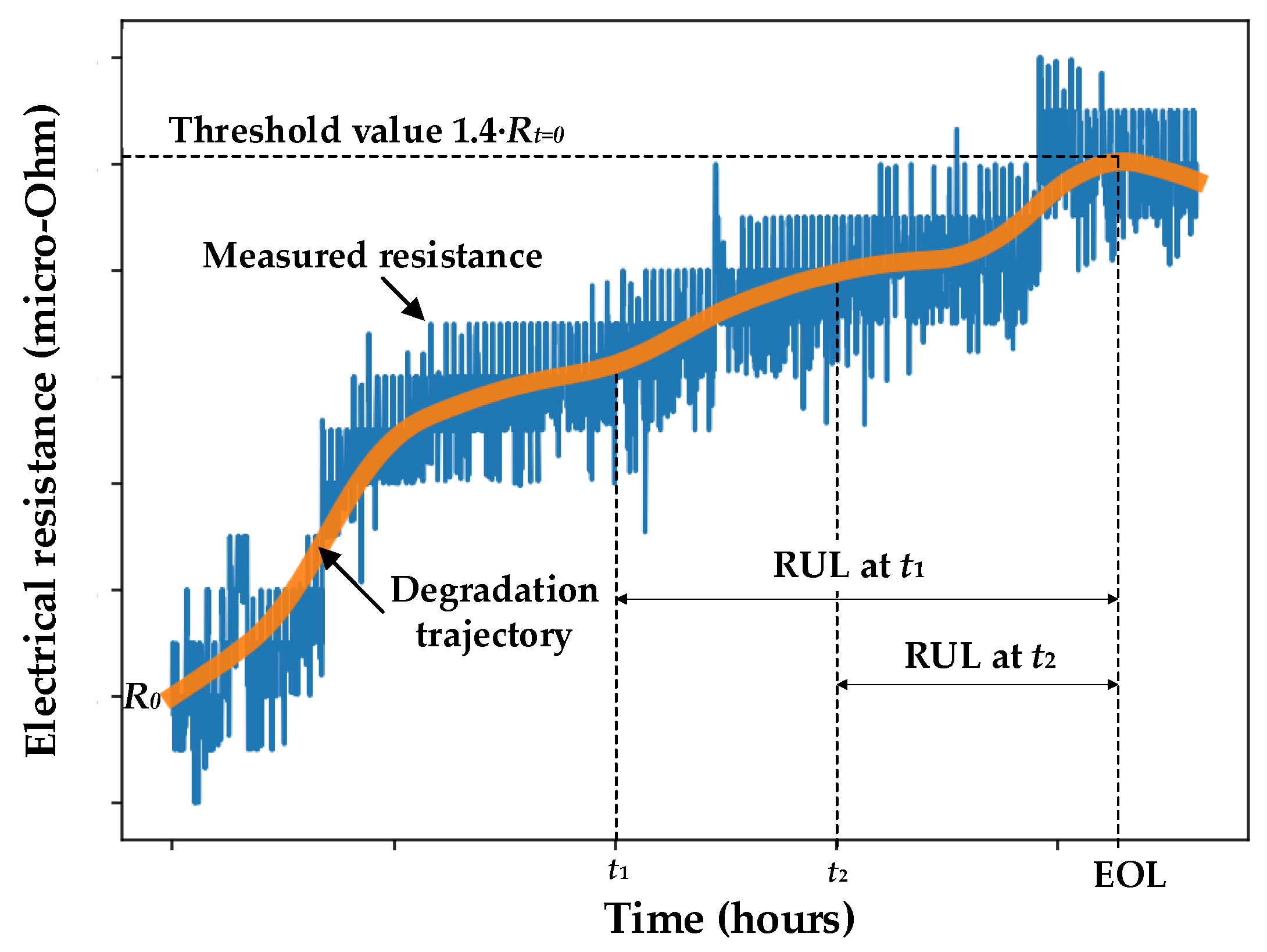
The RUL is defined as the time interval from the present moment until the connector reaches the end-of-life (EOL). The EOL indicates that the conductor has reached the end of its useful life, so it must be replaced by a new one because its thermal and electrical behaviors are below predefined levels. Therefore, a simple and unambiguous criterion to determine the EOL, and thus the RUL, is required. In this work, it is assumed that the EOL is attained when the resistance of the connector is increased by at least 40% with respect to its initial value Rt = 0, i.e., the RUL is the time interval between the current instant and the time in which the connectors resistance is 1.4·Rt = 0. The 40% resistance increase corresponds to a limit value that takes into account an increase in power losses by 40% and a sufficient temperature rise to age the connector.
Figure 1 shows how to determine the EOL and thus the RUL.
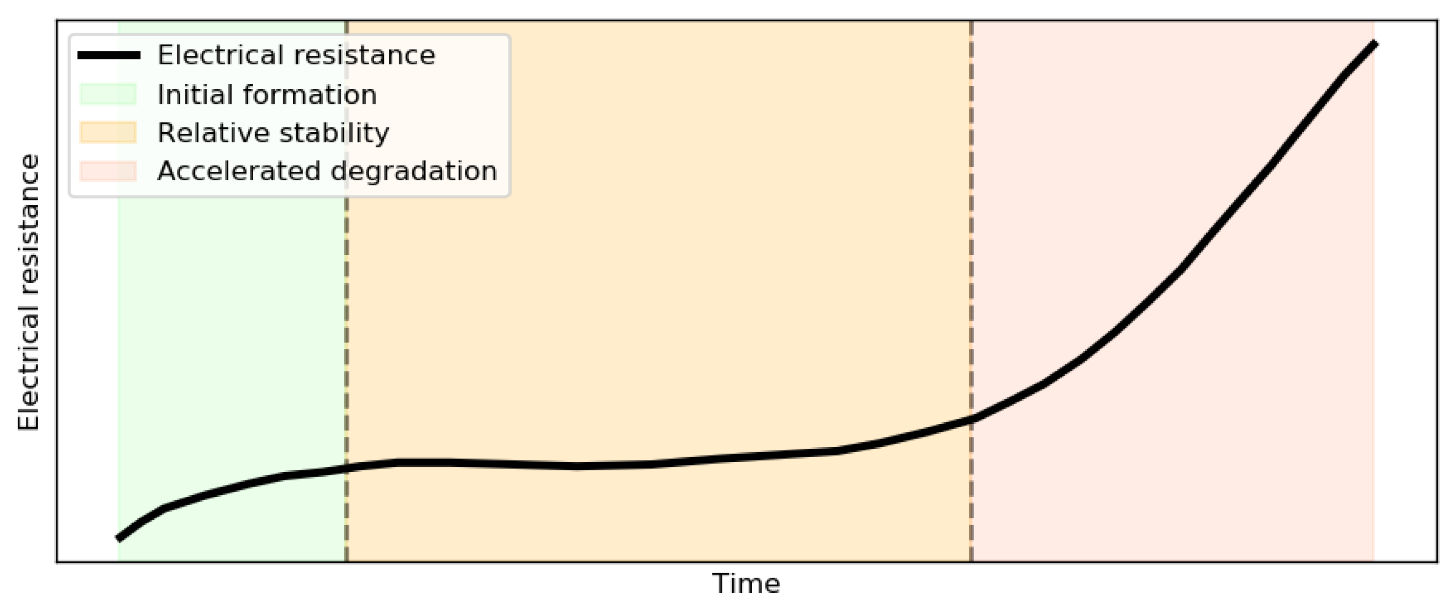
The expected evolution of the resistance of the connector according to the IEC 61238-1-1 international standard [25] corresponds to a monotonic increase of resistance (see Figure 2), where three main stages are described. The first stage is known as initial formation region, where the resistance experiments an initial change just after the installation of the connector, during which stable constriction areas are stablished. This stage is followed by a relative stability region in which its resistance is almost constant. Finally, in the last stage, known as accelerated ageing or degradation, the resistance experiments a fast change because the connector is reaching its EOL.
4. The Autoregressive Integrated Moving Average (ARIMA) Approach for RUL Prediction
The ARIMA model was developed by Box and Jenkins in 1970 [22]. The projections generated by means of the ARIMA model can be understood as the integration of the latest observations combined with the long-term historical tendency [26], being an intuitively reasonable model to describe many practical time series [22]. ARIMA is a type of time-domain model that is often used to fit and forecast time series that exhibit temporal correlation. ARIMA models have been applied to forecast time series of climate-related variables [26], economic variables [27], or pandemics [28], as well as to determine the RUL of batteries [1] and aircraft engines [29], among many other applications. ARIMA models are suitable to describe both stationary and nonstationary time series data. The properties of stationary time series are independent of the observation time, so the time series that present seasonality or trends are nonstationary, since seasonality and trend influence the time series at different times. However, cyclic time series without trend or seasonality are stationary. ARIMA models are based on autoregressive (AR), moving average (MA), and autoregressive moving average (ARMA) models [1].
ARIMA models take into account a linear combination of the current value, past values, nonseasonal differences, and lagged forecast errors of a time series degradation data for predicting the future response. The differences are used for removing nonstationarity, since stationary time series do not depend on the observation time. The AR or autoregressive term represents the regression variable based on the past values, whereas the MA or moving average term performs a linear combination of the regression errors [20].
The AR(p) model of order p can be viewed as a discrete set of time-lags linear equations,
where Rt and denote the measured and predicted values of the electrical resistance at time t, respectively.
The MA (q) term of order q can be expressed as,
where the error terms are given by,
When neglecting the nonseasonal difference terms with order d, the ARIMA (p,0,q) is obtained, which, in fact, is an ARMA (p,q) model, which can be described as,
A nonseasonal ARIMA (p,d,q) model includes p autoregressive terms, d nonseasonal differences, and q lagged forecast errors. The ARIMA (p,d,q) is as an ARMA (p,q) model of , that is,
where , and L is the lag operator, i.e., LRt = Rt−1 and LdRt = Rt−d, so Rt is obtained from by performing d successive integrations.
Therefore, ARIMA models can be understood as an improved version of ARMA models, which are suitable for stationary and nonstationary time series. In the case of nonstationary time series, the d-order nonseasonal differences terms are required to convert nonstationary into stationary time series. It is noted that in most applications, d is 0 or 1 [1]. The ARIMA (p,d,q) problem consists of determining the αi and γj coefficients from the time series data of . It results in a fitting and optimization problem, whose solution requires to determine the minimum value of an objective function, which is calculated from,
where n is the number of terms of the training data, so the objective function becomes,
To minimize the objective function f, the free derivative Nelder–Mead algorithm [30], also known as downhill simplex method is used, which provides the optimum values of the αi and γj coefficients. This algorithm requires an initial seed values of such coefficients, which in this case has been settled to an arbitrary value of 0.1.
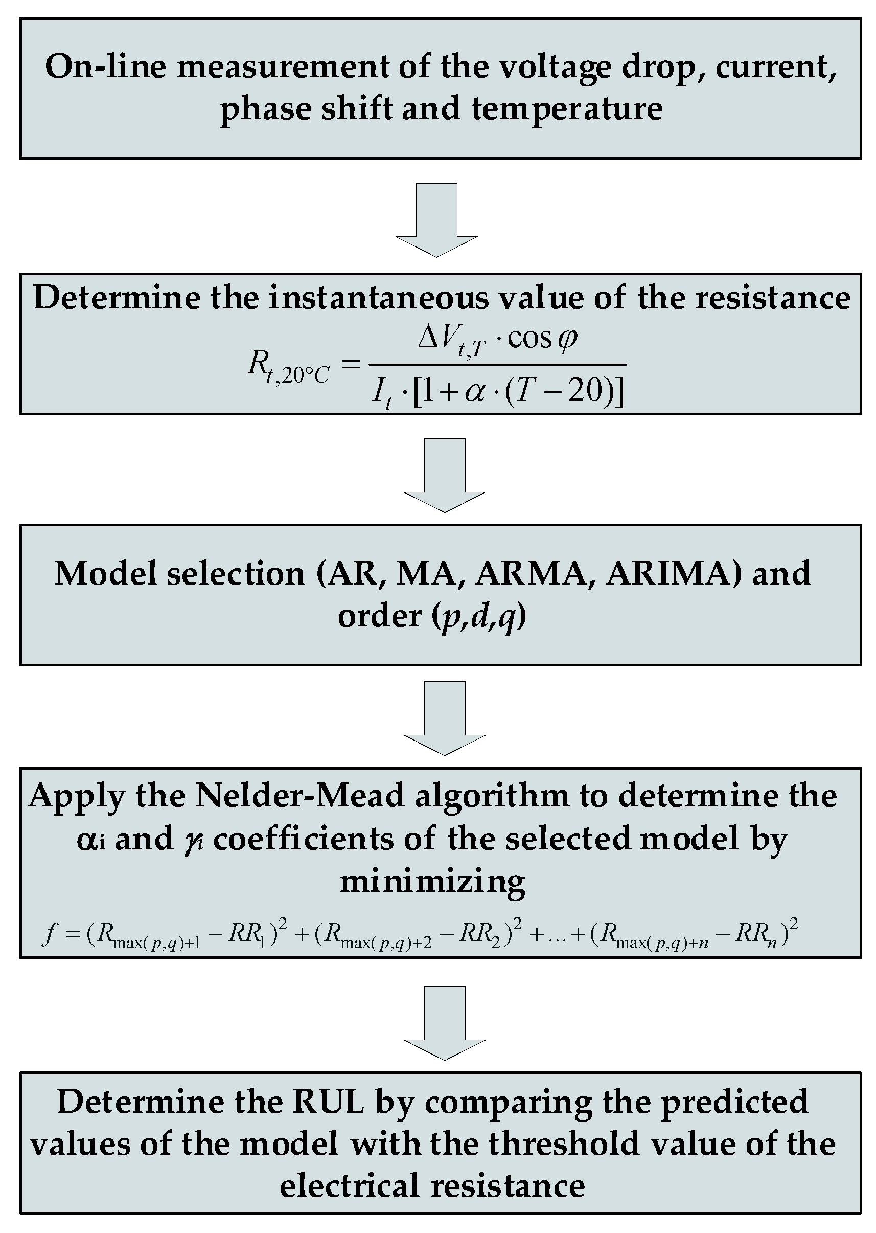
Figure 3 summarizes the strategy proposed in this work to determine the RUL of each connector. It is worth noting that each connector has its own behavior, so each one has its particular model, also depending on the instant in which it is trained to infer the RUL.
5. Experimental Setup and Historical Data Acquisition to Validate the Models
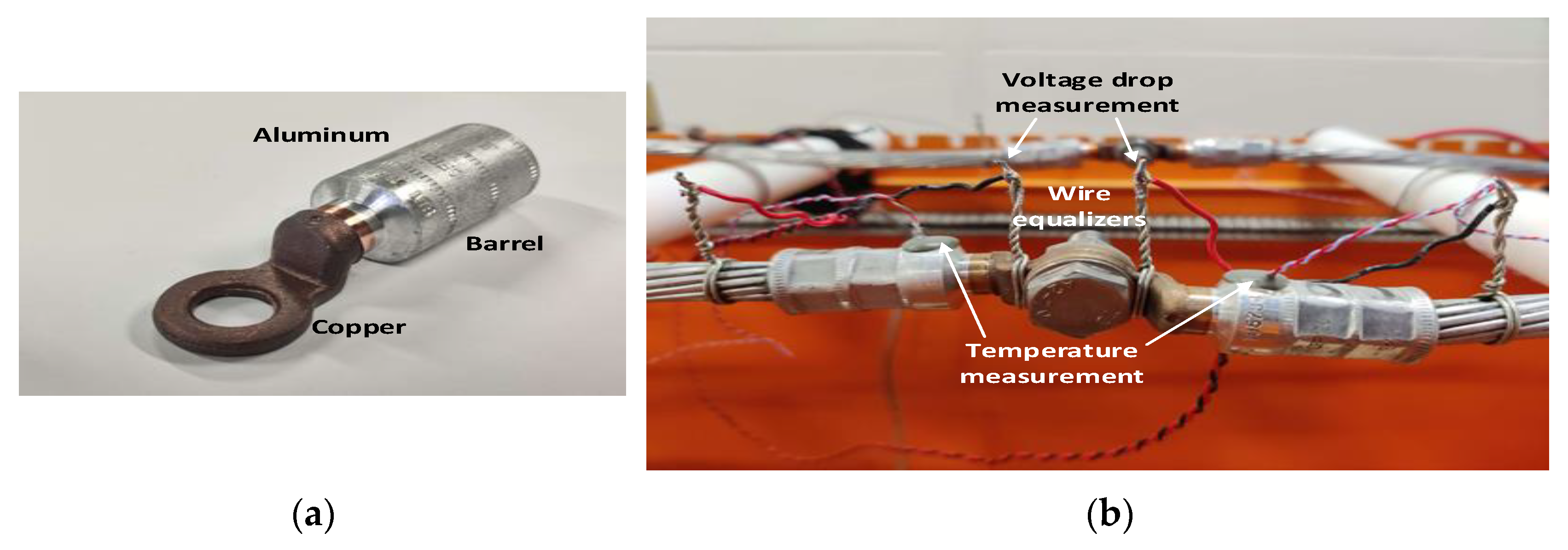
This paper analyzes the behavior of seven bimetallic friction-welded medium-voltage connectors of the same model (ICAU120 from the catalogue of SBI Connectors). These connectors are of Class B according to IEC 61238-1-3:2018 standard [25]. Figure 4a shows one of the connectors before being compressed to the conductor. The connectors are made of copper and aluminum and are designed to be connected to 120 mm2 aluminum stranded conductors. During installation, the stranded conductors are crimped within the aluminum barrels of the connectors [31] using an hexagonal crimping tool, model BURNDI Y35-BH EP-1HP (max compression force 120 kN) (Manchester, UK) with a remote compression head of 120 kN force. The current loop used in this work has been created by bolting the connectors to each other using M10 bolts, which were tightened by applying a torque of 35 Nm. It is noted that to minimize the contact resistance between the stranded conductor and the aluminum barrel of the connector, the internal part of the barrel is filled with a contact grease that withstands 140 °C.
The final objective of this research work is to determine the RUL of substation connectors, since they are often placed on critical points of the substations, and thus, failure of a substation connector can lead to costly and severe consequences. However, due do their size and rated current, the tests needed to acquire historical data require more time, power, and energy than when using medium-voltage connectors. Therefore, the results obtained with the medium-voltage connectors studied in this work will be used to validate the proposed approach, which latter will be applied to the substation connectors.
In a final application, the data (voltage drop, current and temperature) will be acquired on-line in the field, i.e., at the location where the connector is installed. In this work, the data is acquired in the AMBER high-voltage and high-current laboratory of the Universitat Politècnica de Catalunya.
To acquire degradation data and to characterize the thermal and electrical behavior of the seven analyzed connectors, they were subjected to heat cycle tests following the procedure detailed in the IEC 61238-1-3:2018 standard [25]. Heat cycle tests are used to expedite the degradation process due to thermal ageing [32]. In this work, the heat cycles are a means of collecting experimental data to validate the accuracy and appropriateness of the proposed RUL approach. For such tests, the connectors are fitted on stranded aluminum conductors as shown in Figure 4b. Equalizers are used in the test loop to ensure a point of equipotential in the stranded conductor, so that the voltage drop can be measured over a specific distance. Each heat cycle consists of a heating and a cooling phase, thus producing thermal expansion and contraction effects, respectively, on the conductor and connectors, these effects have a non-negligible impact on the contact resistance, thus affecting the thermal and electrical behavior of the connectors. During the heating phase, an AC electric current is forced to flow through the loop to the point where the reference conductor temperature is 120 °C at thermal equilibrium. This condition was achieved by circulating an electrical current in the range of 350–380 ARMS. Once the equilibrium was reached, this elevated current was maintained during 15 min as described in the IEC 61238-1-3:2018 standard. The loop was then disconnected from the output of the high-current transformer to cool it by forced ventilation to room temperature. Then, the next heat cycle was started. A total of 140 heat cycles were performed during 92.5 h. It is noted that recommended operating temperature of the 120 mm2 aluminum stranded conductor is below 90 °C, and thus, the degradation process was accelerated by forcing the conductor to withstand 120 °C.
During the heat cycle tests, the voltage drop, current, and temperature of the connectors were measured every 6 s to calculate their electrical resistance, thus being possible to determine the degradation trajectory of the electrical resistance, which describes the evolution of electrical resistance over time.
A data acquisition (DAQ) device from National Instruments (NI USB-6210, 8 differential inputs, 88 μV absolute resolution) (Austin, Texas, United States) was used to measure the voltage drop waveforms across of the seven connectors. A calibrated CWT Rogowski coil (CWT500LFxB, 0.06 mV/A sensitivity) was used to measure the electric current, which was connected to one of the differential inputs of the DAQ. Both the current waveforms and voltage drop were sampled at a frequency of 5 kSamples/s during a few periods every 6 s. T-type thermocouples connected to an Omega Thermocouple Data Logger (USB TC-08, 8 channel, up to 10 measurements/s) were used to measure the temperature of the stranded conductor and the medium-voltage connectors, obtaining a temperature accuracy better than 1 °C. The accuracy in measuring the electrical resistance with this setup is better than 1 μΩ.
6. Results
This section evaluates the behavior and accuracy of the proposed approach for estimating the RUL based on the experimental results carried out in the electrical loop, including the seven analyzed connectors. The experimental results were obtained by means of the accelerated degradation process induced by the heat cycle tests detailed in Section 5.
After running several models, some conclusions can be stated. First, in this problem the inclusion of the I or integral term makes the results poorer, because the prediction that is based only on the finite differences (of order d) of the measured instantaneous resistance does not provide useful information to the model. Therefore, for the presented case study, ARMA models present better performances compared to the ARIMA models. Second, the AR term is always required, and the MA term can help to improve the performance of the AR part.
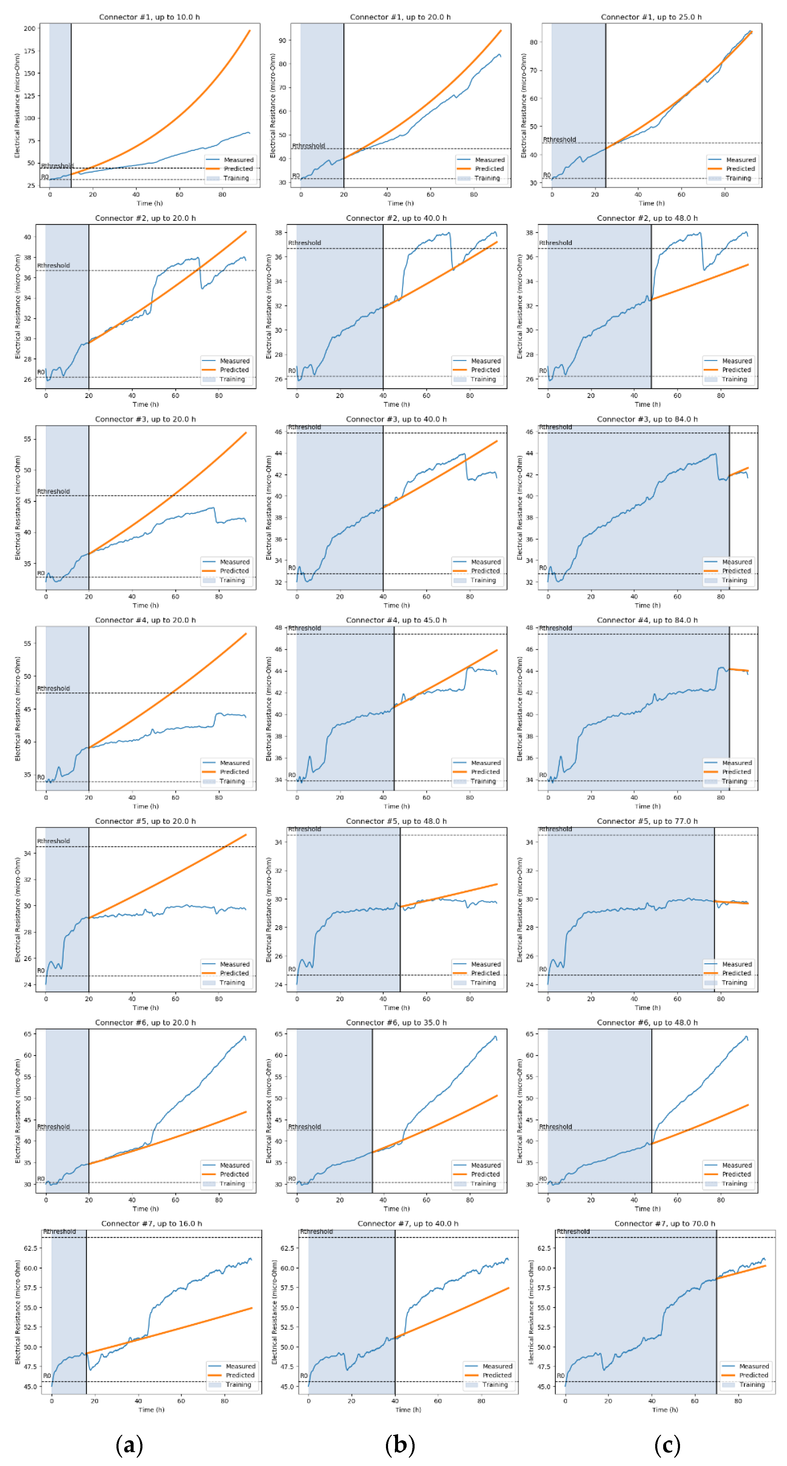
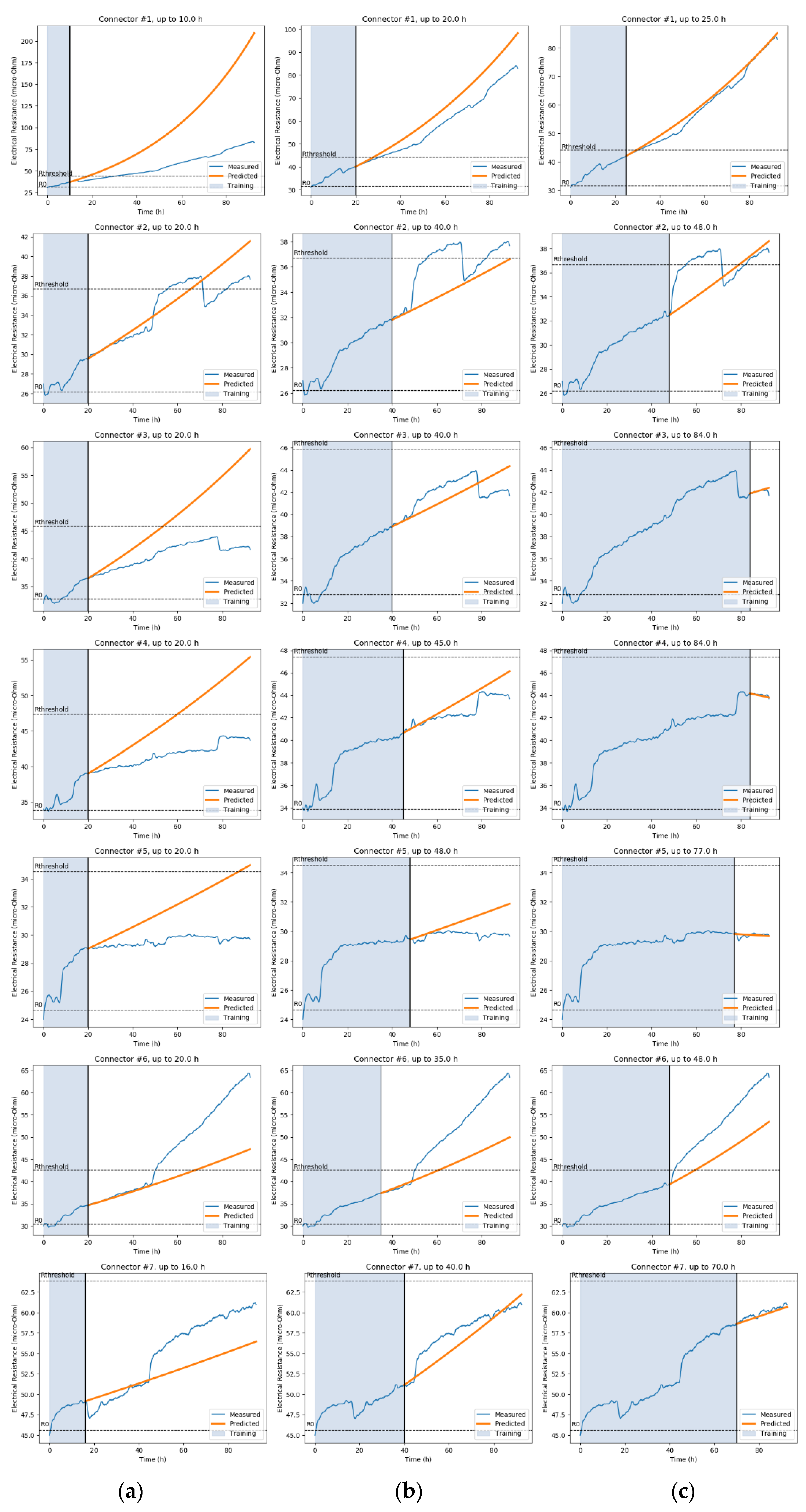
Table 1 shows the estimated RUL for the 7 considered electrical connectors when fitted by means of the AR (p = 3) and ARMA (p = 2, q = 2) models, as formulated in (4) and (8), respectively. Each of the columns corresponds to a different time horizon, for which the training stage of the model and the forward RUL estimation has been carried out. The RUL of each connector has been inferred in three different instants of time, which are summarized in Table 2. Note that not all the analyzed connectors have reached their EOL in the degradation experiment.
The AR (3) with p = 3 and the ARMA (2,2) with p = 2 and q = 2 have been revealed as the most reliable and adequate modes combining both ease of use in terms of computational efficiency as well RUL estimation accuracy.
Figure 5 and Figure 6 show, respectively, the results regarding the AR (3) and the ARMA (2,2) models, which consider 500 past data points, accounting for the last 4 h of past data. Each of the seven rows in Figure 5 and Figure 6 correspond to each of the seven studied connectors, whereas the three columns correspond to different time horizons. According to the observed degradation trajectory of the resistance for each connector, three prediction instants have been defined, as summarized in Table 2. The graphs in the first column take into account the last 4 h of data acquired between time 0 and time instant #1, so that the predictions made by the ARIMA model are solely based on the resistance measurements made from time 0 up to time instant #1 (blue area of the plots). The same applies for the remaining two columns of graphs in Figure 5 and Figure 6, which consider different final time instants. These graphs show the measured resistance between time 0 and the final time instant of the analyzed interval (blue line inside the blue area) as well as the predicted or future values of the resistance (orange line). Therefore, the fitting algorithm only considers the last 4 h of data available between time 0 and the final time instant of the analyzed interval. The predicted resistance trajectory (orange line) along several time horizons presented in Figure 5 and Figure 6 is of crucial importance to show the RUL estimation potential of the studied models.
As seen in Figure 5 and Figure 6, both models present a similar performance, and in general, their accuracy increases with the amount of available past data. It is observed that the resistance of the connectors sometimes undergoes sudden and unexpected changes, which makes its prediction extremely difficult by any mathematical algorithm.
Each of the RUL training/estimation calculation steps has been carried out, on average, in 1.1 s using an Intel i5-3470 CPU @ 3.20 GHz (Mountain View, California, USA) with 8 Gb of random access memory (RAM).
7. Conclusions
This paper has proposed an on-line approach to predict the remaining useful life (RUL) of power connectors, intended to ease and simplify the application of predictive maintenance plans. This simple on-line strategy, while presenting a reduced computational burden, allows forecasting the electrical behavior of the connector, thus enabling planning when the connector needs to be replaced because it has reached its end-of-life (EOL). The proposed strategy is based on monitoring the electrical resistance of the connectors, since it is a reliable indicator of their health condition. The proposed method predicts the RUL of the connectors based on the degradation path of the electrical resistance. The RUL of power connectors is determined by applying the autoregressive integrated moving average (ARIMA) method to the electrical resistance time series data. From experimental results based on heat cycle tests, which were used to force an accelerated degradation of the connectors, it has been shown that both AR (autoregressive) and ARMA (autoregressive moving average) models offer both simplicity and accuracy in predicting the RUL of the power connectors. Although accelerated ageing tests were performed to acquire reliable degradation data, in a real application, they are not required because the proposed method is based on the on-line data acquired for each connector. In addition, the RUL calculated by the proposed method is adapted to each particular connector, because it only considers the time series data of the particularly analyzed connector.
Author Contributions
Conceptualization, J.-R.R. and Á.G.-P.; methodology, J.-R.R.; formal analysis, M.M.-E. and Á.G.-P.; investigation, J.-R.R. and Á.G.-P.; writing—original draft preparation, J.-R.R.; writing—review and editing, M.M.-E. and Á.G.-P. All authors have read and agreed to the published version of the manuscript.
Funding
This research was partially funded by the Ministerio de Ciencia, Innovación y Universidades de España, grant number RTC-2017-6297-3, and by the Generalitat de Catalunya, grant number 2017 SGR 967.
Conflicts of Interest
The authors declare no conflict of interest.
References
- Chen, L.; Xu, L.; Zhou, Y. Novel Approach for Lithium-Ion Battery On-Line Remaining Useful Life Prediction Based on Permutation Entropy. Energies 2018, 11, 820. [Google Scholar] [CrossRef] [Green Version]
- Capelli, F.; Riba, J.-R.; Sanllehí, J. Finite element analysis to predict temperature rise tests in high-capacity substation connectors. IET Gener. Transm. Distrib. 2017, 11, 2283–2291. [Google Scholar] [CrossRef] [Green Version]
- Capelli, F.; Riba, J.-R.; Ruperez, E.; Sanllehi, J. A Genetic-Algorithm-Optimized Fractal Model to Predict the Constriction Resistance from Surface Roughness Measurements. IEEE Trans. Instrum. Meas. 2017, 66, 2437–2447. [Google Scholar] [CrossRef] [Green Version]
- Slade, P.G. Electrical Contacts: Principles and Applications, 2nd ed.; CRC Press: Boca Raton, FL, USA, 2017. [Google Scholar]
- De Paulis, F.; Olivieri, C.; Orlandi, A.; Giannuzzi, G. Detectability of Degraded Joint Discontinuities in HV Power Lines Through TDR-Like Remote Monitoring. IEEE Trans. Instrum. Meas. 2016, 65, 2725–2733. [Google Scholar] [CrossRef]
- Kadechkar, A.; Moreno-Eguilaz, M.; Riba, J.-R.; Capelli, F. Low-Cost Online Contact Resistance Measurement of Power Connectors to Ease Predictive Maintenance. IEEE Trans. Instrum. Meas. 2019, 68, 4825–4833. [Google Scholar] [CrossRef]
- Carvou, E.; El Abdi, R.; Razafiarivelo, J.; Ben Jemaa, N.; Zindine, E.M. Thermo-mechanical study of a power connector. Measurement 2012, 45, 889–896. [Google Scholar] [CrossRef]
- Pascucci, V.; Ryan, A.; Martinson, B.; Hsu, I.; Dandl, C.; Conde, P.; Chan, B.; Kirkbride, S. A Standardized Reliability Evaluation Framework for Connections. In SMTA International; SMTA: Rosemont, IL, USA, 2016; pp. 1–10. [Google Scholar]
- Riba, J.-R.; Mancini, A.-G.; Abomailek, C.; Capelli, F. A 3D-FEM-based model to predict the electrical constriction resistance of compressed contacts. Measurement 2018, 114, 44–50. [Google Scholar] [CrossRef]
- El Abdi, R.; Carvou, E.; Benjemâa, N. Electrical resistance change of automotive connectors submitted to vibrations and temperature. In 2015 IEEE Energy Conversion Congress and Exposition (ECCE); Institute of Electrical and Electronics Engineers (IEEE): Piscataway, NJ, USA, 2015; pp. 1910–1913. [Google Scholar]
- Huang, B.; Li, X.; Zeng, Z.; Chen, N. Mechanical behavior and fatigue life estimation on fretting wear for micro-rectangular electrical connector. Microelectron. Reliab. 2016, 66, 106–112. [Google Scholar] [CrossRef]
- Sun, B.; Li, Y.; Wang, Z.; Ren, Y.; Feng, Q.; Yang, D.; Lu, M.; Chen, X. Remaining useful life prediction of aviation circular electrical connectors using vibration-induced physical model and particle filtering method. Microelectron. Reliab. 2019, 92, 114–122. [Google Scholar] [CrossRef]
- Qingya, L.; Jinchun, G.; Gang, X.; Qiuyan, J.; Rui, J. Lifetime prediction of electrical connectors under multiple environment stresses of temperature and particulate contamination. J. China Univ. Posts Telecommun. 2016, 23, 61–81. [Google Scholar] [CrossRef]
- Ren, Y.; Feng, Q.; Ye, T.; Sun, B. A Novel Model of Reliability Assessment for Circular Electrical Connectors. IEEE Trans. Compon. Packag. Manuf. Technol. 2015, 5, 755–761. [Google Scholar] [CrossRef]
- Zhang, B.; Sui, Y.; Bu, Q.; He, X. Remaining useful life estimation for micro switches of railway vehicles. Control. Eng. Pract. 2019, 84, 82–91. [Google Scholar] [CrossRef]
- Lall, P.; Sakalaukus, P.; Lowe, R.; Goebel, K. Leading indicators for prognostic health management of electrical connectors subjected to random vibration. In Proceedings of the 13th InterSociety Conference on Thermal and Thermomechanical Phenomena in Electronic Systems, San Diego, CA, USA, 30 May–1 June 2012; Institute of Electrical and Electronics Engineers (IEEE): Piscataway, NJ, USA, 2012; pp. 632–638. [Google Scholar]
- Liu, H.; Claeys, T.; Pissoort, D.; VandenBosch, G.A.E. Prediction of Capacitor’s Accelerated Aging Based on Advanced Measurements and Deep Neural Network Techniques. IEEE Trans. Instrum. Meas. 2020, 69, 9019–9027. [Google Scholar] [CrossRef]
- Stengel, D.; Bardl, R.; Kuhnel, C.; Grossmannn, S.; Kiewitt, W. Accelerated electrical and mechanical ageing tests of high temperature low sag (HTLS) conductors. In Proceedings of the 2017 12th International Conference on Live Maintenance (ICOLIM), Strasbourg, France, 26–28 April 2017; Institute of Electrical and Electronics Engineers (IEEE): Piscataway, NJ, USA, 2017; pp. 1–6. [Google Scholar]
- Liao, C.-M.; Tseng, S.-T. Optimal Design for Step-Stress Accelerated Degradation Tests. IEEE Trans. Reliab. 2006, 55, 59–66. [Google Scholar] [CrossRef]
- Ramezani, S.; Moini, A.; Riahi, M. Prognostics and Health Management in Machinery: A Review of Methodologies for RUL Prediction and Roadmap; University of Hormozgan: Hozmogan, Iran, 2019; Volume 6. [Google Scholar]
- Tanwar, M.; Raghavan, N. Lubrication Oil Degradation Trajectory Prognosis with ARIMA and Bayesian Models. In Proceedings of the 2019 International Conference on Sensing, Diagnostics, Prognostics, and Control (SDPC), Beijing, China, 15–17 August 2019; Institute of Electrical and Electronics Engineers (IEEE): Piscataway, NJ, USA, 2019; pp. 606–611. [Google Scholar]
- Box, G.; Jenkins, G. Time Series Analysis: Forecasting and Control; Holden-Day, 1st ed.; Holden-Day: San Francisco, CA, USA, 1970. [Google Scholar]
- International Electrotechnical Commission IEC TS 61586:2017. Estimation of The Reliability of Electrical Connectors; International Electronical Comission: Geneva, Switzerland, 2017; pp. 1–55. [Google Scholar]
- Kadechkar, A.; Riba, J.-R.; Moreno-Eguilaz, M.; Sanllehi, J. Real-Time Wireless, Contactless, and Coreless Monitoring of the Current Distribution in Substation Conductors for Fault Diagnosis. IEEE Sens. J. 2018, 19, 1693–1700. [Google Scholar] [CrossRef]
- IEC IEC 61238-1-1:2018. Compression and Mechanical Connectors for Power Cables—Part 1-1: Test Methods And Requirements For Compression and Mechanical Connectors For Power Cables for Rated Voltages up To 1 Kv (Um = 1, 2 Kv) Tested on Non-Insulated Conductors; International Electronical Comission: Geneva, Switzerland, 2018; Volume 81. [Google Scholar]
- Lai, Y.; Dzombak, D.A. Use of the Autoregressive Integrated Moving Average (ARIMA) Model to Forecast Near-Term Regional Temperature and Precipitation. Weather. Forecast. 2020, 35, 959–976. [Google Scholar] [CrossRef]
- Chen, J.M. Economic Forecasting with Autoregressive Methods and Neural Networks. SSRN Electron. J. 2020. [Google Scholar] [CrossRef]
- Singh, R.K.; Rani, M.; Bhagavathula, A.S.; Sah, R.; Rodriguez-Morales, A.J.; Kalita, H.; Nanda, C.; Patairiya, S.; Sharma, Y.D.; Rabaan, A.A.; et al. The Prediction of COVID-19 Pandemic for top-15 Affected Countries using advance ARIMA model. JMIR Public Health Surveill. 2020, 6, e19115. [Google Scholar] [CrossRef]
- Ordóñez, C.; Lasheras, F.S.; Roca-Pardiñas, J.; Juez, F.J.D.C. A hybrid ARIMA–SVM model for the study of the remaining useful life of aircraft engines. J. Comput. Appl. Math. 2019, 346, 184–191. [Google Scholar] [CrossRef]
- Nelder, J.A.; Mead, R. A Simplex Method for Function Minimization. Comput. J. 1965, 7, 308–313. [Google Scholar] [CrossRef]
- Abomailek, C.; Riba, J.-R.; Capelli, F.; Moreno-Eguilaz, M. Fast electro-thermal simulation of short-circuit tests. IET Gener. Transm. Distrib. 2017, 11, 2124–2129. [Google Scholar] [CrossRef] [Green Version]
- Moustafa, G. Ageing of Aluminum Power Connectors Based on Current Cycle Test. Eur. J. Eng. Res. Sci. 2019, 4, 110–114. [Google Scholar] [CrossRef]
Figure 1.
Degradation trajectory of the electrical resistance and the proposed remaining useful life (RUL) criterion based on the end-of-life (EOL).
Figure 1.
Degradation trajectory of the electrical resistance and the proposed remaining useful life (RUL) criterion based on the end-of-life (EOL).

Figure 2.
Evolution of the resistance of a power connector according to the IEC 61238-1-1 standard [25].
Figure 2.
Evolution of the resistance of a power connector according to the IEC 61238-1-1 standard [25].

Figure 3.
Flux diagram illustrating the key steps of the proposed approach to determine the RUL.

Figure 4.
(a) Bimetallic aluminum–copper connector before compression. (b) Connectors placed in the loop to run the heat cycles illustrating the voltage drop and temperature measurements to obtain the electrical resistance. Wire equalizers allow generating an equipotential measuring point to improve the accuracy of the voltage drop measurement.

Figure 5.
Autoregressive (AR) (p = 3) RUL prediction of the analyzed connectors (#1 to #7) for time instants (a) 1, (b) 2, and (c) 3.
Figure 5.
Autoregressive (AR) (p = 3) RUL prediction of the analyzed connectors (#1 to #7) for time instants (a) 1, (b) 2, and (c) 3.

Figure 6.
Autoregressive integrated moving average (ARMA) (p = 2, q = 2) RUL prediction of the analyzed connectors (#1 to #7) for time instants (a) 1, (b) 2, and (c) 3.
Figure 6.
Autoregressive integrated moving average (ARMA) (p = 2, q = 2) RUL prediction of the analyzed connectors (#1 to #7) for time instants (a) 1, (b) 2, and (c) 3.


Table 1.
Resulting remaining useful life (RUL) estimations for the seven electrical connectors under study considering autoregressive (AR) (p = 3) and autoregressive integrated moving average (ARMA) (p = q = 2) models. RUL estimations are carried out at three different service points according to the 40% degradation criterion.
| - | RUL (h) | Time 1 | Time 2 | Time 3 | Measured |
|---|---|---|---|---|---|
| Connector #1 | AR | 18.4 | 28.1 | 29.8 | 31.5 |
| ARMA | 18.6 | 28.5 | 29.9 | ||
| Connector #2 | AR | 65.9 | 93.4 | 112.3 | 53.7 |
| ARMA | 69.7 | 87.9 | 79.3 | ||
| Connector #3 | AR | 53.7 | 106.1 | 147.7 | n/a |
| ARMA | 58.8 | 98.6 | 129 | ||
| Connector #4 | AR | 60.2 | 102.7 | - | n/a |
| ARMA | 58.2 | 105.2 | - | ||
| Connector #5 | AR | 87.2 | 137.0 | - | n/a |
| ARMA | 83.1 | 182.5 | - | ||
| Connector #6 | AR | 68 | 60.8 | 64.9 | 50.3 |
| ARMA | 69.7 | 59.8 | 59.4 | ||
| Connector #7 | AR | 160.9 | 99.5 | 125.5 | n/a |
| ARMA | 197.3 | 140.7 | 140.3 |
n/a indicates that the model prediction does not cross the established threshold, so under the 40% criterion, the connector has not achieved the EOL and therefore, no RUL can be inferred.
Table 2.
Used time instants expressed in test hours to predict the RUL for each of the connectors under study.
Table 2.
Used time instants expressed in test hours to predict the RUL for each of the connectors under study.
| - | #1 (h) | #2 (h) | #3 (h) | #4 (h) | #5 (h) | #6 (h) | #7 (h) |
|---|---|---|---|---|---|---|---|
| Time instant 1 | 10 | 20 | 20 | 20 | 20 | 20 | 16 |
| Time instant 2 | 20 | 40 | 40 | 45 | 48 | 35 | 40 |
| Time instant 3 | 25 | 48 | 84 | 84 | 77 | 48 | 70 |
Publisher’s Note: MDPI stays neutral with regard to jurisdictional claims in published maps and institutional affiliations. |
© 2020 by the authors. Licensee MDPI, Basel, Switzerland. This article is an open access article distributed under the terms and conditions of the Creative Commons Attribution (CC BY) license (http://creativecommons.org/licenses/by/4.0/).
Share and Cite
MDPI and ACS Style
Gómez-Pau, Á.; Riba, J.-R.; Moreno-Eguilaz, M. Time Series RUL Estimation of Medium Voltage Connectors to Ease Predictive Maintenance Plans. Appl. Sci. 2020, 10, 9041. https://0-doi-org.brum.beds.ac.uk/10.3390/app10249041
AMA Style
Gómez-Pau Á, Riba J-R, Moreno-Eguilaz M. Time Series RUL Estimation of Medium Voltage Connectors to Ease Predictive Maintenance Plans. Applied Sciences. 2020; 10(24):9041. https://0-doi-org.brum.beds.ac.uk/10.3390/app10249041
Chicago/Turabian StyleGómez-Pau, Álvaro, Jordi-Roger Riba, and Manuel Moreno-Eguilaz. 2020. "Time Series RUL Estimation of Medium Voltage Connectors to Ease Predictive Maintenance Plans" Applied Sciences 10, no. 24: 9041. https://0-doi-org.brum.beds.ac.uk/10.3390/app10249041
Note that from the first issue of 2016, this journal uses article numbers instead of page numbers. See further details here.