Geometric Morphometric Data Augmentation Using Generative Computational Learning Algorithms


Department of Cartographic and Terrain Engineering, Higher Polytechnic School of Ávila, University of Salamanca, Hornos Caleros 50, 05003 Ávila, Spain
*
Author to whom correspondence should be addressed.
Appl. Sci. 2020, 10(24), 9133; https://0-doi-org.brum.beds.ac.uk/10.3390/app10249133
Submission received: 6 November 2020
/
Revised: 17 December 2020
/
Accepted: 19 December 2020
/
Published: 21 December 2020
(This article belongs to the Section Computing and Artificial Intelligence)
Abstract
:Featured Application
Geometric Morphometrics are a powerful multivariate statistical toolset for the analysis of morphology. While typically used in the study of biological and anatomical variance, modern applications now incorporate these tools into a number of different fields of non-biological origin. Nevertheless, as with many fields of data science, Geometric Morphometric techniques are often impeded by issues concerning sample size. The present study thus evaluates a number of different computational learning algorithms for the augmentation of different datasets. Here we show how generative algorithms from Artificial Intelligence are able to produce highly realistic synthetic data; helping improve the quality of any statistical or predictive modelling applications that may follow.
Abstract
The fossil record is notorious for being incomplete and distorted, frequently conditioning the type of knowledge that can be extracted from it. In many cases, this often leads to issues when performing complex statistical analyses, such as classification tasks, predictive modelling, and variance analyses, such as those used in Geometric Morphometrics. Here different Generative Adversarial Network architectures are experimented with, testing the effects of sample size and domain dimensionality on model performance. For model evaluation, robust statistical methods were used. Each of the algorithms were observed to produce realistic data. Generative Adversarial Networks using different loss functions produced multidimensional synthetic data significantly equivalent to the original training data. Conditional Generative Adversarial Networks were not as successful. The methods proposed are likely to reduce the impact of sample size and bias on a number of statistical learning applications. While Generative Adversarial Networks are not the solution to all sample-size related issues, combined with other pre-processing steps these limitations may be overcome. This presents a valuable means of augmenting geometric morphometric datasets for greater predictive visualization.
1. Introduction
1.1. Geometric Morphometrics
Geometric Morphometrics (GM) is a powerful multivariate statistical toolset for the analysis of morphology [1]. These methods are of a growing importance in fields such as biology and physical anthropology, with many implications for evolutionary theory and systematics. GM applications employ the use of two or three dimensional homologous points of interest, known as landmarks, to quantify geometric variances among individuals [1,2,3,4].
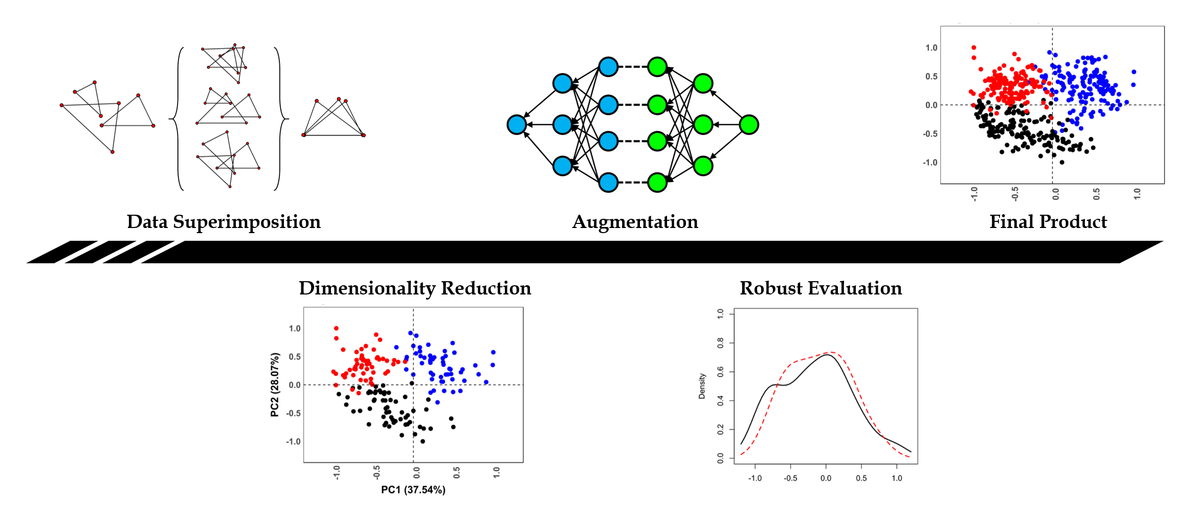
GM practices first project landmark configurations onto a common coordinate system. This process is carried out via a series of superimposition procedures, including scaling, rotation and translation, frequently known as Generalized Procrustes Analyses (GPA). GPA is a powerful technique that allows for the direct comparison of landmark configurations, quantifying minute displacements of individual landmarks in space [5,6]. These distortions and deformations can then be used to highlight geometric variations among organisms and can be visualized with ease.
From these superimposed configurations, matrix operations from linear algebra can be performed to project each element under study as a single multidimensional (ℝn) point in a newly constructed feature space. This procedure, known as Principal Components Analysis (PCA) is useful for dimensionality reduction and converting landmarks into more manageable data for complex statistical applications [7,8].
A wide array of techniques are known for different pattern recognition and classification tasks in GM. From one perspective, more traditional parametric and non-parametric multivariate statistical analyses can be performed to assess differences and similarities among sample distributions [7]. Likewise, generalized distances and group association probabilities can be used to compare groups of organisms and trends in variation and covariation [9]. Moreover, many popular classification tasks rely on parametric discriminant functions [10,11].
In more recent years, tasks in pattern recognition and classification have received an increase in efficiency and precision with the implementation of Artificially Intelligent Algorithms (AIAs), reporting >90% accuracy in GM applications. In a broad sense, AIAs are algorithms designed to “learn” from data so as to perform a wide array of different tasks. In this context, AIAs can be programmed to automatically learn from subsets of data to adjust their internal parameters, while using other subsets to validate these parameters for performing a certain task [12]. Among the multitude of available algorithms, the most popular AIAs for classification purposes in GM currently include Support Vector Machines (SVM) [13,14,15,16], and Artificial Neural Networks (ANN) [17,18,19,20,21]. Both algorithms present distinct advantages, especially in the processing of complex high-dimensional data. As opposed to traditional Linear and/or Partial Least-Squares Discriminant Analyses (LDA and PLSDA), SVMs and ANNs are less susceptible to underlying assumptions within model properties. SVMs, for example, are able to use numerous different kernel functions to overcome issues imposed by linearity [22,23]. ANNs, on the other hand, are highly versatile non-linear algorithms inspired by information processing in the brain, achieving above human performance in a multitude of real-life situations [23,24,25].
Nevertheless, each of these types of analyses are susceptible to a number of different problems, all of which can affect the reliability of the extracted data. From one perspective, numerous studies have focused on the error produced through data collection procedures, whether this type of error be induced by analyst experience, collection protocols or the definition of the landmark itself [26,27,28,29].
Landmarks, for example, can be divided into several different types. While some of the original definitions of landmark types were based on strictly biological features [30], these definitions can be considered somewhat restrictive for morphological analyses outside of anatomy. Under this premise, we prefer to define landmarks in a more general sense (Figure 1), referring to Type I landmarks as anatomical points of biological significance [3,30]; Type II landmarks can be defined as points of mathematical significance (e.g., maximal curvature or length) [3]; and Type III landmarks can be considered constructed points located around outlines or in relation to other landmarks [3]. From another perspective, valuable contributions in the field of GMs have seen the incorporation of computational landmarks into analyses. From this perspective “semi-landmarks” can be computed that “slide” over curves and surfaces in an attempt to reduce bending energy [4]. Finally other promising efforts have been made to develop automated tools for landmark digitization [31].
With both a more generalized definition of landmark types, as well as the inclusion of computational tools for their digitization, GMs have been able to quantify morphological traits across a wide array of different objects (Figure 1), including stone implements and tools [32], as well as microscopic anomalies found on bone [14,15,16,21,29].
More often than not, however, the preservation rate of fossils results in the loss of landmarks, impeding many types of analyses [33,34]. The completeness of the fossil record is thus a major conditioning factor in archaeological and paleontological GM analyses. Considering the number of available fossils for certain species, construction of reliable datasets is difficult, resulting in sample bias. Statistical tests such as Canonical Variant Analyses (CVA), for example, are highly sensitive to small or imbalanced datasets [9]. Moreover, the impact of bias is directly proportional to the number of variables included in multivariate analyses [35]. Even if samples are balanced, in fields such as paleoanthropology obtaining large sample sizes is often difficult, and thus the predictive capacity of discriminant models may fall significantly.
1.2. Data Augmentation
Resampling techniques in traditional statistics have had great success in providing more robust methods to test statistical approximations and p-value calculations. Tests requiring permutations as well as more computationally efficient Monte Carlo simulations have been a standard procedure in statistical practices for over half a century [36,37]. Their versatility to both parametric and non-parametric assumptions makes handling imbalanced and skewed data much more reliable, while proving less sensitive to samples of smaller sizes [38]. Nevertheless, a critical issue when considering small sample sizes are an “insufficiency of information density” that is able to correctly provide a general overview of the population’s distribution [39]. This issue becomes apparent when trying to classify new individuals. With insufficient knowledge of the true coverage of a domain, the interpretation of new information is much more difficult. In data science this phenomenon is usually known as overfitting for classification algorithms [25].
One statistical technique frequently used to overcome this issue is resampling with replacement, known as bootstrapping. Bootstrapping duplicates the data multiple times creating a virtual population from a distribution sample [40,41]. As opposed to resampling techniques without replacement (e.g., permutation, cross-validation, jackknife), bootstrap procedures are efficient in inferential tasks helping to simulate the general nature of the population. Nevertheless, neither of these resampling procedures, in truth, simulate new information. While they may be useful for inflating the dataset and providing enough information for a model to adjust its weights, overfitting is likely, as the space between data points can still be considered “uncharted territory”.
In response, data scientists and specialists in AIAs propose the use of synthetically produced new data to overcome these problems [42]. While using synthetic “fake” data has drawn some skepticism from scientists, numerous experiments in predictive modelling have empirically shown how these synthetic datasets not only reduce overfitting, but actually produce an increase in accuracy [43]. This is achieved through creating new data that is “meaningful” to the real distribution by adapting the data that is already available [44] (Tanaka and Aranha, 2019). These advances have had a major impact on scientific disciplines dedicated to computational learning, especially in the case of highly complex applications for computer vision [25]. One of the key AIAs responsible for this success is the Generative Adversarial Network (GAN).
GANs were originally presented as an unsupervised AIA capable of creating new data, based on the training data provided [45]. In less than a decade, GANs have been efficiently incorporated into a wide variety of applications, especially in fields of computer vision and image processing. A GAN consists of two neural networks trained simultaneously. The first model, known as the Generator, is trained to produce synthetic information which the second model, the Discriminator, evaluates for authenticity. The two models are trained in competition (i.e., adversarial), with the generator working to produce data that the discriminator is unable to classify as synthetic. The final product is a generator model capable of producing completely new data that is indistinguishable from the real training set. With the additional advantage of a neural network’s non-linear internal configuration, GANs are highly efficient in mapping out any type of probability distribution. From this perspective, GANs have been used for a wide arrange of different applications, including the generation of photo-realistic images, anomaly detection, music generation, and the approximation of a number of different statistical distributions [46,47].
2. Materials and Methods
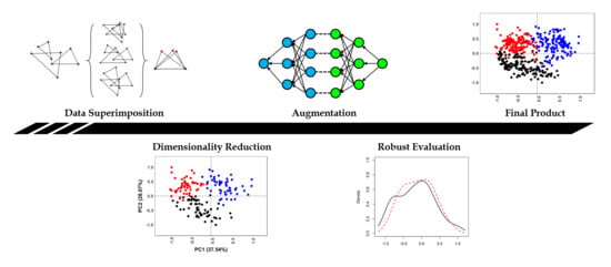
This study presents an experimental protocol used to evaluate and assess different types of GANs for augmenting GM datasets. Through experimenting with different architectures, configurations and training strategies, this study aims to propose an optimal architecture for augmenting data of this type. In order to evaluate these results, both descriptive statistics and equivalency testing have been used. Figure 2 presents a general visualization of the described workflow.
2.1. Datasets
Experiments included within this study were performed on a total of three GM datasets. These datasets originated from experimental archaeology samples in taphonomy. Each of these samples thus represent the morphological features of microscopic alterations observed on bone, using GM to quantify these morphologies for diagnostic purposes.
Nevertheless, considering the objective of this study is to observe the effects of generative learning for GM data augmentation, the origin of these datasets was considered unimportant. The reason behind this lies in how, regardless of the element under study, data used for GM analysis consists of superimposed landmark coordinates (Figure 1 and Figure 2). From these coordinates, dimensionality reduction can be used to convert each element into a single vector from which models can learn from (Figure 2). Therefore, irrespective of whether the raw landmark data was obtained from paleoanthropological specimens, lithic tools or carnivore feeding samples (Figure 1), all landmarks are similarly embedded into a single vector that can be used as the input to our computational models. Additional use of these three case studies was based on how each dataset was personally generated by the corresponding author, providing a means of controlling the origin of information.
The 3 datasets used consists of a mixture of manually placed landmarks (Type II or III; Figure 1), as well as some computational semi-landmarks [3,4]. The three datasets include;
- Dataset 1 (DS1); canid tooth score dataset [16]. This dataset consists of 105 individuals from three different experimental carnivore feeding samples (labelled foxes, dogs and wolves). 3D models for data extraction were generated using a low-cost structured light surface scanner (David SLS-2). The topography of each 3D digital model was then used to extract 2D images where landmarks could be placed. Landmark data consist of a mixture of Type II and Type III 2D landmarks.
- Dataset 2 (DS2); scratch and graze trampling dataset [15]. This dataset consists of 60 individuals from two different experimental trampling mark samples (labelled scratches and grazes). Each of the elements under study were digitized employing a 3D Digital Microscope (HIROX KH-8700), using between 100× and 200× magnification. Collection of landmark data was then performed following a series of measurements that established a 3D coordinate system across the model. Landmark data consist of a mixture of Type II and Type III 3D landmarks.
- Dataset 3 (DS3); semi-landmark based tooth pit dataset [29]. This dataset consists of an adaptation of DS1 using 60 individuals from two carnivore feeding samples (labelled dogs and wolves). 3D models for data extraction were generated using a low-cost structured light surface scanner (David SLS-2). Landmark data consist of a mixture of 3D Type II landmarks and a mesh of semi-landmarks.
These three datasets were chosen considering the dimensionality of the corresponding feature-space produced for GM analysis (ℝ14, ℝ39 and ℝ60 respectively). With each of these datasets presenting different dimensionalities, optimal GAN architectures could therefore be proposed so as to establish a standardized protocol, regardless of the target domain’s ℝn size.
These datasets were also chosen to observe the effect original sample size has on the accuracy of synthetic data. The latter was tested via minimum sample size calculations according to Cohen’s d (power = 0.8, d = 0.8, α = 0.05, ratio = 1:1) [35]. This established a minimum sample size for two-sample statistical comparisons of 26 individuals, rounded up to 30 for simplicity. In accordance with this calculation, experiments were performed by randomly sampling 30 real individuals and comparing them with 30 synthetic individuals. In datasets where larger samples were available, 60 real individuals were sampled and compared with 60 synthetic data points.
2.2. Baseline Geometric Morphometric Data Acquisition
Each of the datasets were prepared using traditional GM techniques, first performing a full Procrustes fit of landmark coordinates via GPA (Figure 2), followed by the extraction of multivariate features through PCA [7,8]. Considering how the objectives of this study are to find the optimal algorithm for mapping out multidimensional distributions, differences in shape-size relationships were considered irrelevant for this study. GPA was therefore only performed using fully superimposed coordinates in shape feature space.
From here, PC scores were analyzed evaluating their dimensionality and the proportion of variance represented across each of the decomposed eigenvectors and their eigenvalues. Considering how the final eigenvalues begin to represent little or no variance within the landmark configuration, preference was given to those PC scores representing up to 95% of sample variance for statistical evaluations.
For the purpose of this study, GM pre-processing of samples was performed in the free statistical software R (https://www.r-project.org/, v.3.5.1 64-bit).
2.3. Generative Adversarial Networks
A GAN is a Deep Learning (DL) architecture used for the synthesis of data via a generator model. GANs are fit to data using an unsupervised approach, where the generator is trained by competing with a discriminator that evaluates the authenticity of the synthetic data produced [24,41]. While the basic concept behind a GAN is relatively straightforward, the theory behind their configuration and training can be incredibly challenging [25,48,49,50,51].
To generate new data, the generator samples from a random Gaussian distribution (e.g., µ = 0, σ = 1), finding the best means of mapping this data out onto the real sample domain. A fixed-length random vector is used as input, triggering the generative process. Once trained, this vector space can essentially be considered a compressed representation of the real data’s distribution. This multidimensional vector space is most commonly referred to in DL literature as latent space [21,48].
The discriminator model takes as input the output of the generator. This discriminator can then be used to predict a class label (real or fake) for the generated data. In some cases, this model is referred to as a critic model [52,53].
For the purpose of this study, multiple experiments were performed to define an optimal GAN architecture. These experiments followed standard DL protocol, finding the optimal neural network configurations by evaluating the effects of each hyperparameter on model performance. Summaries of the hyperparameters tested are included in Table 1.
In addition to this, the extensive literature on the “best-practices” in GAN research and different heuristics in GAN hyperparameter selection were considered [48,49,51,54]. Among these, common “GAN-Hacks” were evaluated, including:
- Use of the Adam optimization algorithm (α = 0.0002, β1 = 0.5)
- Use of dropout in the generator with a probability threshold of 0.3
- Use of Leaky ReLU (slope = 0.2)
- Stack hidden layers with increasing size in the generator and decreasing size in the discriminator.
For training, trials experimenting with the number of epochs and batch sizes were performed. The final values were chosen in accordance with the requirements of the model in order to reach an acceptable stability.
While binary cross-entropy is typically a recommended loss function for training, this study experimented with alternatives, such as the Least Squares loss function (LSGAN) and two versions of Wasserstein loss (WGAN). LSGAN was originally proposed as a means of overcoming small or vanishing gradients, which are frequently observed when using binary cross-entropy [50,52]. In LSGAN, the discriminator (D) attempts to minimize the loss (L), using the sum squared difference between the predicted and expected values for real and fake data (Equation (1)), while the generator (G) attempts to minimize this difference assuming data is real (Equation (2)):
This results in a greater penalization of larger errors (E) which forces the model to update weights more frequently, therefore avoiding vanishing gradients [55]. WGAN, on the other hand, is based on the theory of Earth-Mover’s distance [52], calculating the distance between the two probability distributions so that one distribution can be converted into another (Equations (3) and (4)):
WGAN additionally uses weight constraints (hypercube of [−0.01, 0.01]) to ensure that the discriminator lies within a 1-Lipschitz function. In certain cases, however, this has been reported to produce some undesired effects [53]. As an alternative, a proposed adaptation, in the form of gradient penalty WGAN (WGAN-GP), includes the same loss for the generator (Equation (4)) but a modified discriminator (eg., 5) with no weight constraints [53,56]:
For both loss functions to work, the output of D requires a linear activation function. Finally, optimization tests were performed using Adam (α = 0.0002, β1 = 0.5) and RMSprop (α = 0.00005) [50,53,57,58].
More details on the mathematical components of each GAN loss function can be consulted in the corresponding references [25,50,52,53,55].
GANs were trained on scaled PCA feature spaces with 64-bit values ranging between 1 and −1. This scaling procedure was performed to boost neural network performance and optimization by helping reduce the size of weight updates [24]. For these experiments, GANs were trained on all data within the dataset, regardless of label. This approach was chosen to directly observe how GANs handle this type of input data before considering more complex applications, including sample labels. (See Section 2.4)
All experiments were performed in the Python programming language (https://www.python.org/, v.3.7 64-bit) using TensorFlow (https://www.tensorflow.org/, v.2.0). Neural networks were compiled and trained on the CPU of an ASUS X550VX laptop (Intel® CoreTM i5 6300HQ).
2.4. Conditional Generative Adversarial Networks
The final GAN trials performed adapted the optimally defined model in Section 3.1 for Conditional GAN tasks (CGAN). A CGAN is an extension of traditional GANs that incorporate class labels into the input, thus conditioning the generation process. Class labels are encoded and used as input alongside both the latent vector and the original vector in order for the GAN to learn targeted distributions within the dataset [59]. This can be done by using an embedding layer and concatenating the embedded information with the original input [60]. It is recommended that the embedding layer is kept as small as possible [51], with some of the original implementations of CGANs using an embedding layer with a size of only ≈5% of the original flattened generator’s output. Because 5% of our largest dataset would still have been <1, experiments were performed with different sized embedding layers to find the optimal configuration. The best results came out using a ⌈1/4 • n⌉ sized embedding layer, where n corresponds to the number of dimensions in ℝn for each of the targeted feature spaces.
For comparison of GAN and CGAN performance, these models were used separately to augment the DS3. This dataset was chosen considering it was the most complex feature space to map, the most balanced (when compared with DS1), and the most difficult to study (seeing how DS2 presents the highest natural separability).
2.5. Synthetic Data Evaluation
Evaluation of GANs is a complex issue with little general agreement on suitable evaluation metrics [49]. Considering how most practitioners in GAN research work with computer vision applications, many papers use manual inspection of images to evaluate synthesized data [61]. Image evaluation, for example, often consists in the visualization of GAN outputs to check whether they are realistic or not, or the use of specified algorithms that are very image-specific [61]. For the synthesis of numeric data, manual inspection is evidently a very subjective means of evaluating information, while calculations such as Inception-score are not applicable to this type of data [49,61,62]. Under this premise, the majority of metrics used in GAN literature is of little value to the present study, as they almost exclusively focus on the evaluation of images [60,62].
Multidimensional numbers are incredibly difficult to visualize, meaning that precise human inspection of this data is impossible. To overcome this, a number of statistical metrics were adopted for GAN evaluation.
Firstly homogeneity of GM data was tested. In most traditional cases, the elimination of size and preservation of allometry in GPA is known to normalize data [63]. Nevertheless, this assumption does not always hold true. The first logical step was to therefore evaluate distribution homogeneity and normality via multiple Shapiro tests. Synthetic distributions were then compared with the real data to assess the magnitude of differences and the significance of overlapping. For this, a “Two One-Sided” equivalency Test (TOST) was performed. TOST evaluates the magnitude of similarities between samples by using upper (εS) and lower (εI) equivalence bounds that can be established via Cohen’s d. This assesses H0 and Ha using an α threshold of p < 0.05, with Ha implicating significant similarities among samples [35,64,65,66,67]. For TOST the test statistics used to assess these similarities were dependent on distribution normality. These varied between the traditional parametric method using Welch’s t-statistic [68], or a trimmed non-parametric approach using Yuen’s robust t-statistic [69,70]. To differentiate between the two, from this point onwards non-parametric robust TOST will be referred to as rTOST.
More traditional univariate descriptive statistics were also employed. For distributions matching Gaussian properties, sample means and standard deviations were calculated. These were accompanied by calculations of sample skewness and kurtosis. For significantly non-Gaussian distributions, robust statistical metrics were used instead. In these cases, measurements of central tendency were established using the sample median (m), while deviations were calculated using the square root of the Biweight Midvariance (BWMV) (Equations (6)–(9)) [29,71,72].
Robust skewness and kurtosis values were calculated using trimmed distributions. Trims were established using Interquatile Ranges (IR) [71], with confidence intervals of p = [0.05:0.95]. Both the IR range and the trimmed skewness and kurtosis values were reported.
Finally, wherever possible, correlations were calculated to compare the effect of hyperparameters on the quality of synthesized data. For homogeneous data, the parametric Pearson test was used [73], whereas inhomogeneous data was tested using the non-parametric Kendall τ rank-based test [74]. Considering neural networks are stochastic in nature, these correlations were performed using data obtained from multiple training runs of each GAN to ensure a more robust calculation.
3. Results
All three datasets analyzed present highly inhomogeneous multivariate distributions (p < 2.2 × 10⁻¹⁶). Univariate comparisons (Table 2), however, present a mixture of both inhomogeneous and homogeneous distributions across PC1 and PC2, where the majority of variance is represented.
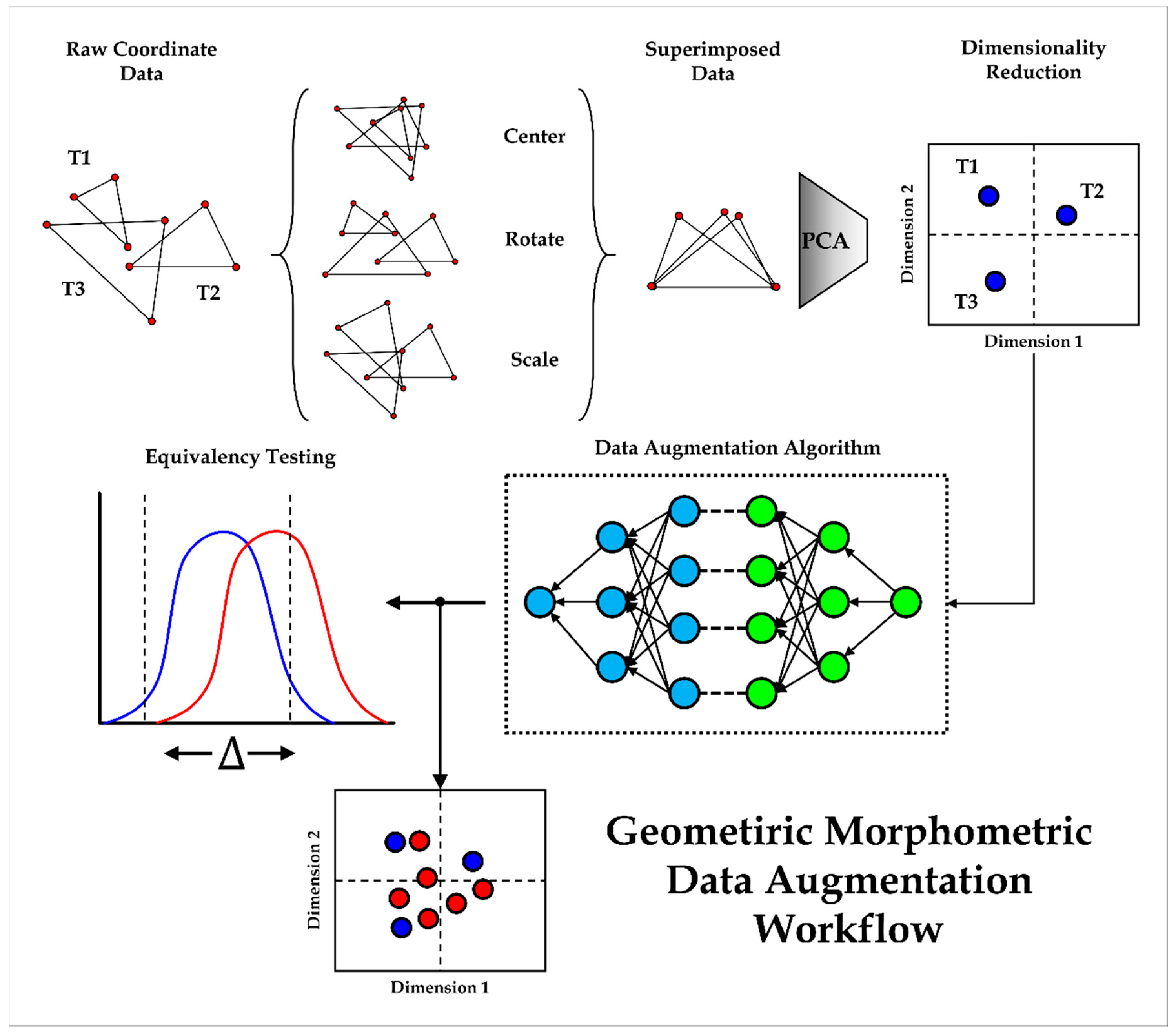
GAN failure through mode collapse was frequently observed throughout most of the initial trials, characterized by an intense clustering of points with little to no variation in feature space (Figure 3). Qualitatively, this type of failure is easily diagnosed by visual inspection of graphs. Quantitatively, mode failure can be characterized by a dramatic decrease in variance seen through deviation metrics. To provide an example, Figure 1 presents the use of a vanilla GAN trained on DS2. At first, training can be seen to start well with the closest (yet not optimal) approximation to the target domain’s median (Figure 3A). Nevertheless, little variation is present (BWMV of PC1 = 0.14, target BWMV = 0.38). As training continues, the algorithm is unable to find the correct median, and performance is seen to deteriorate (Figure 3B). This presents an exponential decrease in the variance of synthetic data (Figure 3B PC1 BWMV = 0.02, Figure 3C PC1 BWMV = 0.0002). Likewise, through mode collapse, the generator is unable to map the true normality of the distribution, generating increasingly normal data in PC1 (Shapiro w > 0.98, p > 0.56).
Replacing Leaky ReLU with tanh activation functions resulted in a significant improvement of generated sample medians (difference in median for Leaky ReLU = 0.78; tanh = 0.26), yet with little improvement in BWMV.
To overcome mode collapse, kernel initializers and batch normalization algorithms were incorporated into both the generator and the discriminator. Batch normalization was included before activation, presenting an increase in BWMV. Initializers required careful adjustment, with small standard deviation values resulting in mode collapse. Additional experiments found the discriminator to require a more intense initializer (σ = 0.1) than the generator (σ = 0.7), while optimal results were obtained using a random normal distribution. Such a configuration allows the generator more room to adjust its weights, finding the best way of reaching the target domain’s median and absolute deviation while preventing the discriminator from learning too quickly.
Experiments adjusting hidden layer densities found symmetry between the generator and the discriminator to be unnecessary. The generator was seen to require more hidden layers in order to learn the distributions efficiently, while a larger density than the output in the last hidden layer also produced an increase in performance. The discriminator worked best with just two hidden layers.
3.1. Optimal Architectures
To optimally adjust these finds with all three datasets, the best GAN architecture that presented no mode collapse was obtained using 3 hidden layers in the generator and two hidden layers in the discriminator. The size of hidden layers are conditioned by the size of the target feature space (Figure 4). To use the example of the largest target domain (DS3 = ℝ60), the generator is programmed so that the first hidden layer (Gh1) is a quarter of the size of the target vector (in this case Gh1 = 60·1/4= 15). If this calculation produces a decimal value (e.g., 59/4 = 14.75), the ceiling of this number is taken (⌈1/4·59⌉ = 15). This is followed by a layer half the size of the target vector (Gh2 = ⌈1/2·60⌉ = 30). The generator’s final hidden layer is the size of the vector plus one quarter (Gh3 = ⌈1/4·60⌉ + 60 = 75). The discriminator, on the other hand, is composed of two hidden layers, with the first hidden layer being the same size as Gh2, and the second hidden layer equivalent to Gh1. Each hidden layer is followed by a batch normalization algorithm before being activated using the tanh function. Tanh works best considering the target domain is scaled to values between -1 and 1. Other components of the algorithm include a dropout layer (p = 0.4) prior to the discriminator’s output and random normal kernel initializers in both models (discriminator σ = 0.1, generator σ = 0.7).
Experiments with loss functions and optimization algorithms showed a significant improvement in performance using LSGAN and WGAN variants when compared with vanilla GAN’s binary cross-entropy (rTOST p < 0.05, Table 3 with more details explained in Section 3.2). All three GANs were able to generate realistic distributions, with WGAN-GP outperforming WGAN in some cases (Table 3). LSGAN additionally worked best when using Adam optimization (α = 0.0002, β1 = 0.5), while WGAN and WGAN-GP excelled using RMSprop (α = 0.00005).
The optimal batch number was found at 16. This allowed the discriminator enough data to objectively evaluate performance and, thus, resulted in more efficient weight updates for the generator. The number of epochs, however, were highly dependent on the number of individuals used for training. Finally, the dimensionality of latent space was also found to be conditioned by the size of the target domain, as will be explained in continuation.
3.2. Experiments with Dimensionality and Sample Size
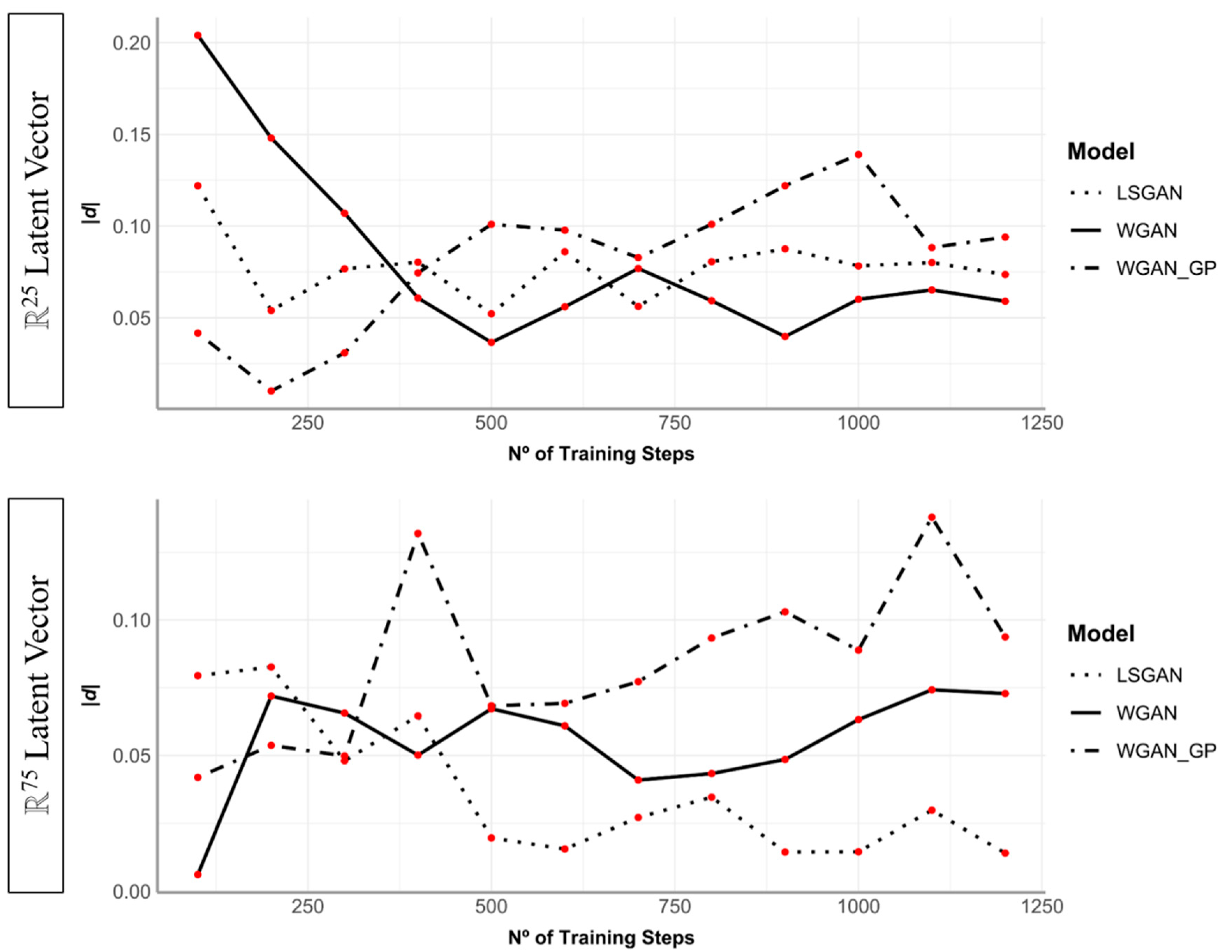
Initial trials with latent space found ℝ50 to produce the best results on average, especially in the case of DS2 (results of which have already been reported in Table 2). Nevertheless, interesting patterns emerged when experimenting with larger and smaller latent vector inputs. Starting with the case of the smallest target domain (DS1, Table 4), a significant negative correlation was detected when observing rTOST p values compared with the size of the latent vector over numerous runs (Kendall’s τ = −0.44, p = 0.001). This is also true when considering rTOST absolute difference values (τ = −0.41, p = 0.003). This correlation highlights larger ℝns to work best when working with smaller target domains. When training on larger feature spaces (e.g., DS3, Table 5), correlations proved insignificant for both rTOST p values (Kendall’s τ = −0.21, p = 0.13) and absolute difference calculations (τ = −0.29, p = 0.15). Nevertheless, while correlations remain insignificant, smaller latent vectors were seen to create more predictable and stable data (Figure 5).
In most experiments, 400 epochs were considered enough for GANs to produce realistic data. Moreover, the best results of each GAN began appearing after approximately 100-130 epochs. Performance significantly decreased, however, when trained on the same number of epochs using less data. To test this, subsets of each dataset were taken for experimentation (e.g., 30 out of 60 samples from DS2, Table 6). On all accounts, significant correlations were detected, finding smaller datasets to need more training time in order to obtain optimal results (Pearson’s r = 0.65, p = 0.0005). Likewise, LSGAN appeared to be the model least affected by dataset size, producing the most realistic distributions in each of the cases (Table 6). While training GANs using 400 epochs is still able to produce realistic data on small datasets, when considering the optimal number of epochs, increasing this number to 1000 produces a significant improvement in results.
3.3. Data Augmentation Results
3.3.1. General GAN Performance
All three GANs are highly successful in replicating sample distributions, effectively augmenting each of the distributions without too much distortion (Figure 7, Tables S1–S6). While evaluating standalone synthetic data creates some confusion, seen in some deviations of synthetic central tendency values and IR intervals (Tables S1, S3 and S5), the true value of GANs are observed when considering the augmented sample as a whole (Tables S2, S4 and S6).
In most cases, it can be seen how even the worst performing algorithms are able to maintain the central tendency of samples while boosting the variance represented. It is also important to highlight that, while in some cases central tendency can be seen to deviate slightly from the original distribution (e.g., LSGAN on DS2, Table S2), this is normally only true of one PC score and is still insignificant (rTOST p < 0.05). Some algorithms are also seen to affect the normality of sample distributions, creating distortion that is reflected in increased sample skewness. Nevertheless, these distortions are still unable to modify the general magnitude of similarities between synthetic and real data.
The greatest value of GANs can, therefore, be seen in increases in overall sample variance without significant distortion of the real sample’s distribution. Deviation values and IR intervals increase, representing more variability without significantly shifting central tendency and without generating outliers. This shows how each algorithm is able to essentially “fill in the gaps” for each distribution while staying true to the original domain.
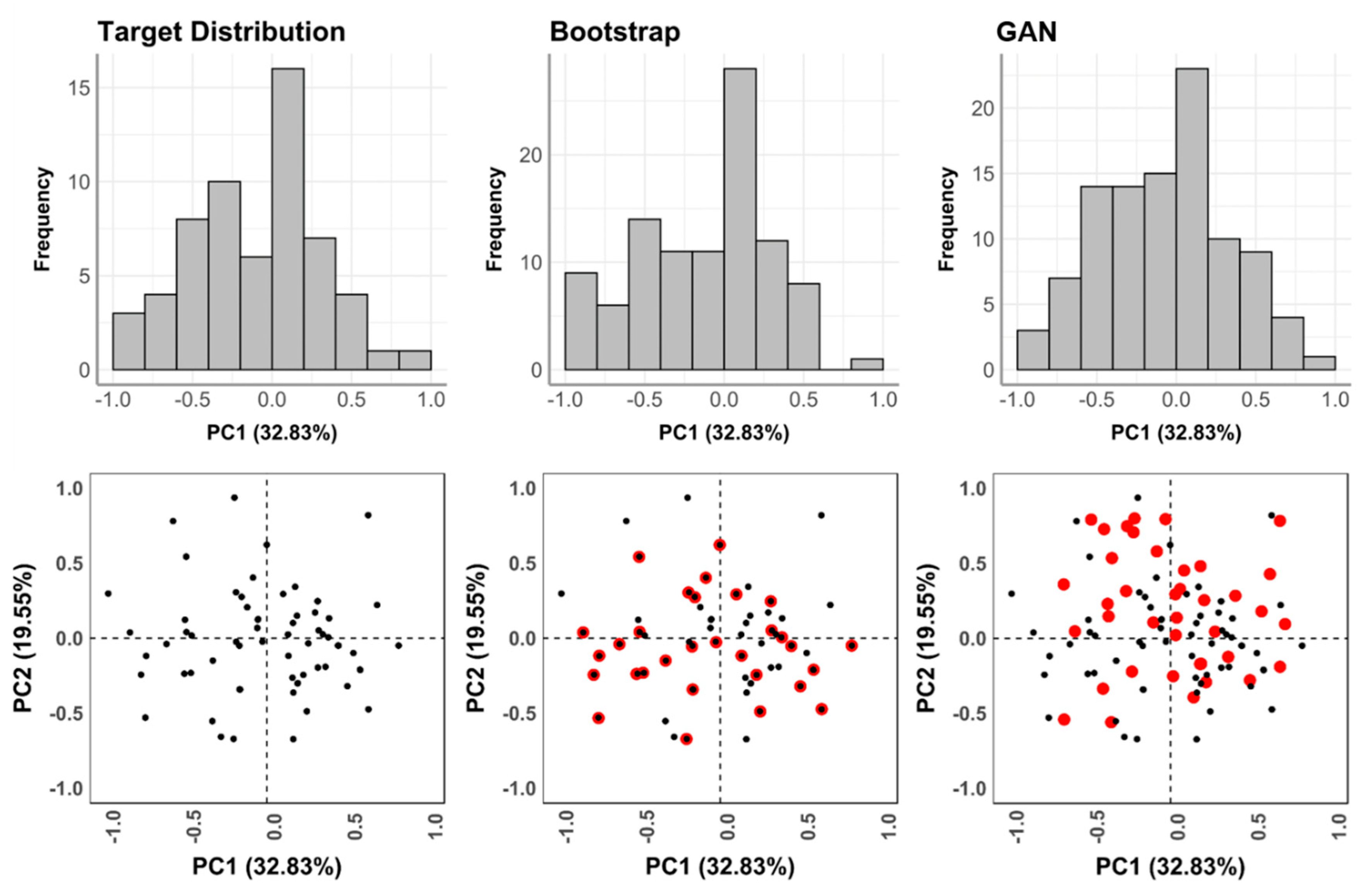
If GAN performance were to be compared with more traditional augmentation procedures, such as bootstrap, GANs can be seen to smooth out the distribution curve (Figure 8), creating a more general and complete mapping of the target domain. Bootstrapping procedures, on the other hand, tend to exaggerate gaps in the distribution. This can mostly be characterized by noticeable modifications to sample kurtosis while maintaining the general variation (Table 7).
3.3.2. Conditional GAN Performance
CGAN presented limited success when augmenting datasets, with only Wasserstein Gradient Penalty loss succeeding in overcoming mode collapse. Nevertheless, CGAN was still able to generate data with insignificant differences (Table 8), successfully augmenting the targeted datasets (Table 9 and Figure 9).
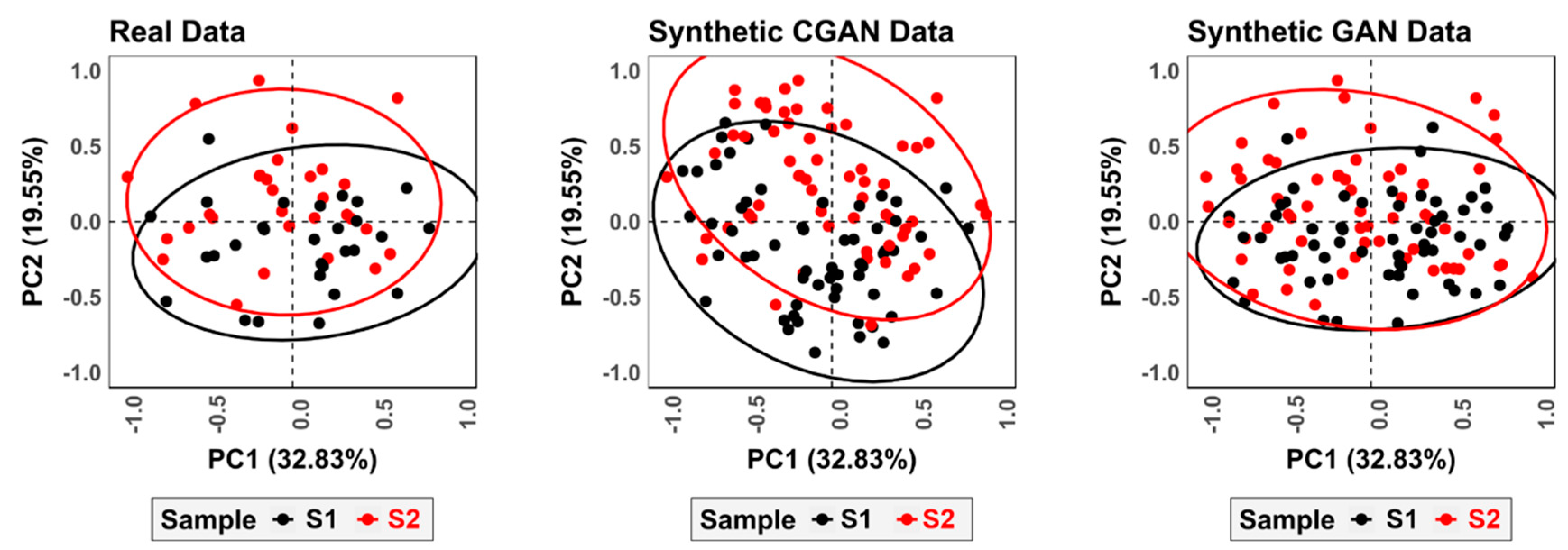
When taking a closer look at the performance of CGAN, however, it is important to note that, while the magnitude of differences between synthetic and real data are insignificant, CGAN distorts the original distribution to a greater degree (Figure 9). In both samples, CGAN deviates greatly from the target central tendency (Table 9) and appears to shift the general skew of the distribution (Figure 9). When using GANs to augment each of the samples separately, however, the generated data is arguably truer to the original domain. This is not to say, however, that CGANs are unable to augment feature spaces successfully. With the right configuration, CGANs are likely to reach similar results to traditional GANs. This, however, goes beyond the scope of the present study.
4. Discussion
Many algorithms require large amounts of data in order to efficiently extract information, a task which is particularly difficult when considering data derived from the fossil record. To confront this topic, this study presents a new integration of AIAs into archaeological and paleontological sciences. Here GANs have been shown to be a new and valuable tool for the modelling and augmentation of GM data. Moreover, these algorithms can additionally be employed on a number of different types of datasets and applications; whether this be the handling of paleoanthropological, biological, taphonomic or lithic specimens via GM landmark data.
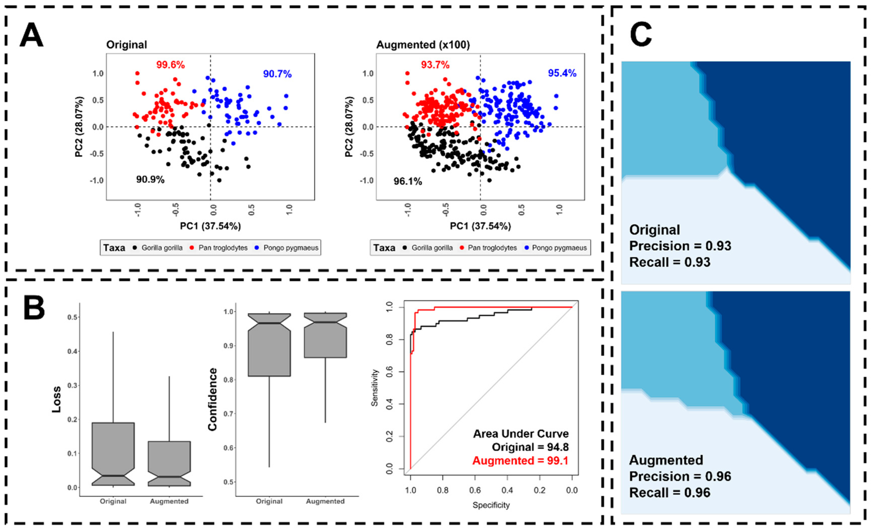
To demonstrate this latter point, and applying typical geometric morphometric techniques for classification on the O’Higgins and Dryden [75] Hominoid skull dataset, the present study is able to increment balanced accuracy of traditional LDA up to ca. 5% (Figure 10a) with a significant increase in generalization (Figure 10b,c). For this demonstration LDA was trained using a traditional approach [11], as well as an augmented approach based on Machine Teaching [43]. It can be seen how applying Machine Teaching using 100 realistic synthetic points per sample for training, and the original data was used for testing, helps the generalization process (Figure 10b) while providing clearer boundaries for each of the sample domains (Figure 10c).
It is important to point out, however, that this is not the solution to all sample-size related issues, and a number of components have to be discussed before more advanced applications can be carried out.
Missing data and the availability of fossil finds are a major handicap in prehistoric research. This is increasingly relevant when considering fossils of older ages, such as individuals of the Australopithecus, Paranthropus and early Homo genera. In a number of cases, for example, the representation of Australopithecine or Homo erectus/ergaster specimens may not even surpass 10 individuals [76,77,78], while Homo sapiens specimens are in abundance. In these cases, and in accordance with the data presented here, GANs would not be able to successfully augment the targeted minority distributions from scratch. Other options, however, could entail the use of algorithms for pre-processing, using variations of the Synthetic Minority Oversampling Technique (SMOTE & Borderline-SMOTE) [79,80,81], or the adapted version Adaptive Synthetic Sampling (ADASYN) [82].
Both SMOTE and ADASYN are useful, easy to implement algorithms that augment minority samples in imbalanced datasets. SMOTE generates synthetic data in the feature spaces that join data points (e.g., according to k nearest-neighbor theory), thus filling in regions of the target domain [79,80,81]. ADASYN takes this a step further by modelling on sample distributions based on data-density [82]. Both are valuable algorithms that have become popular in imbalanced learning tasks, generally improving predictive model generalization. Nevertheless, their application should be confronted conservatively.
Preliminary experiments within this study found that resampling via bootstrapping prior to the training of GANs resulted in severe mode collapse. This can be theoretically explained by the manner in which bootstrapping is over-inflating the domain and highlighting very specific regions which the model then learns from. This results in overfitting as the model is repeatedly learning to map out the same value multiple times, boosting the probability of mode collapse through an enhanced lack of variation in the original trainset. Considering how SMOTE and ADASYN produce more “meaningful” data [44,79], these algorithms are more likely to aid the training process rather than produce the adverse effect. Nevertheless, overuse of SMOTE/ADASYN is likely to have a similar effect to bootstrapping, where linear regions of feature space between data points are enhanced while other regions are left empty.
Through this, the current study proposes that a conservative use of SMOTE or ADASYN variants prior to the training of GANs may be able to boost performance on overly-scarce datasets (e.g., the cases of [76,77,78]). This practice would be able to augment minority samples to a suitable threshold (n = 30), preparing the dataset for more complex generative modelling and enabling an improved generalization of any predictive models used in analyses that follow.
From a similar perspective, the use of Bayesian Inference Algorithms such as Markov Chain Monte Carlo (MCMC) and Metropolis-Hastings algorithms have also been known to effectively model from multiple types of probability distributions [83,84,85]. In some cases, it may be possible to use these approaches to sample from the probability distribution at hand, and produce simulated information from the target distribution which would essentially be more realistic than simple bootstrap approaches. Further research into how these approaches may be applied could provide a powerful insight into GAN alternatives for different types of numerical data in GM.
In the general context of computational modelling, common criticism of neural network applications in archaeology and paleoanthropology argue that GM datasets are generally insufficient for the training of AIAs. This is based on the fact that most DL algorithms require much more data to avoid overfitting. From this point of view, why would training a GAN on such little data be any different? The present study proves that this is not an issue, considering how, with only 30 individuals, GANs are still able to produce highly realistic synthetic data (LSGAN rTOST p = 3.8 × 10⁻²²).
In common DL literature, state-of-the-art models are reported to obtain ≈80% accuracy when trained on thousands to millions of specimens [25]. It is important to consider, however, that in the majority of these cases AIAs are trained on images (i.e., computer vision applications). To provide an example, Karras et al. [54] present a GAN capable of producing hyper-realistic fake images of people’s faces, building from a subset of the CelebA-HQ dataset using ≈30,000 images. Two main components must be considered in order to understand why such a large dataset is required for their model;
- Karras et al. [54] present a GAN capable of producing high resolution 1024x1024 pixel RGB images. In computer vision applications, each image is conceptualized as a multidimensional numeric matrix (i.e., a tensor). Each of the numbers within the tensor can essentially be considered a variable, resulting in a dataset of approx. three million variables per individual photo.
- In order to efficiently map out these three million numeric values, the featured GAN uses progressively growing convolutional layers (nº layers ≈ 60) with 23.1 million adjustable parameters.
- The present study uses feature spaces that have already undergone dimensionality reduction derived from GM landmark data. In the case of the largest dataset, this results in a target vector of 60 variables that need to be generated. The present study additionally only uses fully connected layers with no convolutional filters, resulting in a model of <11,000 adjustable parameters. A GAN targeting three million values with 23.1 million parameters would thus require a far larger dataset than one targeting 60 values with 11 thousand parameters, explaining why with just 30 specimens, GAN convergence is still possible.
Regardless of the mathematics behind DL theory, the statistical results presented here provide enough empirical evidence to argue the value of the proposed GAN with as little as 30 individuals. Nevertheless, even in cases where datasets are too scarce for GANs to be developed from scratch, pre-trained models can be adjusted to different domains via multiple DL techniques. This arguably opens up new possibilities for the incorporation of Transfer Learning into GMs [25].
Finally, it is important to highlight how no absolute protocol can be established for generative modelling of any type. DL practitioners are usually required to adapt their model according to the dataset at hand, using the best practices established in other studies as a baseline from which to work from. Under this premise, recommendations established for the augmentation of GM datasets using GANs can be listed as follows:
- Best results are obtained when scaling the target domain to values between −1 and 1.
- Hidden layer densities should be adjusted according to the number of dimensions within the target domain (Figure 4). Tanh activation functions in both the generator and the discriminator are recommended.
- Dropout, batch normalization and kernel initializers (discriminator σ = 0.1, generator σ = 0.7) are recommended to regulate the learning process and avoid mode collapse.
- The Adam optimization algorithm is recommended when using Least-Square loss, while RMSProp is more efficient when using the Wasserstein (WGAN or WGAN-GP) function. A minimum batch size of 16 obtains the best results.
- LSGAN is recommended when training data is limited, increasing the number of epochs to at least 1000.
- WGAN and WGAN-GP work best on larger datasets, while approximately 400 epochs are usually enough to produce realistic data.
- The smaller the target domain, the larger the latent vector required for generator input.
- For conditional augmentation, optimal results are obtained by training GANs on each sample separately, rather than using CGANs.
5. Prospective and Future Research
While GANs are difficult to develop, the complexity of these AIAs should not be cause for discouragement. There currently exists a wide range of literature and helpful guides dedicated to teaching scientists about AIA development, even for those with no background in mathematics or applied statistics. With platforms such as ScienceDirect (https://0-www-sciencedirect-com.brum.beds.ac.uk/) in 2019 alone reporting over 3000 papers including the term Deep Learning (in keywords, title or abstract), and ca. 6000 for Machine Learning, AI can be considered one of the most popular lines of research in modern science. This presents a promising future for applications in archaeological and paleontological research.
Future lines will thus address the testing of GAN performance in actual archaeological and paleontological studies. Likewise, it would be highly recommendable to test whether these algorithms can effectively model data of a non-GM origin, employing the robust statistical techniques described here for more empirical evaluations of numeric data. Finally, comparisons with other augmentation techniques could help provide a more global view of the tools available for researchers.
6. Conclusions
To the authors’ knowledge, this is the first comparative study in DL and GM using GANs for high dimensional numeric simulations that further employ advanced descriptive statistical metrics for evaluation. While augmented data is by no means a substitute for real data, real-life DL practices and applications have shown “meaningful” synthetic data to significantly increase the confidence and power of statistical models. In many cases, this has even been seen to exceed human-level precision.
The present paper has shown how GANs can be trained efficiently on numerical data obtained using geometric morphometrics. Under this premise, whether geometric morphometrics be used for the analysis of biological or non-biological individuals, GANs can effectively be used for data augmentation techniques prior to any consequent statistical modelling or learning tasks. The present study has additionally shown that three different loss functions are able to effectively learn from this type of data. Finally, robust statistical metrics have proven a valuable tool for performance evaluation.
Supplementary Materials
The following are available online at https://0-www-mdpi-com.brum.beds.ac.uk/2076-3417/10/24/9133/s1, Table S1: Descriptive statistics for DS1 of both target and synthetic sample distributions when compared separately. Table S2: Descriptive statistics for augmented DS1. Table S3: Descriptive statistics for DS2 of both target and synthetic sample distributions when compared separately. Table S4: Descriptive statistics for augmented DS2. Table S5: Descriptive statistics for DS3 of both target and synthetic sample distributions when compared separately. Table S6: Descriptive statistics for augmented DS3.
Author Contributions
Conceptualization, L.A.C.; methodology, L.A.C.; software, L.A.C.; validation, L.A.C. and D.G.-A.; formal analysis, L.A.C.; investigation, L.A.C.; resources, L.A.C.; data curation, L.A.C.; writing—original draft preparation, L.A.C.; writing—review and editing, L.A.C. and D.G.-A.; visualization, L.A.C.; supervision, D.G.-A.; project administration, D.G.-A.; funding acquisition, D.G.-A. All authors have read and agreed to the published version of the manuscript.
Funding
L.A.C. is funded by the Spanish Ministry of Science, Innovation and Universities with an FPI Predoctoral Grant (Ref. PRE2019-089411) associated to project RTI2018-099850-B-I00 and the University of Salamanca.
Acknowledgments
The corresponding author sincerely appreciates the support and advice of his directors; José Yravedra, Rosa Huguet and D.G.-A. We are also grateful to Jason Brownlee for his excellent work on Artificial Intelligence and his useful advice over multiple email conversations. The present paper was written during the national Spanish lockdown for the COVID-19 pandemic (March–June 2020). With this in mind we would like to thank all those who contributed towards protecting our health and safety in and outside of the health, pharmaceutical and civil sectors. L.A.C. would also like to thank Noé Valtierra, Guillermo (Máster) Blanco, Zaira López-Arias, Miguel Ángel Moreno-Ibañez, Enrique de Casimiro, Juan Hernandez-Rubio, Sara García-Motilla and his family for their support. We also thank Jordan Courtenay for her help proofreading earlier versions of this paper. Finally we thank two anonymous reviewers and the editorial staff of MDPI for their useful comments and suggestions to improve the quality of our paper.
Conflicts of Interest
The authors declare no conflict of interest.
Data Availability
All data used in the current study has been fully sited and is available across multiple different data repositories. DS1 is available via a FigShare data repository (doi:10.6084/m9.figshare.c.4494218.v1). DS2 is included within supplementary files 1 and 3 of the associated paper [14]. DS3 is included within the corresponding author’s GitHub page within the folder titled Landmark_Files of the https://github.com/LACourtenay/GMM_Measurement_Accuracy_Tools repository. The O’Higgins and Dryden [69] dataset is included within the R “shapes” package and can be called via the command data(apes).
Code Availability
All python code for GAN and CGAN applications are available via the author’s GitHub page: https://github.com/LACourtenay/GMM_Generative_Adversarial_Networks.
References
- Bookstein, F.L. Morphometric Tools for Landmark Data; Cambridge University Press: Cambridge, UK, 1991. [Google Scholar]
- Bookstein, F.L. Landmark methods for forms without landmarks: Morphometrics of group differences in outline shape. Med. Image. Anal. 1996, 1, 225–243. [Google Scholar] [CrossRef]
- Dryden, I.L.; Mardia, K.V. Statistical Shape Analysis; John Wiley and Sons: New York, NY, USA, 1998. [Google Scholar]
- Gunz, P.; Mitteroecker, P.; Bookstein, F.L. Semilandmarks in three dimensions. In Modern Morphometrics in Physical Antrhopology; Slice, D.E., Ed.; Plenum Publishers: New York, NY, USA, 2005; pp. 73–98. [Google Scholar]
- Bookstein, F.L. Principal warps: Thin plate spline and the decomposition of deformations. IEEE Trans. Pattern Anal. Mach. Intel. 1989, 11, 567–585. [Google Scholar] [CrossRef] [Green Version]
- Ricthsmeier, J.T.; Lele, S.R.; Cole, T.M. Landmark morphometrics and the analysis of variation. In Variation; Hallgrimsson, B., Hall, B.K., Eds.; Elsevier Academic Press: Boston, MA, USA, 2005; pp. 49–68. [Google Scholar]
- Rohlf, F.J. Statistical power comparisons among alternative morphometric methods. Am. J. Phys. Antrhopol. 2000, 111, 463–478. [Google Scholar] [CrossRef]
- Klingenberg, C.P.; Monteiro, L.R. Distances and directions in multidimensional shape spaces: Implications for morphometric applications. Soc. Syst. Biol. 2005, 54, 678–688. [Google Scholar] [CrossRef] [PubMed] [Green Version]
- Albrecht, G.H. Assessing the affinities of fossils using canonical variates and generalized distances. J. Hum. Evol. 1992, 7, 49–69. [Google Scholar] [CrossRef]
- Barker, M.; Rayens, W. Partial least squares for discrimination. J. Chemom. 2003, 17, 166–173. [Google Scholar] [CrossRef]
- Mitteroecker, P.; Bookstein, F. Linear discrimination, ordination, and the visualization of selection gradients in modern morphometrics. Evol. Biol. 2011, 38, 100–114. [Google Scholar] [CrossRef]
- Bocxlaer, B.V.; Schultheiß, R. Comparison of morphometric techniques for shapes with few homologous landmarks based on machine learning approaches to biological discrimination. Paleobiology 2010, 36, 497–515. [Google Scholar] [CrossRef]
- Géron, A. Hands-on Machine Learning with Scikit-Learn, Keras & Tensorflow; O’Reilly: Tokyo, Japan, 2019. [Google Scholar]
- Courtenay, L.A.; Yravedra, J.; Huguet, R.; Aramendi, J.; Maté-González, M.Á.; González-Aguilera, D.; Arriaza, M.C. Combining machine learning algorithms and geometric morphometrics: A study of carnivore tooth pits. Palaeogeog. Palaeoclimatol. Palaeoecol. 2019, 522, 28–39. [Google Scholar] [CrossRef]
- Courtenay, L.A.; Huguet, R.; Yravedra, J. Scratches and grazes: A detailed microscopic analysis of trampling phenomena. J. Microsc. 2020, 277, 107–117. [Google Scholar] [CrossRef]
- Yravedra, J.; Maté-González, M.Á.; Courtenay, L.A.; González-Aguilera, D.; Fernández-Fernández, M. The use of canid tooth marks on bone for the identification of livestock predation. Sci. Rep. 2019, 9, 16301. [Google Scholar] [CrossRef] [PubMed] [Green Version]
- Dobigny, G.; Baylac, M.; Denys, C. Geometric morphometrics, neural networks and diagnosis of sibling Taterillus species (Rodentia, Gerbillinae). Biol. J. Linnean Soc. 2002, 77, 319–327. [Google Scholar] [CrossRef]
- Baylac, M.; Villemant, C.; Simbolotti, G. Combining geometric morphometrics with pattern recognition for the investigation of species complexes. Biol. J. Linnean Soc. 2003, 80, 89–98. [Google Scholar] [CrossRef] [Green Version]
- Lorenz, C.; Ferraudo, A.S.; Suesdek, L. Artificial Neural Network applied as a methodology of mosquito species identification. Acta Trop. 2015, 152, 165–169. [Google Scholar] [CrossRef]
- Soda, K.J.; Slice, D.E.; Naylor, G.J.P. Artificial neural networks and geometric morphometric methods as a means for classification: A case-study using teeth from Carcharhinus sp. (Carcharhinidae). J. Morphol. 2017, 278, 131–141. [Google Scholar] [CrossRef]
- Courtenay, L.A.; Huguet, R.; González-Aguilera, D.; Yravedra, J. A Hybrid Geometric Morphometric Deep Learning approach for cut and trampling mark classification. Appl. Sci. 2020, 10, 150. [Google Scholar] [CrossRef] [Green Version]
- Cortes, C.; Vapnik, V. Support-Vector Networks. Mach. Learn. 1995, 20, 273–297. [Google Scholar] [CrossRef]
- Bishop, C. Pattern Recognition and Machine Learning; Springer: Singapore, 2006. [Google Scholar]
- Bishop, C. Neural Networks for Pattern Recognition; Oxford University Press: New York, NY, USA, 1995. [Google Scholar]
- Goodfellow, I.; Bengio, Y.; Courville, A. Deep Learning; MIT Press: Cambridge, MA, USA, 2016. [Google Scholar]
- Muñoz-Muñoz, F.; Perpiñán, D. Measurement error in morphometric studies: Comparison between manual and computerized methods. Ann. Zool. Fennici. 2010, 47, 46–56. [Google Scholar] [CrossRef]
- Cramon-Taubadel, N.; Frazier, B.C.; Lahr, M.M. The problem of assessing landmark error in geometric morphometrics: Theory methods and modifications. Am. J. Phys. Anthropol. 2017, 134, 24–35. [Google Scholar] [CrossRef]
- Robinson, C.; Terhune, C.E. Error in geometric morphometric data collection: Combining data from multiple sources. Am. J. Phys. Anthropol. 2017, 164, 62–75. [Google Scholar] [CrossRef]
- Courtenay, L.A.; Herranz-Rodrigo, D.; Huguet, R.; Maté-González, M.Á.; González-Aguilera, D.; Yravedra, J. Obtaining new resolutions in carnivore tooth pit morphological analyses: A methodological update for digital taphonomy. PLoS ONE 2020. [Google Scholar] [CrossRef] [PubMed]
- Bookstein, F.L. Introduction to Methods for Landmark Data. In Proceedings of the Michigan Morphometrics Workshop; Bookstein, F.L., Rohlf, F.J., Eds.; University of Michigan Museum of Zoology: Ann Arbor, MI, USA, 1990; pp. 215–225. [Google Scholar]
- Devine, J.; Aponte, J.D.; Katz, D.C.; Liu, W.; Vercio, L.D.L.; Forkert, N.D.; Marcucio, R.; Percival, C.J.; Hallgrímsson, B. A registration and Deep Learning approach to automated landmark detection for geometric morphometrics. Evol. Biol. 2020, 47, 246–259. [Google Scholar] [CrossRef]
- García-Medrano, P.; Ollé, A.; Ashton, N.; Roberts, M.B. The mental template in handaxe manufacture: New insights into Acheulean lithic technological behavior at Boxgrove, Sussex, UK. J. Archaeol. Meth. Theor. 2018, 26, 396–422. [Google Scholar] [CrossRef]
- Gunz, P.; Mitteroecker, P.; Bookstein, F.L.; Weber, G.W. Computer aided reconstruction of incomplete human crania using statistical and geometrical estimation methods. In Enter the Past: Computer Applications and Quantitative Methods in Archeology; Stadt Wien, M., Erbe, R.K., Wien, S., Eds.; BAR Internatal Series: Oxford, UK, 2004; Volume 1227, pp. 92–94. [Google Scholar]
- Gunz, P.; Mitteroecker, P.; Neubauer, S.; Weber, G.W.; Bookstein, F.L. Principles for the Virtual Reconstruction of Hominin Crania. J. Hum. Evol. 2009, 57, 48–62. [Google Scholar] [CrossRef]
- Cohen, J. Statistical Power Analysis for Behavioural Sciences; Routledge: New York, NY, USA, 1988. [Google Scholar]
- Fisher, R.A. The Design of Experiments; Hafner Pub: New York, NY, USA, 1935. [Google Scholar]
- Metropolis, N.; Ulam, S. The Monte Carlo Method. J. Am. Stat. Assoc. 1949, 44, 335–341. [Google Scholar] [CrossRef]
- Ho Yu, C. Resampling methods: Concepts, applications and justification. Prac. Assess. Res. Eval. 2003, 8, 1–17. [Google Scholar] [CrossRef]
- Fernández, A.; García, S.; Galar, M.; Prati, R.C.; Krawczyk, B.; Herrera, F. Learning from Imbalanced Data Sets; Springer: Heidelberg, Germany, 2018. [Google Scholar]
- Efron, B. Bootstrap methods: Another look at the jackknife. Annals Stat. 1979, 7, 1–26. [Google Scholar] [CrossRef]
- Efron, B.; Tibshirani, R.J. An Introduction to the Bootstrap; Chapman & Hall: New York, NY, USA, 1993. [Google Scholar]
- Hastie, T.; Tibshirani, R.; Friedman, J. The Elements of Statistical Learning; Springer: Gewerbestrasse, Switzerland, 2016. [Google Scholar]
- Such, F.P.; Rawal, A.; Lehman, J.; Stanley, K.O.; Clune, J. Generative teaching networks: Accelerating neural architecture search by learning to generate synthetic training data. arXiv 2019, arXiv:1912.07768v1. [Google Scholar]
- Tanaka, F.H.K.S.; Aranha, C. Data Augmentation using GANs. arXiv 2019, arXiv:1904.09135v1. [Google Scholar]
- Goodfellow, I.; Pouget-Abadie, J.; Mirza, M.; Xu, B.; Warde-Farley, D.; Ozair, S.; Courville, A.; Bengio, Y. Generative Adversarial Nets. arXiv 2014, arXiv:1406.2661v1. [Google Scholar]
- Alom, M.Z.; Taha, T.M.; Yakopcic, C.; Westberg, S.; Sidike, P.; Nasrin, M.S.; Hasan, M.; Essen, B.C.V.; Awwal, A.A.S.; Asari, V.K. A state-of-the-art survey on Deep Learning theory and architectures. Electronics 2019, 8, 292. [Google Scholar] [CrossRef] [Green Version]
- Shorten, C.; Khoshgoftaar, T.M. A survey on image data augmentation for Deep Learning. J. Big Data 2019, 6. [Google Scholar] [CrossRef]
- Radford, A.; Metz, L.; Chintala, S. Unsupervised representation learning with deep convolutional generative adversarial networks. arXiv 2016, arXiv:1511.06434v2. [Google Scholar]
- Saliman, T.; Goodfellow, I.; Zaremba, W.; Cheung, V.; Radford, A.; Chen, X. Improved techniques for training GANs. arXiv 2016, arXiv:1606.03498v1. [Google Scholar]
- Lucic, M.; Kurach, K.; Michalski, M.; Bousquet, O.; Gelly, S. Are GANs created equal? A large scale study. arXiv 2018, arXiv:1711.10337v4. [Google Scholar]
- Goodfellow, I. NIPS 2016 Tutorial: Generative Adversarial Networks. arXiv 2016, arXiv:1701.00160v4. [Google Scholar]
- Arjovsky, M.; Chintala, S.; Bottou, L. Wasserstein GAN. arXiv 2017, arXiv:1701.07875v3. [Google Scholar]
- Gulrajani, I.; Ahmed, F.; Arjovsky, M.; Dumoulin, V.; Courville, A. Improved training of Wasserstein GANs. arXiv 2017, arXiv:1704.00028v3. [Google Scholar]
- Karras, T.; Aila, T.; Laine, S.; Lehtinen, J. Progressive growing of GANs for improved quality, stability and variation. arXiv 2018, arXiv:1710.10196v3. [Google Scholar]
- Mao, X.; Li, Q.; Xie, H.; Lau, R.Y.K.; Wang, Z.; Smolley, S.P. Least Square Generative Adversarial Networks. arXiv 2017, arXiv:1611.04076v3. [Google Scholar]
- Fedus, W.; Rosca, M.; Lakshminarayanan, B.; Dai, A.M.; Mohamed, S.; Goodfellow, I. Many paths to equilibrium: GANs do not need to decreate a divergence at every step. arXiv 2018, arXiv:1710.08446v3. [Google Scholar]
- Hinton, G. Neural Networks for Machine Learning Technical Report. Available online: https://www.cs.toronto.edu/~tijmen/csc321/slides/lecture_slides_lec6.pdf (accessed on 6 November 2020).
- Kingma, D.P.; Lei Ba, J. Adam: A method for stochastic optimization. arXiv 2015, arXiv:1412.6980v9. [Google Scholar]
- Mirza, M.; Osindero, S. Conditional Generative Adversarial Nets. arXiv 2014, arXiv:1411.1784v1. [Google Scholar]
- Denton, E.; Chintala, S.; Szlam, A.; Fergus, R. Deep generative image models using a Laplacian pyramid of adversarial networks. arXiv 2015, arXiv:1506.05751v1. [Google Scholar]
- Borji, A. Pros and cons of GAN evaluation metrics. arXiv 2018, arXiv:1802.03446v5. [Google Scholar]
- Zhang, H.; Xu, T.; Li, H.; Zhang, S.; Wang, X.; Huang, X.; Metaxas, D. StackGAN: Text to photo-realistic image synthesis with stacked generative adversarial networks. arXiv 2017, arXiv:1612.03242v2. [Google Scholar]
- Diaconsis, P.; Freedman, D. Asymptotics of Graphical Projection of Pursuit. Ann. Stat. 1984, 12, 793–815. [Google Scholar] [CrossRef]
- Lakens, D. Equivalence tests: A practical primer for t tests, correlations and meta analyses. Soc. Phychol. Pers. Sci. 2017, 8, 355–362. [Google Scholar] [CrossRef] [Green Version]
- Dienes, Z. How bayes factor change scientific practice. J. Math. Psychol. 2016, 72, 78–89. [Google Scholar] [CrossRef]
- Hauk, D.W.W.; Anderson, S. A new statistical procedure for testing equivalence in two-group comparative biovariability trials. J. Pharm. Biopharm. 1984, 12, 83–91. [Google Scholar] [CrossRef]
- Anderson, S.F.; Maxwell, S.E. There’s more than one way to conduct a replication study: Beyond statistical significance. Psychol. Methods 2016, 21, 1–12. [Google Scholar] [CrossRef] [PubMed] [Green Version]
- Schurimann, D.L. A comparison of the two one-sided test procedure and the power approach for assessing the equivalence of average biovariability. J. Pharm. Biopharm. 1987, 15, 657–680. [Google Scholar] [CrossRef] [PubMed] [Green Version]
- Yuen, K.K.; Dixon, W.J. The approximate behaviour and performance of the two-sample trimmed t. Biometrika 1973, 60, 369–374. [Google Scholar] [CrossRef]
- Yuen, K.K. The two-sample trimmed t for unequal population variances. Biometrika 1974, 61, 165–170. [Google Scholar] [CrossRef]
- Höhle, J.; Höhle, M. Accuracy assessment of digital elevation models by means of robust statistical methods. ISPRS J. Photogram. Rem. Sens. 2009, 64, 398–406. [Google Scholar] [CrossRef] [Green Version]
- Rodríguez-Martín, M.; Rodríguez-Gonzálvez, P.; Ruiz de Oña Crespo, E.; González-Aguilera, D. Validation of portable mobile mapping system for inspection tasks in thermal and fluid-mechanical facilities. Remote Sens. 2019, 11, 2205. [Google Scholar] [CrossRef] [Green Version]
- Pearson, K. Note on regression and inheritance in the case of two parents. Proc. R. Soc. Lond. 1895, 58, 347–352. [Google Scholar] [CrossRef]
- Kendall, M.G. Rank Correlation Methods; Hafner Publishing, Co.: New York, NY, USA, 1955. [Google Scholar]
- O’Higgins, P.; Dryden, I.L. Sexual dimorphism in hominoids: Further studies of craniofacial shape differences in Pan, Gorilla and Pongo. J. Hum. Evol. 1992, 24, 183–205. [Google Scholar] [CrossRef]
- Wu, L.; Clarke, R.; Song, X. Geometric morphometric analysis of the early Pleistocene hominin teeth from Jianshi, Hubei Province, China. Sci. China Earth Sci. 2010, 53, 1141–1152. [Google Scholar] [CrossRef]
- Freidline, S.E.; Gunz, P.; Janković, I.; Harvati, K.; Hublin, J.J. A comprehensive morphometric analysis of the frontal and zygomatic bone of the Zuttiyeh fossil from Israel. J. Hum. Evol. 2012, 62, 225–241. [Google Scholar] [CrossRef]
- Détroit, F.; Mijares, A.S.; Corny, J.; Daver, G.; Zanolli, C.; Dizon, E.; Robles, E.; Grün, R.; Piper, P.J. A new species of Homo from the Late Pleistocene of the Philippines. Nature 2019, 568, 181–186. [Google Scholar] [CrossRef] [PubMed]
- Chawla, N.V.; Bowyer, K.W.; Hall, L.O.; Kegelmeyer, W.P. SMOTE: Synthetic Minority Over-sampling Technique. J. Artif. Intell. Res. 2002, 16, 321–357. [Google Scholar] [CrossRef]
- Han, H.; Wang, W.Y.; Mao, B.H. Borderline-SMOTE: A new over-sampling method in imbalanced data sets learning. In Advances in Intelligent Computing; Huan, D.S., Xiao-Ping, Z., Huang, G.B., Eds.; Springer: Berlin/Heidelberg, Germany, 2005; Part 1; pp. 878–887. [Google Scholar]
- Nguyen, H.M.; Cooper, E.W.; Kamei, K. Borderline over-sampling for imbalanced data classification. IEEE Int. Workshop Comput. Intell. Appl. 2009, 3, 24–29. [Google Scholar] [CrossRef]
- He, H.; Bai, Y.; Garcia, E.A.; Li, S. ADASYN: Adaptive Synthetic Sampling approach for Imbalanced Learning. In Proceedings of the IEEE International Joint Conference on Neural Networks, Hong Kong, China, 1–8 June 2008. [Google Scholar] [CrossRef] [Green Version]
- Metropolis, N.; Rosenbluth, A.; Rosenbluth, M.; Teller, A.; Teller, E. Equations of state calculations by fast computing machines. J. Chem. Phys. 1953, 21, 1087–1092. [Google Scholar] [CrossRef] [Green Version]
- Hastings, W. Monte Carlo sampling methods using Markov chains and their application. Biometrika 1970, 57, 97–109. [Google Scholar] [CrossRef]
- Gamerman, D.; Lopes, H.F. Markov Chain Monte Carlo; Chapman & Hall: Boca Raton, FL, USA, 2006. [Google Scholar]
Figure 1.
Examples of landmark types on different artefacts in the fossil register. Type I landmarks (black) refer to points of biological and anatomical interest, such as the meeting of two sutures or a foramen as represented on the skull above. Type II landmarks (red) are mathematically defined points of interest, such as those points marking the maximal curvature of one, the length of an item, or the deepest point in a microscopic groove. Type III landmarks (blue) are constructed points of interest located in approximation or relation with other elements, such as the centroid of an eye-socket, the general outline of an object, or points in between other landmark types.

Figure 2.
Workflow proposed for data augmentation tasks in geometric morphometrics.

Figure 3.
Examples of GAN failure in the form of (A) slight, (B) large and (C) extreme mode collapse when used to augment DS2.
Figure 3.
Examples of GAN failure in the form of (A) slight, (B) large and (C) extreme mode collapse when used to augment DS2.

Figure 4.
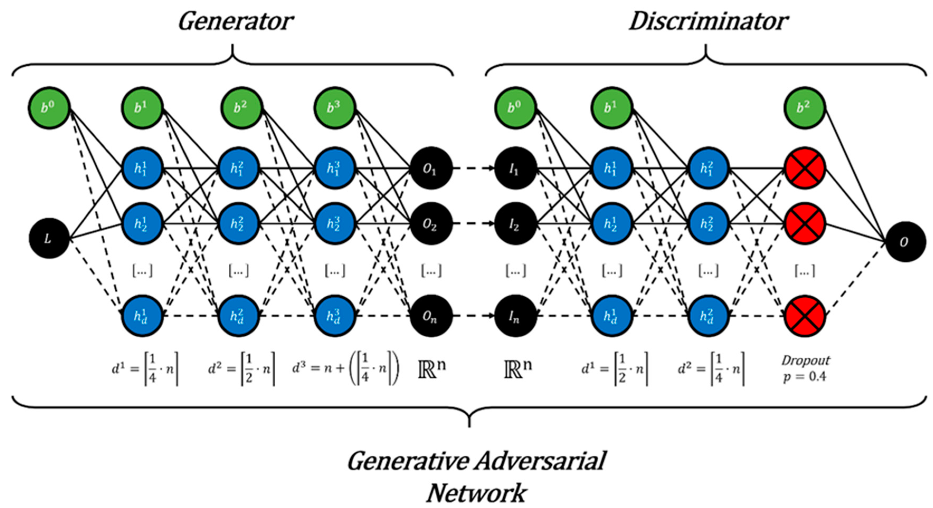
Descriptive figure presenting the optimal GAN architecture for geometric morphometric data augmentation. Input (I) and output (O) neurons are represented in black with bias (b) in green. The output of the generator and the input of the discriminator is represented by the n number of dimensions in the ℝn dimensional target feature space. The latent vector (L) input for the generator must be adjusted according to the dimensionality of the target feature space. Hidden neurons (h) in layers hn have a density (d) that is also conditioned by the shape of the target distribution. Finally, the discriminator has an additional dropout layer (red) with a threshold of p = 0.4.
Figure 4.
Descriptive figure presenting the optimal GAN architecture for geometric morphometric data augmentation. Input (I) and output (O) neurons are represented in black with bias (b) in green. The output of the generator and the input of the discriminator is represented by the n number of dimensions in the ℝn dimensional target feature space. The latent vector (L) input for the generator must be adjusted according to the dimensionality of the target feature space. Hidden neurons (h) in layers hn have a density (d) that is also conditioned by the shape of the target distribution. Finally, the discriminator has an additional dropout layer (red) with a threshold of p = 0.4.

Figure 5.
rTOST absolute difference values obtained comparing synthetic data generated over multiple training steps with the original distribution (example of DS3). Upper and lower panels compare different GANs using different sized latent vector inputs to the generator. GANs were trained for 400 epochs with batch sizes of 16. Here 3 training steps are considered an epoch.

Figure 6.
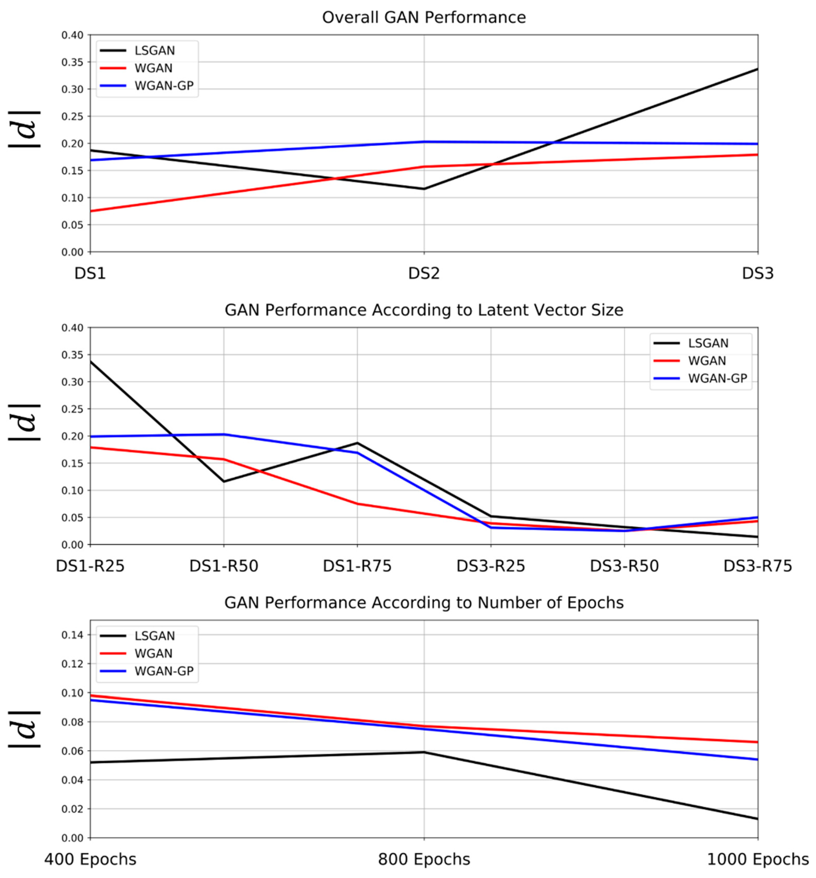
Parallel coordinate plots summarizing contents of Table 3, Table 4, Table 5 and Table 6. Absolute difference values are obtained from robust equivalency testing.

Figure 7.
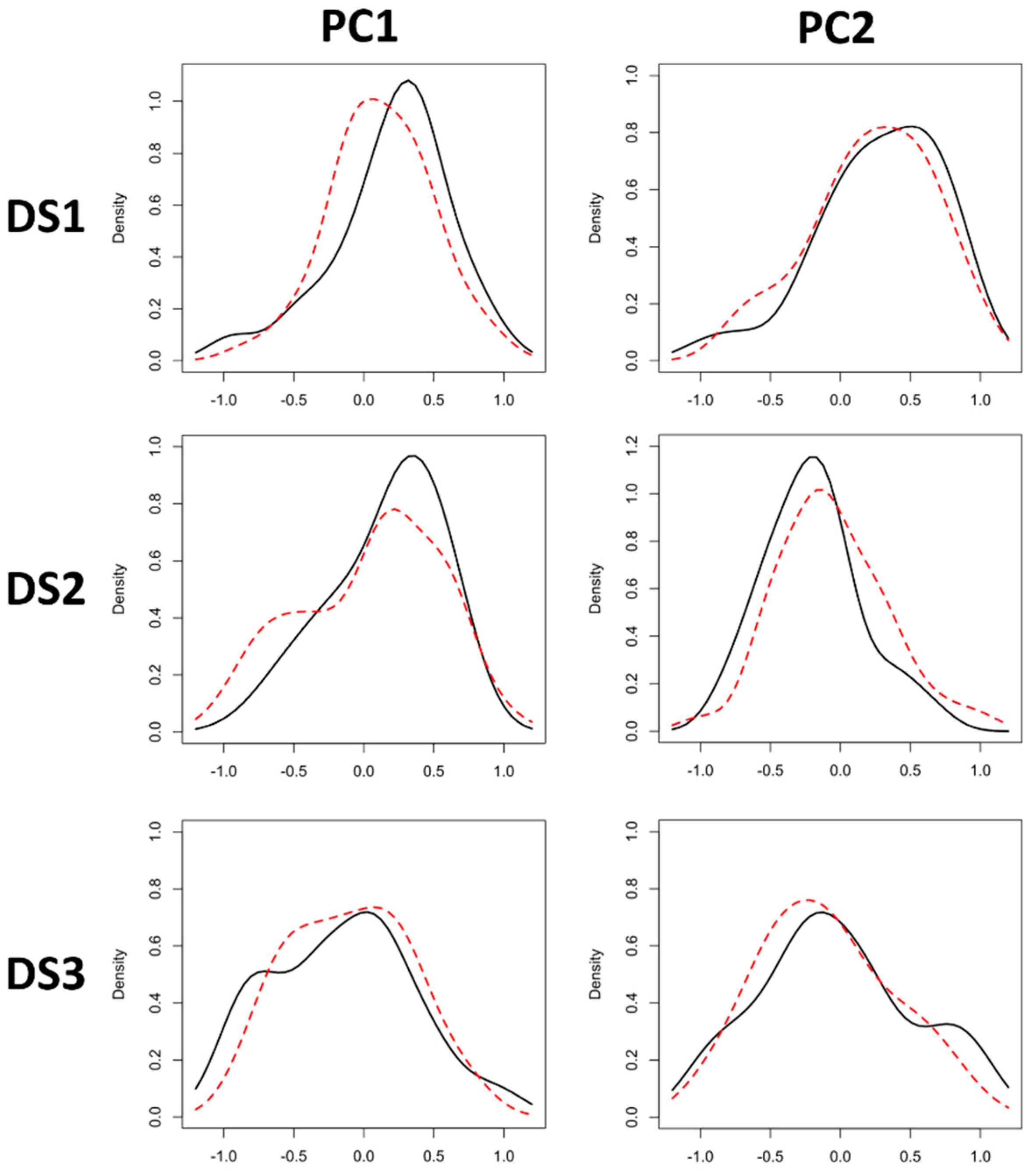
Plots of distributions both before (black) and after (red) GAN data augmentation, using the best performing models as described in Table 3. Descriptive statistics for each are included in Tables S2, S4 and S6.
Figure 7.
Plots of distributions both before (black) and after (red) GAN data augmentation, using the best performing models as described in Table 3. Descriptive statistics for each are included in Tables S2, S4 and S6.

Figure 8.
Histograms and scatter plots of augmented DS3 using bootstrap and GAN. New points are marked in red.
Figure 8.
Histograms and scatter plots of augmented DS3 using bootstrap and GAN. New points are marked in red.

Figure 9.
PCA scatter plot presenting data augmentation techniques on DS3. Ellipses mark 95% confidence intervals. Both CGAN and GAN were trained using Wasserstein Gradient Penalty loss.
Figure 9.
PCA scatter plot presenting data augmentation techniques on DS3. Ellipses mark 95% confidence intervals. Both CGAN and GAN were trained using Wasserstein Gradient Penalty loss.

Figure 10.
Example of the Augmentation (LSGAN ×100) of O’Higgins and Dryden’s Hominoid dataset comparing gorilla (Gorilla gorilla), chimpanzee (Pan troglodytes) and orangutan (Pongo pygmaeus) skulls [75]. (A) Example of both the original and augmented datasets. Percentages next to each group represent the accuracy obtained by a more traditional Linear Discriminant Analysis algorithm. (B) Boxplots presenting the loss and confidence of predictions made using both the original and the augmented data set. To the right Receiver Operator Characteristic curves describe the overall performance of models on both datasets. (C) Decision boundaries drawn by LDA across PC1 (x-axis) and PC2 (y-axis). The upper panel and lower panel of C represent the original and the augmented datasets respectively.


Table 1.
List of hyperparameters and settings tested during optimization of GAN model architectures.
Table 1.
List of hyperparameters and settings tested during optimization of GAN model architectures.
| Hyperparameter | Tested Settings |
|---|---|
| Number of Layers | − |
| Node Density | − |
| Activation Functions | ReLU, Leaky ReLU, Tanh, Swish, ELU, Sigmoid, Linear |
| Kernel Initializer | None, Uniform, Normal and their Random, Truncated or Glorot variants. |
| Dropout | None, Present with thresholds between 0.01 and 0.9 |
| Weight Regularizer | None, l2 with thresholds between 0.01 and 0.0001 |
| Weight Constraint | UnitNorm, MaxNorm, MinMaxNorm |
| Batch Normalization | Present, Absent |
| Training Epochs | Between 100 and 2000 |
| Batch Size | 4, 8, 16, 32 |
| Optimizers | Adam, RMSprop, Stochastic Gradient Descent. Adagrad |
| Learning Rate | Between 0.1 and 0.00001 |
| Decay | Between 0.9 and 0.0001 |
| Momentum | Between 0.99 and 0.1 |
| Loss | Binary cross-entropy, Mean Squared Error, Least Squares, Wasserstein Loss, Wasserstein Gradient Penalty Loss. |
Table 2.
Summary of each dataset’s target domain with univariate calculations of distribution normality in the top two PC scores.
Table 2.
Summary of each dataset’s target domain with univariate calculations of distribution normality in the top two PC scores.
| Domain Dimensionality | PCs with 95% Cumulative Variance | PC1 | PC2 | |||
|---|---|---|---|---|---|---|
| Variance (%) | Shapiro Test w (p) | Variance (%) | Shapiro Test w (p) | |||
| DS1 | ℝ14 | 4 | 69.92 | 0.95 (0.02) | 14.37 | 0.97 (0.15) |
| DS2 | ℝ39 | 11 | 32.27 | 0.96 (0.05) | 25.70 | 0.98 (0.31) |
| DS3 | ℝ60 | 13 | 32.83 | 0.99 (0.75) | 19.55 | 0.98 (0.30) |
Table 3.
Best obtained absolute difference and p value calculations for robust equivalency testing of each of the synthesized distributions using different GANs.
Table 3.
Best obtained absolute difference and p value calculations for robust equivalency testing of each of the synthesized distributions using different GANs.
| LSGAN | WGAN | WGAN-GP | ||||
|---|---|---|---|---|---|---|
| |d| | p | |d| | p | |d| | p | |
| DS1 | 0.187 | 0.0105 | 0.075 | 2.9 × 10⁻⁶ | 0.169 | 0.0013 |
| DS2 | 0.019 | 2.2 × 10⁻¹⁶ | 0.043 | 1.3 × 10⁻¹¹ | 0.002 | 2.1 × 10⁻²⁰ |
| DS3 | 0.052 | 7.3 × 10⁻²⁰ | 0.040 | 6.7 × 10⁻²³ | 0.031 | 3.6 × 10⁻²² |
Table 4.
Best obtained absolute difference and p value calculations for robust equivalency testing. Values calculated comparing the original target distribution (DS1) with synthetic data generated by different GANs with different sized latent vectors as generator input.
Table 4.
Best obtained absolute difference and p value calculations for robust equivalency testing. Values calculated comparing the original target distribution (DS1) with synthetic data generated by different GANs with different sized latent vectors as generator input.
| LSGAN | WGAN | WGAN-GP | ||||
|---|---|---|---|---|---|---|
| |d| | p | |d| | p | |d| | p | |
| ℝ25 | 0.337 | 0.726 | 0.179 | 0.014 | 0.199 | 0.017 |
| ℝ50 | 0.116 | 2.0×10⁻⁴ | 0.157 | 0.004 | 0.203 | 0.026 |
| ℝ75 | 0.187 | 0.0105 | 0.075 | 2.9 × 10⁻⁶ | 0.169 | 0.0013 |
Table 5.
Best obtained absolute difference and p value calculations for robust equivalency testing. Values calculated comparing the original target distribution (DS3) with synthetic data generated by different GANs with different sized latent vectors as generator input.
Table 5.
Best obtained absolute difference and p value calculations for robust equivalency testing. Values calculated comparing the original target distribution (DS3) with synthetic data generated by different GANs with different sized latent vectors as generator input.
| LSGAN | WGAN | WGAN-GP | ||||
|---|---|---|---|---|---|---|
| |d| | p | |d| | p | |d| | p | |
| ℝ25 | 0.052 | 7.3 × 10⁻²⁰ | 0.039 | 6.7 × 10⁻²³ | 0.031 | 3.6 × 10⁻²² |
| ℝ50 | 0.032 | 1.7 × 10⁻²⁴ | 0.025 | 2.6 × 10⁻²⁵ | 0.025 | 1.0 × 10⁻²³ |
| ℝ75 | 0.014 | 1.2 × 10⁻²⁵ | 0.043 | 3.9 × 10⁻²² | 0.050 | 2.4 × 10⁻²⁰ |
Table 6.
Best obtained absolute difference and p value calculations for robust equivalency testing after x number of epochs. Example of GANs trained on a subset of 30 individuals from DS2.
Table 6.
Best obtained absolute difference and p value calculations for robust equivalency testing after x number of epochs. Example of GANs trained on a subset of 30 individuals from DS2.
| Results Obtained after x Epochs | LSGAN | WGAN | WGAN-GP | |||
|---|---|---|---|---|---|---|
| |d| | p | |d| | p | |d| | p | |
| 400 | 0.052 | 6.0 × 10⁻¹⁶ | 0.098 | 2.4 × 10⁻¹² | 0.095 | 3.8 × 10⁻¹² |
| 800 | 0.059 | 3.3 × 10⁻¹⁵ | 0.077 | 9.4 × 10⁻¹³ | 0.075 | 6.02 × 10⁻¹³ |
| 1000 | 0.013 | 3.8 × 10⁻²² | 0.066 | 1.5 × 10⁻¹⁸ | 0.054 | 5.0 × 10⁻¹⁶ |
Table 7.
Comparison of descriptive statistics obtained when comparing traditional bootstrapping procedures for numeric data augmentation and the best performing GAN on DS3. Dataset was augmented to size 100.
Table 7.
Comparison of descriptive statistics obtained when comparing traditional bootstrapping procedures for numeric data augmentation and the best performing GAN on DS3. Dataset was augmented to size 100.
| Original Data | Bootstrap | GAN | ||||
|---|---|---|---|---|---|---|
| PC1 | PC2 | PC1 | PC2 | PC1 | PC2 | |
| Shapiro w | 0.99 | 0.98 | 0.98 | 0.98 | 0.99 | 0.98 |
| Shapiro p | 0.75 | 0.30 | 0.25 | 0.18 | 0.92 | 0.10 |
| Central Tendency ‡ | −0.10 | −0.16 | −0.14 | −0.21 | −0.06 | −0.04 |
| Deviation § | 0.41 | 0.43 | 0.40 | 0.43 | 0.41 | 0.49 |
| Minimum Value | −1.00 | −1.00 | −1.00 | −1.00 | −1.00 | −1.00 |
| IR 0.05 Limit | −0.81 | −0.98 | −0.81 | −0.99 | −0.78 | −0.85 |
| IR 0.95 Limit | 0.47 | 0.61 | 0.47 | 0.52 | 0.55 | 0.84 |
| Maximum Value | 1.00 | 1.00 | 1.00 | 1.00 | 1.00 | 1.00 |
| Kurtosis | −0.33 | 0.19 | −0.43 | −0.24 | −0.49 | −0.65 |
| Skewness | −0.02 | 0.35 | −0.01 | 0.21 | 0.05 | 0.18 |
‡ Metric used = mean; § Metric used = standard deviation.
Table 8.
Best obtained absolute difference and p value calculations for robust equivalency testing when comparing targeted generation of data using CGAN and GAN on DS3. Both CGAN and GAN were trained using Wasserstein Gradient Penalty loss.
Table 8.
Best obtained absolute difference and p value calculations for robust equivalency testing when comparing targeted generation of data using CGAN and GAN on DS3. Both CGAN and GAN were trained using Wasserstein Gradient Penalty loss.
| Sample 1 | Sample 2 | |||
|---|---|---|---|---|
| |d| | p | |d| | p | |
| CGAN | −0.100 | 1.3 × 10⁻⁸ | −0.035 | 2.0 × 10⁻¹⁰ |
| GAN | −0.039 | 2.0 × 10⁻¹⁰ | −0.074 | 2.9 × 10⁻¹⁰ |
Table 9.
Descriptive statistics for augmented DS3 targeting label values specifically. Numbers marked in bold indicate the synthetic data that obtained the most significant rTOST equivalency p-values. Both CGAN and GAN were trained using Wasserstein Gradient Penalty loss.
Table 9.
Descriptive statistics for augmented DS3 targeting label values specifically. Numbers marked in bold indicate the synthetic data that obtained the most significant rTOST equivalency p-values. Both CGAN and GAN were trained using Wasserstein Gradient Penalty loss.
| Original Data | CGAN | GAN | |||||
|---|---|---|---|---|---|---|---|
| PC1 | PC2 | PC1 | PC2 | PC1 | PC2 | ||
| Sample 1 | Shapiro w | 0.98 | 0.97 | 0.97 | 0.97 | 0.98 | 0.98 |
| Shapiro p | 0.75 | 0.59 | 0.25 | 0.25 | 0.31 | 0.31 | |
| Central Tendency ‡ | −0.03 | −0.33 | −0.14 | −0.26 | 0.003 | −0.21 | |
| Deviation § | 0.43 | 0.37 | 0.41 | 0.42 | 0.47 | 0.34 | |
| Minimum Value | −0.87 | −1.00 | −0.89 | −1.00 | −0.87 | −1.00 | |
| IR 0.05 Limit | −0.79 | −0.99 | −0.81 | −0.98 | −0.79 | −0.98 | |
| IR 0.95 Limit | 0.64 | 0.13 | 0.47 | 0.52 | 0.69 | 0.22 | |
| Maximum Value | 1.00 | 0.52 | 1.00 | 0.66 | 1.00 | 0.62 | |
| Kurtosis | −0.44 | −0.49 | −0.49 | −0.53 | −0.97 | 0.20 | |
| Skewness | 0.06 | −0.09 | 0.12 | 0.34 | −0.02 | −0.20 | |
| Sample 2 | Shapiro w | 0.98 | 0.97 | 0.98 | 0.97 | 0.97 | 0.98 |
| Shapiro p | 0.70 | 0.43 | 0.61 | 0.13 | 0.20 | 0.28 | |
| Central Tendency ‡ | −0.17 | 0.01 | −0.08 | 0.19 | −0.14 | 0.03 | |
| Deviation § | 0.38 | 0.44 | 0.43 | 0.46 | 0.50 | 0.40 | |
| Minimum Value | −1.00 | −0.85 | −1.00 | −0.85 | −1.00 | −0.85 | |
| IR 0.05 Limit | −0.81 | −0.59 | −0.78 | −0.59 | −0.85 | −0.55 | |
| IR 0.95 Limit | 0.43 | 0.85 | 0.51 | 0.85 | 0.75 | 0.81 | |
| Maximum Value | 0.47 | 1.00 | 0.92 | 1.00 | 0.97 | 1.00 | |
| Kurtosis | −0.78 | −0.23 | −0.58 | −1.00 | −0.79 | −0.46 | |
| Skewness | −0.28 | 0.42 | 0.18 | −0.14 | 0.31 | 0.39 | |
‡ Metric used = mean; § Metric used = standard deviation.
Publisher’s Note: MDPI stays neutral with regard to jurisdictional claims in published maps and institutional affiliations. |
© 2020 by the authors. Licensee MDPI, Basel, Switzerland. This article is an open access article distributed under the terms and conditions of the Creative Commons Attribution (CC BY) license (http://creativecommons.org/licenses/by/4.0/).
Share and Cite
MDPI and ACS Style
Courtenay, L.A.; González-Aguilera, D. Geometric Morphometric Data Augmentation Using Generative Computational Learning Algorithms. Appl. Sci. 2020, 10, 9133. https://0-doi-org.brum.beds.ac.uk/10.3390/app10249133
AMA Style
Courtenay LA, González-Aguilera D. Geometric Morphometric Data Augmentation Using Generative Computational Learning Algorithms. Applied Sciences. 2020; 10(24):9133. https://0-doi-org.brum.beds.ac.uk/10.3390/app10249133
Chicago/Turabian StyleCourtenay, Lloyd A., and Diego González-Aguilera. 2020. "Geometric Morphometric Data Augmentation Using Generative Computational Learning Algorithms" Applied Sciences 10, no. 24: 9133. https://0-doi-org.brum.beds.ac.uk/10.3390/app10249133
Note that from the first issue of 2016, this journal uses article numbers instead of page numbers. See further details here.