Assessment of Wide-Sense Stationarity of an Underwater Acoustic Channel Based on a Pseudo-Random Binary Sequence Probe Signal

Featured Application

The method described can be used to assess whether the signal received in the underwater acoustic communication system can be modelled as a stochastic wide-sense stationary process. The fulfillment of this condition is necessary both to calculate the basic transmission parameters of the communication channel, such as coherence bandwidth and coherence time, and to correctly detect information transmitted in a UAC systems using modern modulation and coding schemes, such as orthogonal frequency-division multiplexing or spread spectrum techniques. A fast and energy efficient method of assessing whether the received signal meets the WSS assumption can be implemented in a UAC adaptive system, enabling the change of modulation parameters, in particular, the duration of the modulation symbol for which the WSS assumption is fulfilled, thereby increasing the UAC system’s reliability.

Abstract

The performances of Underwater Acoustic Communication (UAC) systems are strongly related to the specific propagation conditions of the underwater channel. Designing the physical layer of a reliable data transmission system requires a knowledge of channel characteristics in terms of the specific parameters of the stochastic model. The Wide-Sense Stationary Uncorrelated Scattering (WSSUS) assumption simplifies the stochastic description of the channel, and thus the estimation of its transmission parameters. However, shallow underwater channels may not meet the WSSUS assumption. This paper proposes a method for testing the Wide-Sense Stationary (WSS) part of the WSSUS feature of a UAC channel on the basis of the complex envelope of a received probe Pseudo-Random Binary Sequence (PRBS) signal. Two correlation coefficients are calculated that can be interpreted, together, as a measure that determines whether the channel is WSS or not. A similar wide-sense stationarity assessment can be performed on the basis of the Time-Varying Impulse Response (TVIR) of a UAC channel. However, the method proposed in this paper requires fewer computational operations in the receiver of a UAC system. PRBS signal transmission tests were conducted in the UAC channel simulator and in real conditions during an inland water experiment. The correlation coefficient values obtained using the method based on the envelope of a probe signal and the method of analysing the TVIR estimates are compared. The results are similar, and thus, it is possible to assess if the UAC channel can be modelled as a WSS stochastic process without the need for TVIR estimation.

1. Introduction

Shallow underwater acoustic communication channels are characterised by disadvantageous transmission properties. Reflections from the sea-bottom and the water’s surface cause multipath propagation, which goes hand-in-hand with the refraction phenomenon, caused by a significant change in sound velocity as a function of depth [1]. The movement of the UAC system’s transmitter and receiver causes a Doppler effect, resulting in the time-domain scaling of a broadband communication signal. Moreover, UAC channel propagation conditions can change over time [2]. Depending on the phenomena under consideration, the variability of the transmission properties can be in the order of several months (i.e., seasons), several days and hours (i.e., tides, times of day), minutes (i.e., internal waves), a few seconds (i.e., surface waves), or milliseconds.

The transmission properties of a shallow UAC channel can be fully described by its time-varying impulse response, measured commonly by a correlation method, and modelled as a tapped delay line $h(t,\tau )$ [3]. A single realisation of $h(t,\tau )$ is defined in a window of observation time t and delay $\tau$. The impulse response $h(t,\tau )$ can be treated as a two-dimensional stationary random process that fulfils the WSSUS assumption. Then, it is possible to calculate the 2-dimensional scattering function $S(\tau ,\nu )={\int }_{\Delta t}{\int }_{\Delta f}{R}_h(\Delta t,\Delta f)e^{-j2\pi (\nu \Delta t-\tau \Delta f)d\Delta td\Delta f}$, where $R_h(\Delta \tau ,\Delta f)$ is the space-time-frequency correlation function of the channel, obtained on the basis of $h(t,\tau )$. It is the basis for calculation of the transition parameters; namely, multipath delay spread ${\tau }_M$, Doppler spread ${\nu }_M$, coherence time $T_C$, and coherence bandwidth $B_C$ [4].

As it is shown in [5], UAC channels are hardly ever WSSUS, and thus the transmission parameters can be determined only in a restricted period of time, and in a limited frequency range. Determining the time interval wherein the second-order statistics of impulse response are independent of time is important for the performance of communication systems working in nonstationary conditions. Only within this time interval is it possible to calculate transmission parameters $\{{\tau }_M,T_C,{\nu }_M,B_C\}$. Moreover, within this time interval, the signal received by the UAC system receiver represents a WSS process, and its power spectrum can be defined via a Fourier transform, according to the Wiener-Khinchin Theorem. This is especially important for signal detection performed in the frequency domain, as is the case with communication systems using the Orthogonal Frequency-Division Multiplexing (OFDM), and the Frequency Hopping Spread Spectrum (FHSS) techniques [4,6,7].

Studies on the validity of the WSS assumption are relatively rare. Several authors have proposed methods designed to test the similarity of the spectral properties of a time-series [8,9]. The relationship between the radiocommunication signal bandwidth and the wireless channel stationarity is described in [10]. The stationarity of a UAC channel was studied in [11]. The authors described the influence of the wind-driven surface wave variability on fluctuations of the channel Power Spectral Density (PSD). A trend-stationary channel model was proposed in [12] for underwater communication system. In [13], the stationarity of PSD is analysed to verify if the UAC channel can be considered to be a WSS process. Most of these methods are based on spectral analysis.

In [14], a novel time-domain method for verifying the WSS feature of UAC channels is described. Statistical properties of the real and imaginary parts of the impulse response, measured using the correlation method, are exploited to test the WSS assumption fulfilment. In [6] a similar method is proposed to assess whether the channel is WSS/non-WSS on the basis of the complex envelope of a received probe signal. However, the method was tested only in simulation conditions.

In this paper, both methods are compared using the results of simulations and the inland water experiment. The values of correlation coefficients, which are the basis of the WSS indicator proposed in [6], are presented. These coefficients express the similarity of the autocorrelation and cross-correlation functions of the in-phase and quadrature components of the received signal and the impulse response estimated using this signal. However, the calculation of the TVIR requires performing matched filtration in the receiver, which in the case of long impulse responses, measured using dozens of repetitions of a single probe sequence, is time and energy consuming. The simulation and experimental tests have confirmed that a decision can be made if the UAC channel fulfils the WSS assumption on the basis of the analysis of the complex envelope of the received probe signal, instead of the analysis of TVIR of the channel. Skipping the TVIR calculation stage can significantly reduce the processing time and power consumption of the UAC receiver.

2. UAC Impulse Response Measurement

The UAC channel impulse response measurements are usually performed by the correlation method with the use of probe signal having an impulse-like autocorrelation function [15]. One of these signals is a pseudo-random binary sequence (PRBS) being a repetition of a bipolar m-sequence $c_m\in \{-1;1\}$, modulated onto a binary phase-shift keyed waveform $s\left(t\right)=\mathrm{Re}\left[x\left(t\right)e^{j2\pi f_{0}t}\right]$, and $x\left(t\right)$ can be denoted as:

$$x\left(t\right)=\sum _{m=0}^{M-1}{c}_{m}rect(t-\frac{m}{M}T)$$

(1)

where $T=1/B$, B is the signal bandwidth, $f_c$ is the carrier frequency, and the sequence length $M=2^L-1$ is determined by its order L. The $rect\left(t\right)$ denotes the rectangular function. The probe signal is constructed of K subsequent sequences $s\left(t\right)$, each of duration $T_s$, without any pause in between. To produce signal $s\left(t\right)$, m-sequence $c_m$ is upsampled by a factor $R=f_s/B$. Next, the signal is passed through a binary phase shift keying (BPSK) block and it modulates the carrier frequency $f_c$.

At the receiver the analog signal from the ultrasonic transducer is digitised by an analog-to-digital converter. After demodulation, the signal is passed through a matched filter with coefficients corresponding to the upsampled m-sequence used in the transmitter. The matched filtration algorithm is usually implemented in a frequency domain, using a discrete Fourier transform (DFT) [16]. As a result, at each observation time t, a single realisation of the time-varying impulse response $h(t,\tau )$ is obtained.

3. Testing Wide-Sense Stationary Assumption Fulfilment

A random process is wide-sense stationary if its mean value and its autocorrelation function are time invariant. The relation between the WSS bandpass process $r\left(t\right)$, and its complex envelope $y\left(t\right)$, has been described in [17] as:

$$r\left(t\right)=\mathrm{Re}\left[y\left(t\right)e^{j2\pi f_{0}t}\right]=\frac{1}{2}y\left(t\right)e^{j2\pi f_{0}t}+\frac{1}{2}{y}^{*}\left(t\right)e^{-j2\pi f_{0}t}$$

(2)

The complex envelope $y\left(t\right)$ must be a zero-mean process in order that $E\left[r\right(t\left)\right]$ be independent of t. Moreover, the autocorrelation function $R_{rr}(t+\Delta t,t)=E\left[r(t+\Delta t)r\left(t\right)\right]$ of bandpass signal $r\left(t\right)$ is related to its complex envelope $y\left(t\right)$ in the following manner:

$$R_{rr}(t+\Delta t,t)=\frac{1}{2}\mathrm{Re}\left[R_{yy}(\Delta t)e^{\alpha (\Delta t)}\right]+\frac{1}{2}\mathrm{Re}\left[R_{yy*}(\Delta t)e^{j\alpha (\Delta t)+j\beta \left(t\right)}\right]$$

(3)

where $\alpha (\Delta t)=2\pi f_0\Delta t$, $\beta \left(t\right)=4\pi f_{0}t$, $R_{yy}(\Delta t)=E\left[y(t+\Delta t)y^{*}\left(t\right)\right]$, and $R_{y{y}^{*}}(\Delta t)=E\left[y(t+\Delta t)y\left(t\right)\right]$. If $r\left(t\right)$ is WSS, then the t-dependent term in Equation (3) vanishes; i.e., $R_{y{y}^{*}}(\Delta t)=0$. The process $y\left(t\right)=I\left(t\right)+jQ\left(t\right)$ is a complex value; thus, $R_{y{y}^{*}}(\Delta t)$ can be rewritten as:

$$R_{y{y}^{*}}(\Delta t)=R_{II}(\Delta t)-R_{QQ}(\Delta t)+j[R_{IQ}(\Delta t)+R_{QI}(\Delta t)]$$

(4)

where $R_{II}(\Delta t)=E\left[I(t+\Delta t)I\left(t\right)\right]$ and $R_{QQ}(\Delta t)=E\left[Q(t+\Delta t)Q\left(t\right)\right]$ are the autocorrelation functions of $I\left(t\right)$ and $Q\left(t\right)$, and $R_{IQ}(\Delta t)=E\left[I(t+\Delta t)Q\left(t\right)\right]$ and $R_{QI}(\Delta t)=E\left[Q(t+\Delta t)I\left(t\right)\right]$ are their cross-correlation functions. Thus, the condition for wide-sense stationarity of bandpass signal $r\left(t\right)$ requires that:

$$R_{II}(\Delta t)=R_{QQ}(\Delta t)\mathrm{and}{R}_{IQ}(\Delta t)=-R_{QI}(\Delta t)$$

(5)

Moreover, the complex envelope $y\left(t\right)$ should be a zero-mean process. According to [6], the similarity of autocorrelation functions $R_{II}(\Delta t,\tau )$ and $R_{QQ}(\Delta t,\tau )$ can be expressed as the cross-correlation coefficient:

$$c_{IQ}=\underset{\Delta t^{\prime }}{max}\left[E[R_{II}(\Delta t+\Delta t^{\prime }),R_{QQ}(\Delta t)]\right]$$

(6)

and similarity of cross-correlation functions $R_{IQ}(\Delta t,\tau )$ and $R_{QI}(\Delta t,\tau )$, can be described as coefficient:

$$c_{IQQI}=\underset{\Delta t^{\prime }}{max}\left[E[R_{IQ}(\Delta t+\Delta t^{\prime }),-R_{QI}(\Delta t)]\right]$$

(7)

In [14] the method of testing, if the impulse response measured with the probe signal $s\left(t\right)$ satisfies the assumption of WSS, it is presented. It is based on testing the similarity of the autocorrelation functions: $R_{II}^h(\Delta t,\tau )=E\left[h_I(t+\Delta t,\tau )h_I(t,\tau )\right]$, $R_{QQ}^h(\Delta t,\tau )=E\left[h_Q(t+\Delta t,\tau )h_Q(t,\tau )\right]$, and cross-correlation functions: $R_{IQ}^h(\Delta t)=E\left[h_I(t+\Delta t,\tau )h_Q(t,\tau )\right]$, $R_{QI}^h(\Delta t)=E\left[h_Q(t+\Delta t,\tau )h_I(t,\tau )\right]$, defined similarly as in Equations (6) and (7) for in-phase $h_I(t,\tau )$ and quadrature $h_Q(t,\tau )$ components of the impulse response $h(t,\tau )$. The cross-correlation coefficients $c_{IQ}^h$ and $c_{IQQI}^h$ are calculated as functions of delay $\tau$:

$$c_{IQ}^h\left(\tau \right)=\underset{\Delta t^{\prime }}{max}\left[E[R_{II}^h(\Delta t+\Delta t^{\prime },\tau ),R_{QQ}^h(\Delta t,\tau )]\right]$$

(8)

$$c_{IQQI}^h\left(\tau \right)=\underset{\Delta t^{\prime }}{max}\left[E[R_{IQ}^h(\Delta t+\Delta t^{\prime },\tau ),-R_{QI}^h(\Delta t,\tau )]\right]$$

(9)

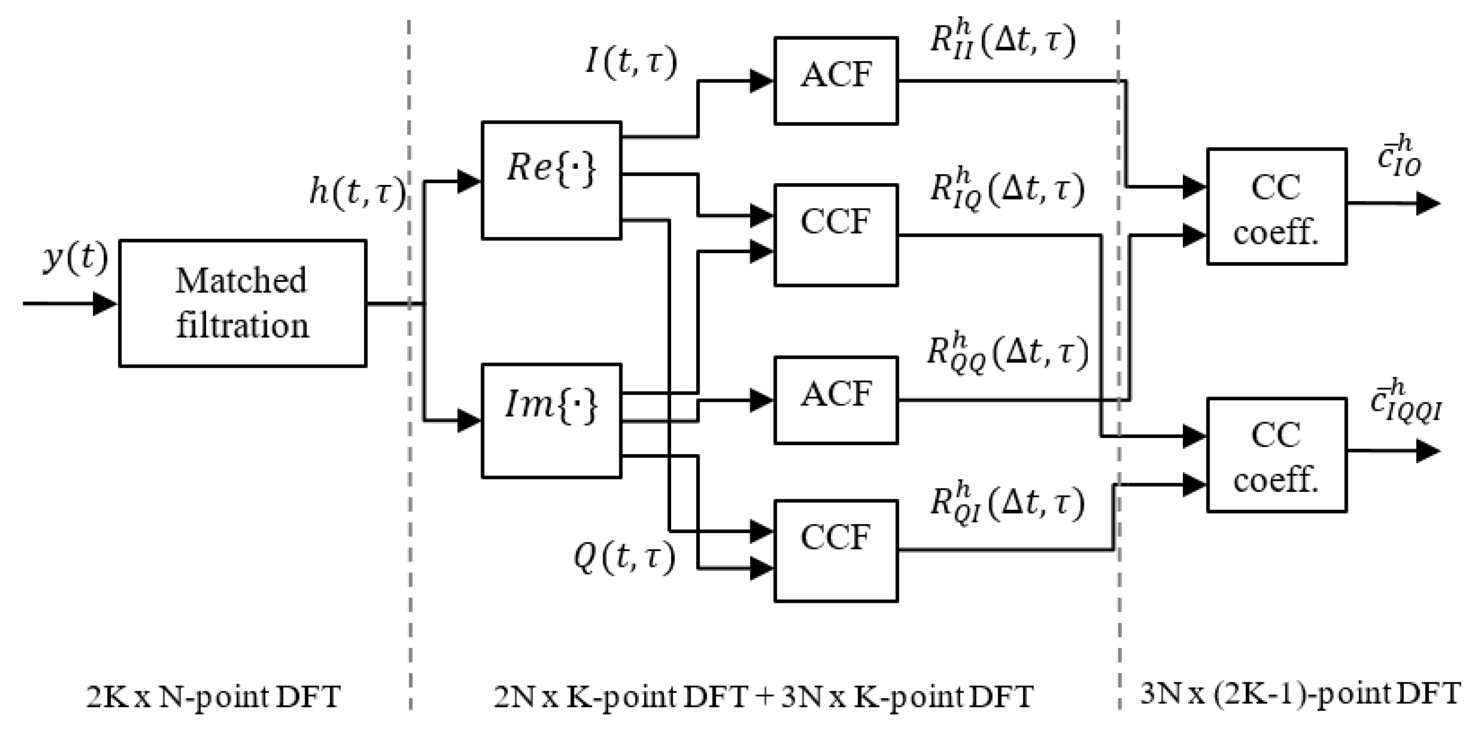
For each TVIR, mean values of these coefficients can be obtained as: ${\overline{c}}_{IQ}^h=E\left[c_{IQ}^h\left(\tau \right)\right]$ and ${\overline{c}}_{IQQI}^h=E\left[c_{IQQI}^h\left(\tau \right)\right]$. The calculation of these coefficients requires the calculation of the TVIR estimate first. As mentioned in Section 2, the DFT transform is usually used to implement the matched filtering algorithm. As it is shown in Figure 1, to calculate K realisations of $h(t,\tau )$, each of which has N samples, the N-point DFT algorithm should be run $2K$ times.To be more precise, one DFT is used for frequency domain transition, and one inverse DFT is needed to return to the time domain. Next, the autocorrelation functions (ACFs): $R_{II}^h$ and $R_{QQ}^h$, and cross-correlation functions (CCFs): $R_{IQ}^h$ and $R_{QI}^h$ are also calculated using DFT. There are $2N$ calls of K-point DFT in the case of calculation of ACFs, and $3N$ calls of DFT of the same size in the case of calculation of CCFs. The difference is due to the fact that in the case of ACF, the DFT is calculated for one input vector, and in the case of CCF, it is calculated for two different input vectors. In order to determine the correlation coefficients, $3N$ DFT calls are needed, each of the size $2K-1$, resulting from the size of input ACFs and CCFs. In the case of calculating the $c_{IQ}$ and $c_{IQQI}$ coefficients directly from the complex envelope $y\left(t\right)$ of the received signal, the matched filtering step is omitted and there is $2K$ of N-point DFTs less to calculate.

4. Results

Simulation and experimental tests have been performed in order to compare the values of $\{c_{IQ},c_{IQQI}\}$ coefficients calculated on the basis of probe PRBS signal and $\{{\overline{c}}_{IQ}^h,{\overline{c}}_{IQQI}^h\}$ coefficients calculated on the basis of measured impulse response.

4.1. Simulation Tests

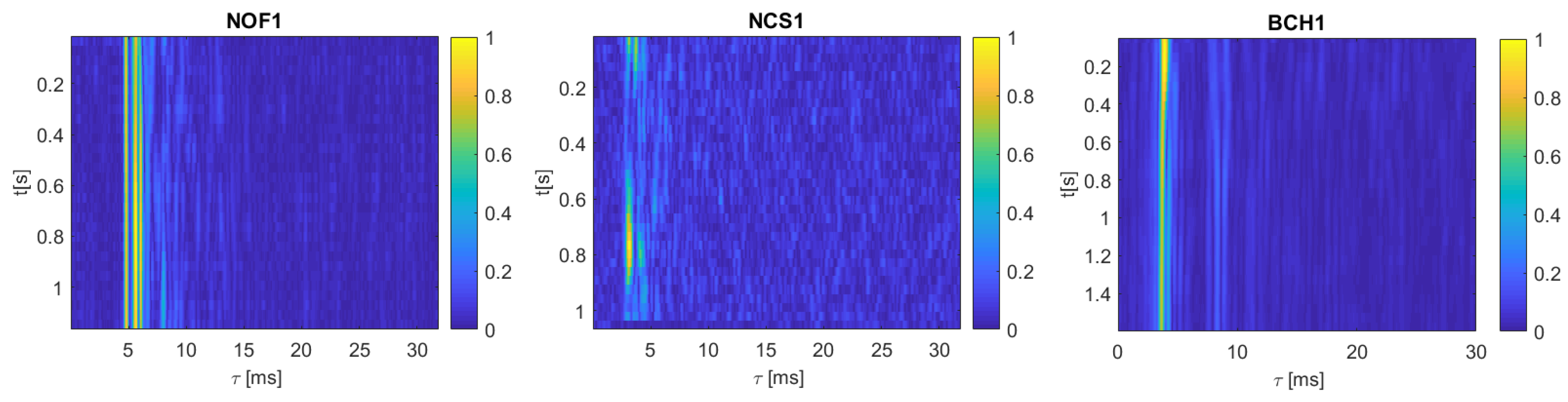
The simulation tests were performed using the Watermark simulator. It is a freely available benchmark for physical-layer schemes for underwater acoustic communications [18]. Its core is a replay channel simulator driven by at-sea measurements of the time-varying impulse response. Three of the communication channels available in Watermark were selected, represented by impulse responses measured in: Norway-Oslofjord (NOF1), Norway-Continental Shelf (NCS1), and Brest Commercial Harbor (BCH1). The NOF1 channel was measured at a range of 750 m and the water depth was 10 m. The probe signal frequency band was 10–18 kHz. The NCS1 channel was measured at a range of 540 m and the water depth was 80 m. The probe signal frequency band was the same as in the case of NOF1 channel measurements. Finally, the BCH1 channel was measured at a range of 800 m, where the water depth was 20 m. The frequency band of the probe signal was 32.5–37.5 kHz. The transmitter was bottom-mounted in the case of NOF1 and NCS1, and suspended in the water column in BCH1. The receiver was a bottom-mounted hydrophone (NOF1, NCS1) or a vertically suspended hydrophone array (BCH1). A more detailed description of Watermark channels can be found in [18]. Figure 2 shows the absolute values of exemplary impulse responses for each channel.

During the simulation tests performed, a PRBS signal was transmitted in the NOF1, NCS1, and BCH1 channels. For the construction of the PRBS signal, m-sequences of order 8 and 10 were used. The spectrum of the signal was in the 10–18 kHz band for the NOF1 and NCS1 channels, and 32.5–37.5 kHz for the BCH1 channel. The sampling frequency was equal to 200 kHz. Sixty transmission tests were carried out for each configuration of the signal and channel parameters. During a single transmission test, the probe sequence was repeated 32 times.

On the basis of the received signals, after performing a matched filtration, TVIR estimates and the corresponding coefficients ${\overline{c}}_{IQ}^h$ and ${\overline{c}}_{IQQI}^h$ were determined. Next, the complex envelope $y\left(t\right)$ of each of the received signal was divided into segments of a duration corresponding to the duration of a single PRBS sequence. The coefficients $c_{IQ}$ and $c_{IQQI}$ were calculated as mean values over all segments of the probe signal. The minimum value of the coefficient is 0, and the maximum is 1. It is assumed that a value of the cross-coefficient above 0.5 means a strong similarity, and below 0.5 a weak similarity. This is consistent with the assumption of a stochastic model of the wireless communication channel, that two received signals are similar if their correlation coefficient is equal or greater than 0.5. This rule applies, inter alia, when calculating coherence time and the coherence bandwidth of the channel as a time interval and a frequency shift, respectively, for which the correlation coefficient of such delayed or frequency-shifted signals is equal or greater than 0.5 [19]. It is reasonable to assume that if values of both cross-coefficients: $c_{IQ}$ and $c_{IQQI}$ are greater than 0.5, the channel can be described as a WSS process.

In order to compare the coefficients obtained for the TVIR and for the complex envelope of the received signal, a euclidean distance measure d was calculated as:

$$d=\sqrt{{({\overline{c}}_{IQ}^h-c_{IQ})}^2+{({\overline{c}}_{IQQI}^h-c_{IQQI})}^2}$$

(10)

It has a meaning of error of estimation of $c_{IQ}$ and $c_{IQQI}$ parameters, assuming that ${\overline{c}}_{IQ}^h$ and ${\overline{c}}_{IQQI}^h$ are the reference values. The distance d was averaged over 60 transmission tests for each channel.

Table 1. Results of simulation tests.

Channel	m-Sequence Order	Bandwidth	Probe Sequence Duration	${\overline{\mathit{c}}}_{\mathit{IQ}}^{\mathit{h}}$	${\mathit{c}}_{\mathit{IQ}}$	${\overline{\mathit{c}}}_{\mathit{IQQI}}^{\mathit{h}}$	${\mathit{c}}_{\mathit{IQQI}}$	d
NOF1	8	8 kHz	32 ms	0.7469	0.6590	0.6790	0.7126	0.0941
NOF1	10	8 kHz	128 ms	0.7414	0.6374	0.6936	0.6748	0.1057
NCS1	8	8 kHz	32 ms	0.6349	0.6114	0.6248	0.6374	0.0267
NCS1	10	8 kHz	128 ms	0.5617	0.5302	0.5842	0.5385	0.0555
BCH1	8	5 kHz	51 ms	0.9165	0.7868	0.8611	0.7988	0.1439
BCH1	10	5 kHz	205 ms	0.8747	0.6916	0.8307	0.7099	0.2194

presents the values of the coefficients calculated on the basis of TVIR, the coefficients obtained on the basis of the envelope of the PRBS signal, and values of distance measure d.

It can be seen that the smallest differences between the correlation coefficients ${\overline{c}}_{IQ}^h$, ${\overline{c}}_{IQQI}^h$, and {$c_{IQ}$, $c_{IQQI}$} were observed for the NCS1 channel, and the largest differences were recorded for the BCH1 channel.

4.2. Underwater Experiment

The inland water channel measurements were conducted on the 4th and 5th of May 2017, in the Wdzydze Lake on the northern edge of the Bory Tucholskie forest complex (53${}^{\circ }$58${}^{\prime }$31${}^{″}$ N 17${}^{\circ }$54${}^{\prime }$19${}^{″}$ E). The bottom of the lake falls steeply into the depths of the water. In the shore zone, it is lined with gravel-stony material, and in the deeper parts, covered with a layer of mud. Wdzydze Lake is in many respects very similar to the Baltic Sea. A significant part of the lake area is more than 40 m deep, and the deepest area is more than 70 m deep. The shape of the bottom of the Wdzydze lake is more diverse than the bottom of the Baltic Sea; thus, the propagation conditions are even more difficult than those in the sea.

The weather was windy and it was raining on the 4th May, when the measurements were performed at a distance of 550 m. The next day, during the measurements at distances of 340 m and 1035 m, the weather was windless; it was not raining and the water surface was calm.

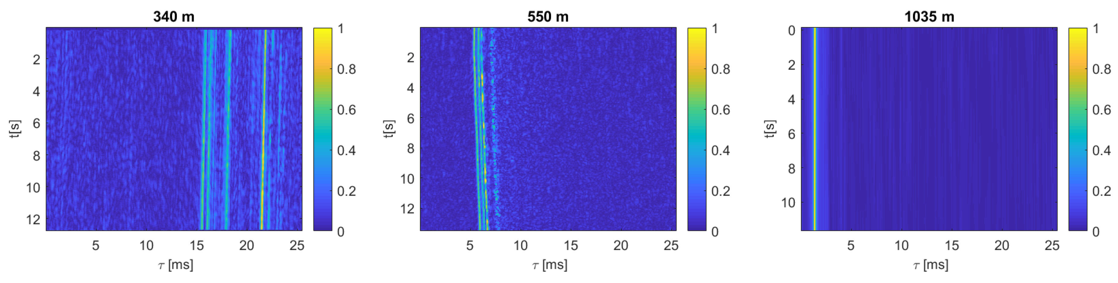
Each probe signal was generated using a computer with MATLAB software. Conversion from digital to analogue signal was performed using a digital-to-analogue converter from an NI USB-6363 device. Next, the signal was amplified and transmitted to water by an underwater telephone HTL-10 [20]. The transmission stand was placed on board the boat. The same equipment was used in the receiving stand, but was configured differently. The boat was not anchored, but drifted very slowly. Therefore, the Doppler effect had an effect on the transmitted signal, but to a much lesser extent than strong multipath propagation. The receiving equipment was placed in a measuring container whose position was fixed. The transmission transducer was sunk to a depth of 10 m, regardless of the water depth of about 20–30 m. The receiving transducer was sunk to a depth of 4 m at a constant water depth of 7 m; thus, even a slight rippling of the water had an effect on the stationarity of the received signal. A more detailed description of the experimental set-up can be found in [21]. Figure 3 shows the absolute values of exemplary impulse responses for each of measured channels.

During the experiment, the PRBS probe signal was transmitted, based on m-sequences of order 8 and 10, repeated 500 times, and occupied frequency bands of 5 kHz, 8 kHz, and 10 kHz. The carrier frequency and the sampling frequency were equal to 30 and 200 kHz, respectively. Due to different propagation conditions and different transmission powers of the measuring system, the received signal to noise ratio (SNR) was different for each of the three measured channels. At a distance of 340 m, the SNR was in the range of 10 to 13 dB; at a distance of 550 m it was in the range of 13 to 18 dB; and at a distance of 1035 m the SNR was in the range of 32 to 35 dB.

On the basis of the received signals, similar to the simulation experiment, after performing a matched filtration, the impulse response estimates were determined. Next, the coefficients ${\overline{c}}_{IQ}^h$, ${\overline{c}}_{IQQI}^h$, were calculated. Simultaneously, the complex envelope $y\left(t\right)$ of each of received signals was divided into segments of duration corresponding to the duration of a single PRBS sequence, and the coefficients $c_{IQ}$ and $c_{IQQI}$ were determined. Next, the values of the distance measure d according to Equation (10) were calculated.

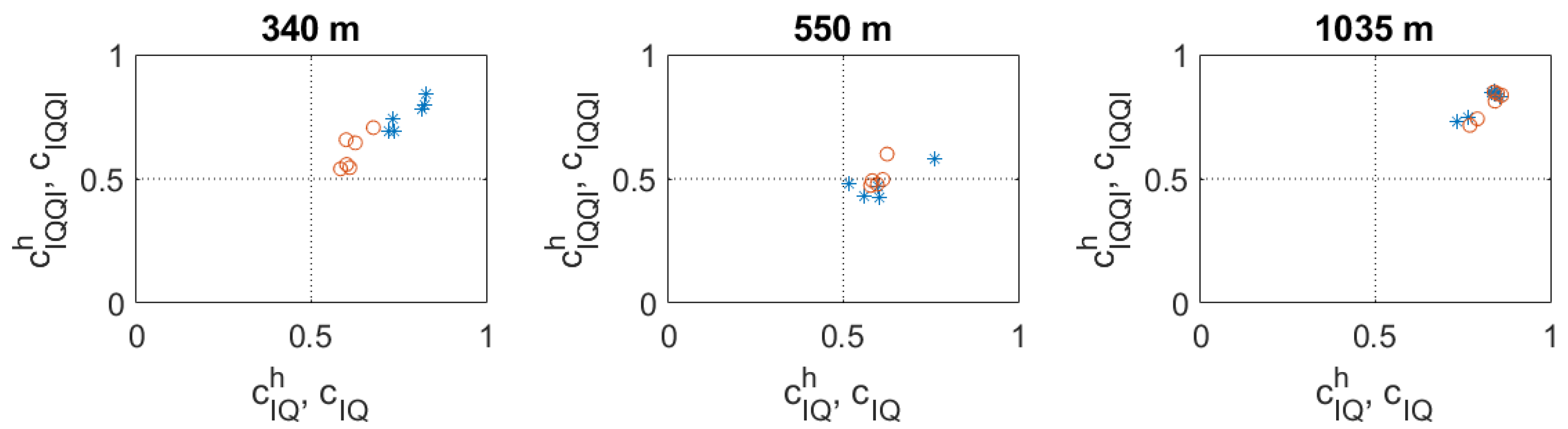
The results of analysis of the transmitted PRBS signals and estimated TVIRs are shown in

Table 2. Results of inland-water experimental tests

Distance [m]	m-Seq. Order	B [kHz]	Probe Seq. Duration [ms]	${\overline{\mathit{c}}}_{\mathit{IQ}}^{\mathit{h}}$	${\mathit{c}}_{\mathit{IQ}}$	${\overline{\mathit{c}}}_{\mathit{IQQI}}^{\mathit{h}}$	${\mathit{c}}_{\mathit{IQQI}}$	d
340	8	5	51.2	0.825 (0.812)	0.678	0.798 (0.798)	0.706	0.173 (0.163)
340	8	8	32.0	0.829 (0.815)	0.626	0.842 (0.837)	0.645	0.283 (0.270)
340	8	10	25.6	0.816 (0.812)	0.600	0.780 (0.787)	0.657	0.249 (0.249)
340	10	5	204.8	0.737 (0.720)	0.601	0.691 (0.674)	0.558	0.190 (0.166)
340	10	8	128.0	0.734 (0.723)	0.610	0.739 (0.733)	0.545	0.231 (0.219)
340	10	10	102.4	0.722 (0.720)	0.584	0.691 (0.693)	0.540	0.204 (0.203)
550	8	5	51.2	0.762 (0.740)	0.625	0.583 (0.548)	0.599	0.138 (0.127)
550	8	8	32.0	0.602 (0.593)	0.597	0.426 (0.413)	0.478	0.052 (0.065)
550	8	10	25.6	0.559 (0.544)	0.613	0.429 (0.405)	0.497	0.087 (0.115)
550	10	5	204.8	0.516 (0.536)	0.583	0.482 (0.428)	0.493	0.067 (0.080)
550	10	8	128.0	0.600 (0.560)	0.578	0.470 (0.425)	0.473	0.022 (0.051)
1035	8	5	51.2	0.830	0.860	0.847	0.837	0.032
1035	8	8	32.0	0.840	0.848	0.852	0.842	0.012
1035	8	10	25.6	0.840	0.839	0.840	0.850	0.009
1035	10	5	204.8	0.856	0.842	0.830	0.812	0.023
1035	10	8	128.0	0.765	0.791	0.749	0.741	0.028
1035	10	10	102.4	0.735	0.770	0.732	0.715	0.039

. As seen in Figure 3 there is a small Doppler shift observed in the impulse responses measured at distances of 340 and 550 m. The impulse responses were resampled to remove the influence of the Doppler effect. The cross correlation coefficients were calculated for both cases: before and after resampling. The values of the coefficients and the distance measure calculated after resampling the TVIR are written in brackets. It is clearly seen that a small Doppler shift due to the drifting of the boat with the transmitting stand does not significantly affect the obtained results. The values of cross-correlation coefficients $\{{\overline{c}}_{IQ}^h,{\overline{c}}_{IQQI}^h\}$, and $\{c_{IQ},c_{IQQI}\}$ are also presented in Figure 4.

As the measurement system range increases, the difference between the cross-correlation coefficients $\{{\overline{c}}_{IQ}^h,{\overline{c}}_{IQQI}^h\}$ and $\{c_{IQ},c_{IQQI}\}$ decreases. At a range of 340 m, the distance measure d is up to 0.28, while for a distance of 1035 m it does not exceed the value of 0.04. At the same time the highest correlation coefficient results were obtained for the channel at a distance of 1035 m. This channel turned out to be the strongest wide-sense stationary. The lowest coefficient results were obtained for the 550 m channel, in which transmission was carried out in bad weather conditions. The $c_{IQQI}$ values below 0.5 do not allow it to be classified as WSS.

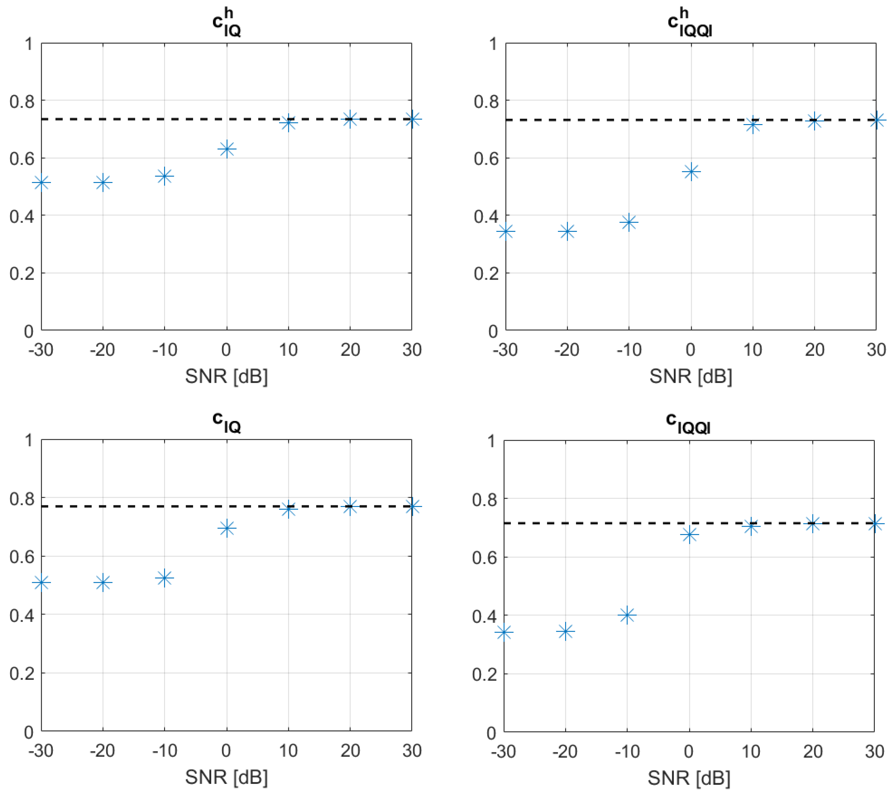
In order to estimate the impact of SNR (which was different during measurements at different distances) on the results obtained, additional simulation tests were performed using the signals measured at a distance of 1035 m (SNR was the largest in this case). Additive Gaussian noise of a different level was added to the signal, and then the correlation coefficients were calculated. The results are shown in Figure 5. It is clearly seen that if the SNR is equal or greater than 10 dB, the effect of additive noise on the calculation results is negligible.

5. Discussion

In the simulation tests carried out, the differences between the pairs of cross-correlation coefficients, $\{{\overline{c}}_{IQ}^h,{\overline{c}}_{IQQI}^h\}$ and $\{c_{IQ},c_{IQQI}\}$, were different depending on the channel tested. The highest distance measurement values (up to 0.22) were obtained for the BCH1 channel, where the transmitting and receiving transducers were suspended in the water. In case of the two other tested channels, namely, NOF1 and NCS1, the transmitting and receiving transducers were bottom-mounted. The distance measure d for NOF1 and NCS1 is less than 0.1. Another difference between the BCH1 and NCS1/NOF1 channels is the fact that in the case of BCH1 channel the ratio of the bandwidth (5 kHz) to the carrier frequency (35 kHz) is 1/7, while in the case of the NCS1 and NOF1 channels, this ratio is equal to 8 kHz/14 kHz = 4/7. Thus, the BCH1 channel is much more narrowband than the two other simulated UAC channels. Assuming that values of cross-correlation coefficients $c_{IQ}$ and $c_{IQQI}$ greater than 0.5 indicate that the channel is WSS, using both pairs of coefficients leads to the same Watermark channels classification results as being WSS.

During the inland water experiment, the largest differences between the pairs of cross-correlation coefficients were obtained for the channel with the smallest range (340 m). In this case the distance measure d was up to 0.28. This channel is characterised by the strongest multipath propagation. In case of the longest range, namely, 1035 m, the distance measure between the coefficients was the lowest (up to 0.039). Both the coefficients ${\overline{c}}_{IQQI}^h$ and $c_{IQQI}$ for the channel measured in bad atmospheric conditions over a distance of 550 m take values of less than 0.5. Thus, the channel was classified as non-WSS.

Assessment of channel wide-sense stationarity based on the coefficients $c_{IQ}$ and $c_{IQQI}$, calculated directly from the complex envelope $y\left(t\right)$ of the received signal, makes it possible to obtain the same classification result as using the coefficients ${\overline{c}}_{IQ}^h$ and ${\overline{c}}_{IQQI}^h$. At the same time, calculating $c_{IQ}$ and $c_{IQQI}$ requires fewer computational operations, due to the fact that the TVIR channel estimation step is omitted.

Table 3. TVIR calculation time and energy consumption for TMS320VC5505 digital signal processor.

m-Seq. Order	Bandwidth [kHz]	K	N	Complex FFT Size	FFT Calc. Time [ms]	TVIR Est. Time [s]	Energy/FFT [μJ]	Energy/TVIR [mJ]
8	5	196	10,200	16,384	4.43	1.74	177.57	69.61
8	8	360	6375	8192	2.22	1.60	88.78	63.92
8	10	450	5100	8192	2.22	2.00	88.78	79.90
10	5	56	40,920	65,536	17.74	1.99	710.27	79.55
10	8	89	25,575	32,768	8.87	1.58	355.13	63.21
10	10	117	20,460	32,768	8.87	2.08	355.13	83.10

shows the sample calculation times and power consumption related to the estimation of the UAC channel TVIR by a fixed-point digital signal processor TMS320VC5505 by Texas Instruments [22]. The size of the impulse response corresponds to the results of measurements obtained during the inland-water experiment at a distance of 1 km. For each impulse response, the size of the complex FFT and the corresponding calculation time and the amount of energy consumed by the processor were determined. The calculation time for each estimate is about 1.5–2 s. In the case of very short range systems, it is longer than the time at which the acoustic wave travels the path between the transmitter and receiver. It may be an undesirable, significant delay in the case of an adaptive UAC system. The signal processor needs 63.21 to 83.10 mJ of energy to estimate the TVIR. If the calculation takes about 2 s, these values correspond to about 30–40 mW of power consumption. In case of the off-the-shelf acoustic modems, the power consumption on the receiving side usually does not exceed 1 W. Thus, every few dozen Watts of less power consumed might be a significant improvement of UAC system power efficiency.

6. Conclusions

An underwater acoustic communication channel can be classified as WSS or non-WSS on the basis of analysis of a baseband, complex value PRBS signal received by the UAC system receiver. If the received signal can be modelled as a WSS stochastic process, then its in-phase and quadrature components have similar autocorrelation functions, and its cross-correlation function is symmetric. The correlation coefficients of these components are being proposed as indicators for assessment of wide-sense stationarity of the UAC channel. Two algorithms of WSS assessment have been compared in this paper. One of them is used to calculate the correlation coefficients on the basis of the TVIR of the channel. The second one skips the TVIR estimation stage, and thus allows the channel to be evaluated with fewer computational operations. Analysis of the results of PRBS signal transmission in the UAC channel under simulation conditions and during an inland water experiment showed that although the two algorithms lead to slightly different values of correlation coefficients, the results of classification of the measured channel as WSS/non-WSS are the same in both cases.

References

- Grelowska, G.; Kozaczka, E.; Witos-Okrasińska, D. Vertical Temperature Stratification of the Gulf of Gdansk Water. In Proceedings of the 2018 Joint Conference—Acoustics, Ustka, Poland, 11–14 September 2018; pp. 80–85. [Google Scholar] [CrossRef]
- Grelowska, G. Study of Seasonal Acoustic Properties of Sea Water in Selected Waters of the Southern Baltic. Pol. Marit. Res. 2016, 23, 25–30. [Google Scholar] [CrossRef] [Green Version]
- van Walree, P. Channel Sounding for Acoustic Communications: Techniques and Shallow-Water Examples; FFI-Rapport 2011/00007; Forsvarets forskningsinstitutt: Kjeller, Norway, 2011. [Google Scholar]
- Kochanska, I.; Schmidt, J.; Rudnicki, M. Underwater Acoustic Communications in Time-Varying Dispersive Channels. In Proceedings of the 2016 Federated Conference on Computer Science and Information Systems (FedCSIS), Gdańsk, Poland, 11–14 September 2016; pp. 467–474. [Google Scholar]
- Nissen, I.; Kochanska, I. Stationary underwater channel experiment: Acoustic measurements and characteristics in the Bornholm area for model validations. Hydroacoustics 2016, 19, 285–296. [Google Scholar]
- Kochanska, I. Testing the wide-sense stationarity of bandpass signals for underwater acoustic communications. In Proceedings of the 2017 IEEE International Conference on INnovations in Intelligent SysTems and Applications (INISTA 2017), Gdynia, Poland, 3–5 July 2017; pp. 484–489. [Google Scholar] [CrossRef]
- Schmidt, J.H. Using Fast Frequency Hopping Technique to Improve Reliability of Underwater Communication System. Appl. Sci. 2020, 10, 1172. [Google Scholar] [CrossRef] [Green Version]
- Basu, P.; Rudoy, D.; Wolfe, P. A nonparametric test for stationarity based on local Fourier analysis. In Proceedings of the IEEE International Conference on Acoustics, Speech and Signal Processing, Taipei, Taiwan, 19–24 April 2009; pp. 3005–3009. [Google Scholar] [CrossRef]
- Priestley, M.; Rao, T. A test for non-stationarity of time-series. J. R. Stat. Soc. Ser. B (Methodol.) 1969, 31, 140–149. [Google Scholar] [CrossRef]
- Iqbal, N.; Luo, J.; Schneider, C.; Dupleich, D.A.; Müller, R. Investigating Validity of Wide-Sense Stationary Assumption in Millimeter Wave Radio Channels. IEEE Access 2019, 180073–180082. [Google Scholar] [CrossRef]
- Tomasi, B.; Preisig, J.; Deane, G.B.; Zorzi, M. A study on the wide-sense stationarity of the underwater acoustic channel for non-coherent communication systems. In Proceedings of the 11th European Wireless Conference 2011—Sustainable Wireless Technologies (European Wireless), Vienna, Austria, 27–29 April 2011. [Google Scholar]
- Socheleau, F.; Laot, C.; Passerieux, J. Stochastic replay of non-wssus underwater acoustic communication channels recorded at sea. IEEE Trans. Signal Process. 2011, 59, 4838–4849. [Google Scholar] [CrossRef] [Green Version]
- Isukapalli, Y.; Song, H.; Hodgkiss, W. Stochastic channel simulator based on local scattering functions. JASA Express Lett. 2011, 130, EL200–EL205. [Google Scholar] [CrossRef] [PubMed] [Green Version]
- Kochanska, I.; Nissen, I.; Marszal, J. A method for testing the wide-sense stationary uncorrelated scattering assumption fulfillment for an underwater acoustic channel. J. Acoust. Soc. Am. 2018, 143, EL116–EL120. [Google Scholar] [CrossRef] [PubMed] [Green Version]
- Studanski, R.; Zak, A. Measurement of Hydroacoustic Channel Impulse Response. Appl. Mech. Mater. 2016, 817, 317–324. [Google Scholar] [CrossRef]
- Bracewell, R. The Fourier Transform and Its Applications, 3rd ed.; McGraw-Hill Series in Electrical and Computer Engineering, Circuits and Systems; McGraw-Hill College: New York, NY, USA, 2002; pp. 32–58. [Google Scholar]
- Franks, L. Carrier and bit synchronization in data communiaction—A tutorial review. IEEE Trans. Commun. 1980, 28, 1107–1121. [Google Scholar] [CrossRef]
- van Walree, P.; Socheleau, F.X.; Otnes, R.; Jenserud, T. The Watermark Benchmark for Underwater Acoustic Modulation Schemes. IEEE J. Ocean. Eng. 2017, 42, 1007–1018. [Google Scholar] [CrossRef] [Green Version]
- Sklar, B. Rayleigh fading channels in mobile digital communication systems. I. Characterization. IEEE Commun. Mag. 1997, 35, 90–100. [Google Scholar] [CrossRef]
- Schmidt, J.H. The Development of an Underwater Telephone for Digital Communication Purposes. Hydroacoustics 2016, 19, 341–352. [Google Scholar]
- Schmidt, J.H.; Kochańska, I.; Schmidt, A.M. Measurement of Impulse Response of Shallow Water Communication Channel by Correlation Method. Hydroacoustics 2017, 20, 149–158. [Google Scholar]
- McKeown, M. FFT Implementation on the TMS320VC5505, TMS320C5505, and TMS320C5515 DSPs; Application Report; Texas Instruments: Dallas, TX, USA, 2010. [Google Scholar]
Figure 1.
Process of calculating cross-correlation coefficients based on the impulse response of K realisations in t domain and N samples in domain.
Figure 2.
The module of exemplary time-varying impulse responses of Watermark channels.
Figure 3.
The module of exemplary time-varying impulse responses of the inland water channel.
Figure 4.
Results of inland water experiment; correlation coefficients calculated on the basis of: time-varying impulse response (*) and pseudo-random binary sequence probe signal (o).
Figure 5.
Correlation coefficients calculated on the basis of a signal received at a distance of 1035 m, disturbed by simulated AWGN; the dashed line represents the coefficient value obtained in the measurements.