Non-Intrusive Load Disaggregation by Convolutional Neural Network and Multilabel Classification


CRS4, Center for Advanced Studies, Research and Development in Sardinia, loc. Piscina Manna ed. 1, 09050 Pula (CA), Italy
*
Author to whom correspondence should be addressed.
Appl. Sci. 2020, 10(4), 1454; https://0-doi-org.brum.beds.ac.uk/10.3390/app10041454
Submission received: 28 December 2019
/
Revised: 13 February 2020
/
Accepted: 18 February 2020
/
Published: 21 February 2020
(This article belongs to the Special Issue Artificial Neural Networks in Smart Grids)
Abstract
:Non-intrusive load monitoring (NILM) is the main method used to monitor the energy footprint of a residential building and disaggregate total electrical usage into appliance-related signals. The most common disaggregation algorithms are based on the Hidden Markov Model, while solutions based on deep neural networks have recently caught the attention of researchers. In this work we address the problem through the recognition of the state of activation of the appliances using a fully convolutional deep neural network, borrowing some techniques used in the semantic segmentation of images and multilabel classification. This approach has allowed obtaining high performances not only in the recognition of the activation state of the domestic appliances but also in the estimation of their consumptions, improving the state of the art for a reference dataset.
1. Introduction
Non-Intrusive Load Monitoring (NILM) is the technique used to estimate the consumption of individual household appliances based on the aggregate consumption of a home. This allows the monitoring of the consumption of household appliances without the need to install dedicated sensors for the individual appliances, avoiding electrical system complications and related costs.
The load disaggregation starting from the measurement of the power used over time can be a valuable resource for both the users of an electricity distribution service, (domestic and/or industrial) and for the power utilities themselves, allowing a better understanding of the needs of users and to offer them personalized services [1]. Several studies have also shown that knowledge of the consumption of individual devices can have a positive effect on user behavior allowing savings of up to 12% on annual consumption [2]. The savings result from a more conscious behaviour of the user of the electrical service, who can identify the appliances with the highest consumption and limit their use or replace them with more efficient ones. The NILM technique can also be used in association with a home management system [3], or with a price-sensitive demand side management system [4].
The NILM technique was introduced by Hart’s pioneering work in the mid-1980s when he was the first to use active and reactive power transient analysis to detect when household appliances were turned on and off. Since then, many research papers have been published as well as several excellent state of the art reviews, such as [5,6,7] and, more recently [8].
Following the approach described in [8], we can describe the disaggregation process through three steps, the identification of events, the synthesis of necessary and optimal features for classification, and the actual load classification and disaggregation. The events correspond to changes in the state of household appliances, and are used to synthesize features that are then used for load classification. In [8], a characterization is proposed on the basis of the sampling rate of the features themselves, which are divided into very slow (less than 1 min), slow (between 1 min and 1 s), medium (higher than 1 Hz but slower than the fundamental frequency), high (up to 2 kHz) and very high (between 2 and 40 KHz). The features of the slow and very slow category can be used directly, as in [9,10], through statistical characterization of time-series sub-sequences as well as with signal processing [11,12,13]. Higher sampling rates allow for more detailed characterization of transients in the consumption of household appliances [14]. If the sampling rate is high, it is possible to realize a signal transformation like a Fourier transform or a discrete wavelet transform that allow to obtain significant new features on which to base the classification [15,16,17]. Very high sampling frequencies allow to obtain information about the load waveform of household appliances, for example through the calculation of voltage-current trajectories as in [18,19]. Extremely high sampling rates enable to capture a richer set of harmonics as well as the electric noise [20,21]. Some authors have integrated the features derived from the consumption measurement with other information such as the frequency of use of household appliances [22,23] or weather conditions [24].
The last step of the disaggregation process consists in identifying the loads from the features. Many different approaches have been proposed in the literature to address this step. A first group uses optimization methods applied to combinatorial search [25,26,27,28], but these methods are limited by the necessary computational resources. The community has therefore focused on both supervised and unsupervised machine learning techniques. Among the supervised techniques, several neural network architectures have been proposed, such as Multi Layer Perceptron (MLP) [29], Convolutional Neural Network (CNN) [30,31,32,33,34,35,36], Recurrent Neural Network (RNN) [30,37,38,39], Extreme Learning Machine [40], techniques based on Support Vector Machines (SVM) [16,41], K-Nearest Neighbors (kNN) [41,42] naive Bayes classifiers [15], Random Forest classifier [43] and Conditional Random Fields [44]. Among the unsupervised techniques, it was mainly those based on Hidden Markov Model that were used in this field [26,28,45,46,47,48], although clustering techniques were also used [49,50].
The use of high sampling rates, if on the one hand enables to process signals richer in information, and therefore potentially generate more effective features for disaggregation, on the other hand requires the use of dedicated hardware for the measurement of the total load. The increasing diffusion of smart meters for household users, although typically operating at low or very low sampling frequency, allows to conceive a direct use of the power measurements obtainable from them for the purpose of disaggregation [28].
Therefore we focus on a hypothesis of using data from smart meters already widespread in Europe, with the idea of verifying the applicability of disaggregation methodologies even in the absence of dedicated measurement instrumentation. In the lack of specific data for this application we will use a literature dataset limiting the sampling rate to 1 min.
Starting from the observation that a reasonably experienced user is potentially able to realize a realistic disaggregation of the load starting from the aggregate load graph, in this work we propose an approach based on deep convolutional networks, using techniques developed in the field of image recognition. The choice of a deep neural network allows the automatic learning of the features, which are derived from the raw signal of the overall active power through convolutive filters and sampling at different time scales.
In detail in this paper we will:
- Introduce a Temporal Pooling module to add context information in the recognition of activation states;
- Show that this approach allows to achieve high performances recognising the on/off state of the appliances;
- Show that this approach has good generalization properties;
- Improve the state of the art performance in a reference dataset.
The paper is structured as follows: the problem is formulated in Section 2, the proposed methodology for its solution is described in Section 3, Section 4 describes the numerical experiments conducted on a reference dataset, whose results are presented in Section 5 and discussed in Section 6. Conclusions are drawn in Section 7, where also some possible further developments are presented.
2. Problem Formulation
The problem can be formulated as follows: if represents the total active electrical power used in a system at the instant t, and we indicate with the active power absorbed by the appliance with index i at the same time, the total load can be expressed as the sum of the absorptions of the individual devices and of an unmeasured part:
where N is the number of appliances considered and is the unidentified residual load.
The problem is to get the values of when only the measure of is known, that is to get an approximation of :
where F is the operator that, when applied to the total active power, returns N distinct values that are the best estimate of the power absorbed by individual appliances. Note that in general the does not represent the totality of household appliances, but a fraction of all those present in a house. The term , not known, therefore takes into account the loads due to unmonitored appliances.
The problem of finding an approximation of the F operator can be set as a supervised learning problem when simultaneous measurements of the aggregate load and consumption of individual equipment are available.
If, as in our case, we are primarily interested in the cumulative consumption and activation times, the estimated consumption of the individual appliances can be approximated with a function that is constant during the activation period of the device:
where is the average consumption of the appliance i and the is an estimate of the state of activation of the individual appliance at the time t, which has a unit value if the appliance is in operation and is consuming energy and zero value otherwise.
Therefore, the method we propose seeks to obtain the most accurate possible estimate of the state of activation of the appliances starting from the aggregate load,
and obtains an estimate of consumption using the (3) after knowing the average nominal consumption of the appliances examined.
3. Methodology
To obtain the we will use a convolutional neural network, which has as input a time interval of the consumption of a house and provides an estimate of the state of activation of the equipment for each instant considered.
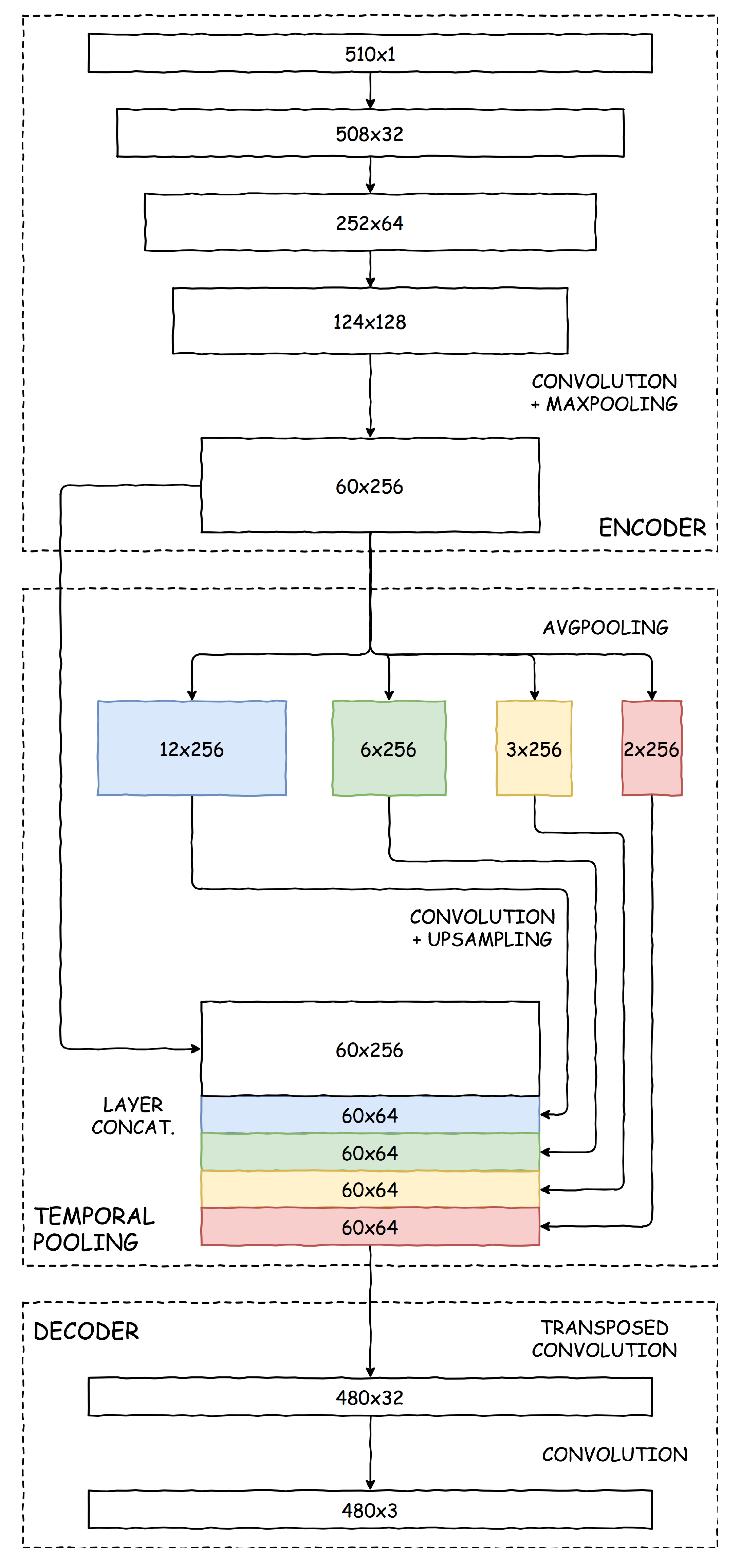
The network architecture used, which we will call Temporal Pooling NILM (TP-NILM), is an adaptation and simplification of the network called PSPNet (Pyramid Scene Parsing Network) proposed by Zhao et al. in [51] for the semantic segmentation of images. The general scheme follows the classic approach to the semantic segmentation of images, in which we have an encoder, characterised by alternating convolution and pooling modules and which allows to increase the space of the features of the signal at the cost of its temporal resolution, and a decoder module which, starting from the obtained features, reconstructs an estimate of the activation status of the equipment at the same resolution as the original signal. To these is added a module called Temporal Pooling that realizes an aggregation of the features at different resolutions, generating a form of temporal context, that embraces long periods without losing completely the resolution in the description of the signal, for the purpose of an accurate reconstruction of the activation status. The network layout is shown in the Figure 1.
The encoder is made of three convolutional filters alternated by max pooling layers, using a ReLU activation function, batch normalization downstream of the activations, and a dropout layer for regularization. The encoder reduces the time resolution of the signal by a factor of 8 and increases the signal components from a single aggregate power consumption value to 256 output features.
The temporal pooling block is used to give context information to the decoding block, creating additional features for decoding through aggregations with different resolutions of the encoder output. The encoder output passes through four average pooling modules with different filter sizes, which reduce the time resolution and keep the number of features unchanged, followed by a convolution with unit filter size, which reduces the number of features to a quarter of the input ones. The result of the convolutions constitutes the input of a ReLU activation function, followed again by batch normalization. Finally, a linear upsampling is performed to obtain a temporal resolution at the output of the temporal pooling block equal to that at the output of the encoder. A dropout is also applied to the output to regularize the network. The context features obtained from this block are linked to the detail features obtained from the encoder, doubling the overall number of features in input to the decoder.
The decoder consists of a transposed convolution layer with kernel size and stride equal to 8 that brings the temporal resolution of the signal to 1 min, while reducing the number of features. The activation function is still the ReLU. This is followed by an additional convolution layer with a unitary kernel size that maintains the time resolution and brings the number of output channels to the number of appliances being examined. A sigmoid function is used in the output and not a softmax layer as in the segmentation of the images, since while in the semantic segmentation of the images, each pixel is associated to a single class, in this case, for each time, several appliances can be simultaneously in operation.
Operating in this way, the network performs a decomposition of all appliances at the same time. This should allow, in our idea, to obtain an encoder with more general convolutive filters and not specific for a particular type of appliance and therefore to improve the ability to generalize the neural network.
The weights of the net are obtained via gradient descent optimization. The loss function is a Binary Cross-Entropy applied to each of the output channels that measures the difference between the activations estimated by the net and the actual ones for each appliance examined and for each instant of the period of time under scrutiny. The Class-Balanced Sigmoid Cross-Entropy Loss [52] has also been tested, to consider the different frequency of use of household appliances, with results worse than those obtained with the Binary Cross-Entropy. The network has been implemented using the PyTorch [53] library.
4. Experimental Setup
This section covers the numerical experiments carried out to verify the validity of the methodology proposed.
We will use the public low-frequency dataset called UK-DALE [54], which has already been extensively analysed in the literature, and for which the results obtained from different approaches are available for comparison.
4.1. Dataset
The UK-DALE dataset contains records of the power used by 5 different households in the UK. The sampling frequency of the aggregate load is 1 Hz, while the consumption of the individual appliances was recorded with a period of 6 s. The duration of the measurements and the number of activations for the appliances of interest are shown in Table 1.
The data recorded in this dataset are not uniform, neither in terms of timing nor in terms of the type of household appliance used. In our case, we will only consider the data relating to houses 1, 2 and 5. Only these dwellings have the records of the appliances we wanted to analyze in this study: refrigerator, washing machine and dishwasher. The choice of these appliances, and the exclusion of microwave ovens and kettles, for example, often discussed in the literature, is linked to the amount of energy consumption attributable to them and the possibility (for washing machines and dishwashers) to program their use in a perspective of intelligent management of consumption.
Moreover, very short consumption duration such as those of the microwave and the kettle are not well compatible with the sampling frequency chosen for the proposed methodology. The choice of this sampling frequency is linked to the type and quantity of data that it is reasonably possible to obtain from a smart meter without the use of additional energy metering systems as for our working hypothesis.
4.2. Preprocessing
The consumption data of the individual devices and the total of the houses in the dataset were pre-processed before being elaborated by the neural network. The first step was to clip the measurements of the absorbed power of the appliances to filter the measurement errors, so the maximum power was limited to the values shown in the Table 2. The time series were then sub-sampled to a period of 1 min, taking the average value of the power in the time intervals.
The activation status for individual appliances is derived from power absorption measurements in a similar way to the procedure described in [30]. A household appliance can be considered in operation when the absorbed power exceeds a certain threshold value. This criterion is sufficient to determine the state of activation of appliances operating in an ON/OFF mode, such as a fridge. When, on the other hand, the functioning of the appliance is more complex, as in the case of a dishwasher or a washing machine, the absorption can drop below the threshold value for short periods, without a washing programme having actually been completed. A minimum time is then set during which the power is maintained below the threshold value so that the appliance can be considered to be actually switched off. Finally, a minimum time is established with absorbed power above the threshold to be considered as actually switched on, in order to filter out spurious activations linked to errors in the metering.
The Table 2 shows the values used for the above-mentioned parameters for the household appliances under consideration. The values chosen are the same as those used in [30] and in the recent literature that has reviewed the same dataset.
Aggregate load data is normalized, dividing the load by a reference power value of 2000 W. The disaggregation is carried out on time windows of fixed length, with an extension of 510 samples as input and a valid output of 480 min or 8 h. The difference in size between input and output is due to the convolution filters for which no padding was used. The time series of the absorptions has been therefore divided in segments of 510 elements providing an overlay of 30 elements between successive segments so that a complete time series can be obtained by concatenating the output of the model applied to the single segments. As a last step of preprocessing, the average power absorbed in the range considered is subtracted from the signal so that the set of input values has zero average.
4.3. Postprocessing
The model returns an array of values representative of the probability of activation of each appliance for each instant being considered with a value in the range of . The activation state is estimated by evaluating the exceeding of an arbitrary threshold, chosen equal to . Moreover the same procedure of filtering of the activations used in the preprocessing stage is applied whose duration limits are the same as in the Table 2 already mentioned.
4.4. Training and Testing
Both the case (seen in the following) in which the examined dwelling is part of the training dataset (training and testing time periods are in any case strictly separated) and the case of a network trained on houses other than the one on which the test is conducted (unseen in the following) have been evaluated.
The first problem allows to evaluate the disaggregation capabilities when the signatures of the appliances in use have been measured, and the model should simply distinguish these signatures in a signal with a strong noise component due to the use of other appliances.
The second case, on the other hand, allows us to assess the model’s ability to generalise, i.e., to recognise the generic characteristics of a type of household appliance and therefore to be able to disaggregate the consumption of equipment on which no training has been conducted. The results of this case are of greater applicative interest, as they allow to estimate the performance of the algorithm in a scenario where the types of devices present in a house are known and for which only the measurement of the aggregate consumption is available.
For each house the dataset is divided into three consecutive time intervals, dedicated to training, validation and testing, which cover respectively 80%, 10% and 10% of the measurements. The split of the houses datasets for the two use cases is shown in Table 3.
For the seen case, the training is run on the first portion of the data collected for houses 1, 2 and 5, the verification is conducted on the testing portion of the data of house 1. During training, network parameters are saved whenever the target function, calculated on the data validation portion, reaches a new minimum.
In the case of unseen the training is conducted on the training portion of houses 1 and 5, the network is tested on the entire time series of house 2 and the weights of the network are saved whenever the target function, calculated on the validation portion of the data of houses 1 and 5, reaches a minimum. In summary, data from dwellings 1 and 5 are used for training and the performance check is conducted on the entire dataset of the house 2, while data from house 2 are used for performance testing only.
The network parameters are optimized with a gradient descent procedure using the Adam [55] (short for Adaptive Moment Estimation) optimization algorithm, with learning rate of , and batch size of 32. For the seen case the training lasts for 300 epochs, while the training stops at 100 epochs for the unseen case to avoid overfitting. Of course, other values have been tested both for the hyperparameters of the optimization algorithm and for the characteristics of the neural network. The values presented gave good results for the convergence times and for the accuracy obtained but do not claim to represent the combination able to guarantee the maximum accuracy for the case under examination since the aim of the work is mainly to verify the validity of the proposed approach.
Twenty different instances are trained in both cases to verify the stability of performance, and to derive the average performance of an ensemble. The number of instances of the ensemble is a reasonable compromise between the quantization of the Probability Density Function and the calculation time required.
4.5. Performance evaluation
Several metrics will be used to evaluate the performance of the proposed algorithm, aimed at capturing the effectiveness of the methodology for both the identification of the activation status and the estimation of energy consumption.
For a given instant t, indicates the activation status of a device i, unitary if on and null if off, and we indicate with the power absorbed at the same time. We denote with and the activation status and power consumption estimates obtained from the model. The accuracy of the prediction is evaluated on a time series sampled at times with .
We also define True Positive (TP), True Negative (TN), False Positive (FP) and False Negative (FN). TP refers to the number of instants of the time series in which a device is correctly identified as running, while TN is the count of instants in which the device is correctly evaluated switched off. On the contrary, FP indicates the number of instants for which an activation status is reported while the device is actually inactive, and finally FN is the count of instants in which the device is wrongly evaluated as off.
Precision in Equation (6) denotes the ratio of TPs to all instants classified as positive, while Recall in Equation (7) represents the ratio of the number of instants for which the appliance is correctly identified as operating to all instants for which the appliance is actually in function. The Accuracy defined in (5) denotes the ratio of all correctly classified instants (for both states, on or off) to all instants of the verification set. The F1 measurement defined in (8) represents the weighted average between Precision and Recall, and it is within the range of , high values indicate a better identification of the state of the appliance. Finally the Matthews Correlation Coefficient is defined in (9), whose values are in the range . A value equal to 1 denotes an exact classification, 0 denotes a random prediction while a value equal to indicates a totally wrong classification.
The accuracy of the estimate of consumption for the individual devices is measured using the Mean Absolute Error (MAE) and the Signal Aggregate Error (SAE).
where MAE is a measure of the average deviation at each instant of the estimated power with respect to the measured power, while SAE is a measure of the relative error in the estimation of the energy used during the entire evaluation period.
5. Results
The first case examined is the one called seen. The Table 4 shows the results obtained for the household appliances examined both in terms of identifying the state and in terms of estimating instantaneous and overall consumption over time.
The results are very satisfactory for all three appliances considered, as far as the identification of the activation status is concerned, in particular for the most energy consuming appliances and less for the refrigerator; the latter has a less evident signature as its maximum absorption is much lower than that of the dishwasher and washing machine. The energy performance in the strict sense is also very good, especially for the SAE metric, which identifies the overall energy consumption, with errors of around 3% of the actual value for the refrigerator and below 10% for the dishwasher and washing machine. The MAE measures the error in the instantaneous power estimation, the fact that by methodological choice the power has been modelled as constant during the whole activation period affects the maximum performance achievable on this metric.
The Table 5 shows the results obtained on the dataset for the unseen case. The performance achieved in estimating the operational status is worse than in the previous case as expected. On the contrary, the energy performances are in line with the numerical results obtained for the seen case.
The data for the dwelling not seen during the training of the network, differ from those for other houses. In house 2, in fact, there are unmonitored appliances that are different from those in other households, thus changing the characteristics of the disturbance signal present in the overall load, which is added to the consumption of the three appliances under examination. Moreover, the models of fridge, washing machine and dishwasher are different from those present in the other two houses used in the training: in terms of the power used, the length of the operating cycles and the evolution of consumption itself. In this case, the network has the difficult task of generalising the absorption of a category of household appliance and recognising its footprint in the overall consumption data.
Despite this, we can say that the performance is surprisingly good considering the limited dataset used for training, which although having a significant temporal extension, is related to a few users and therefore does not have many examples of appliances of the same class that would allow a better generalization in the training phase.
The washing machine and the dishwasher may be subject to greater differences in consumption profile, also in relation to the different washing programs available. This translates into a difficulty for the model to generalise in these cases, as mentioned above, hence the greater degradation in the classification accuracy for these two appliances compared to the refrigerator, as can be seen from the comparison of the results in Table 4 and Table 5.
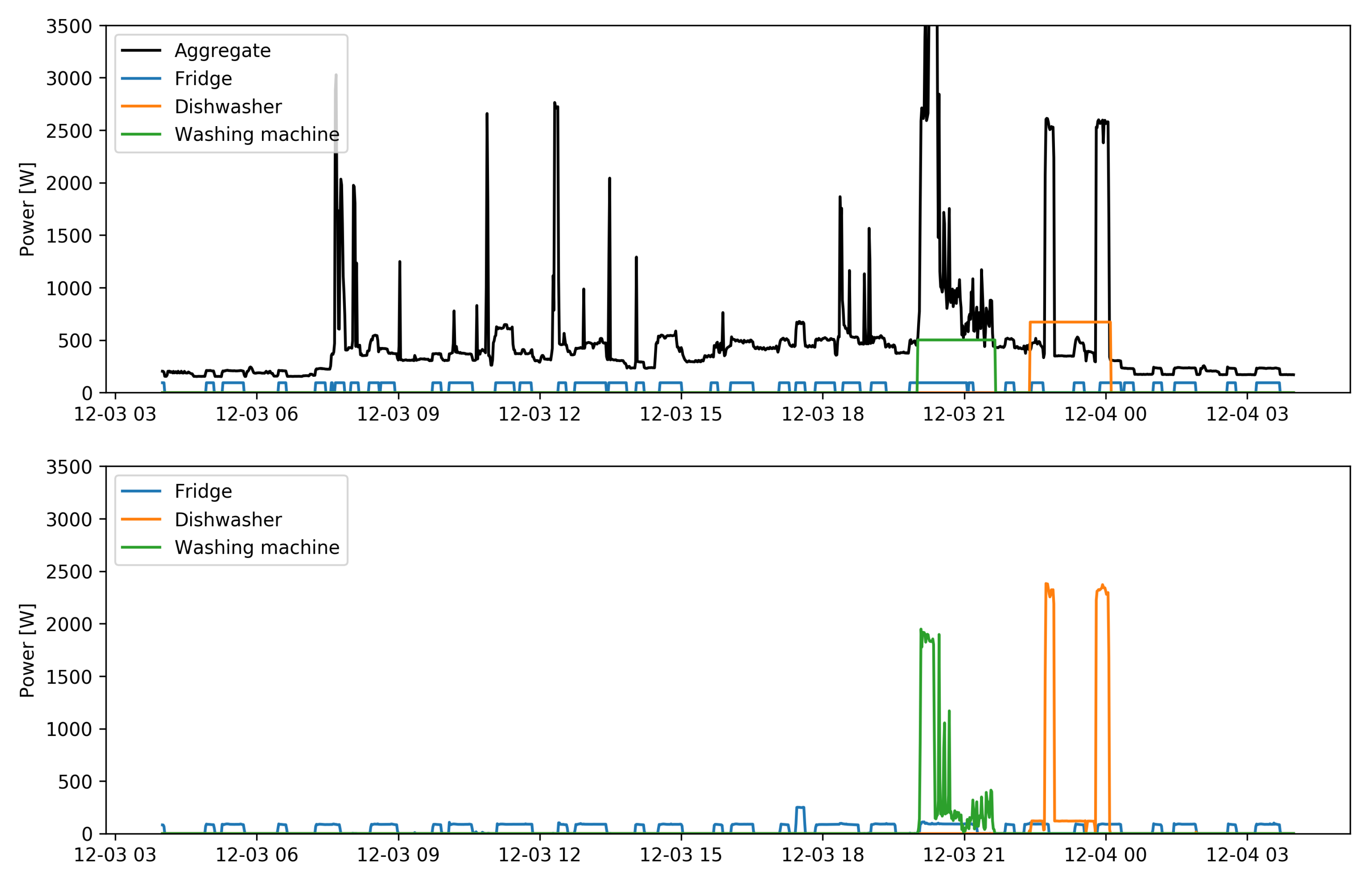
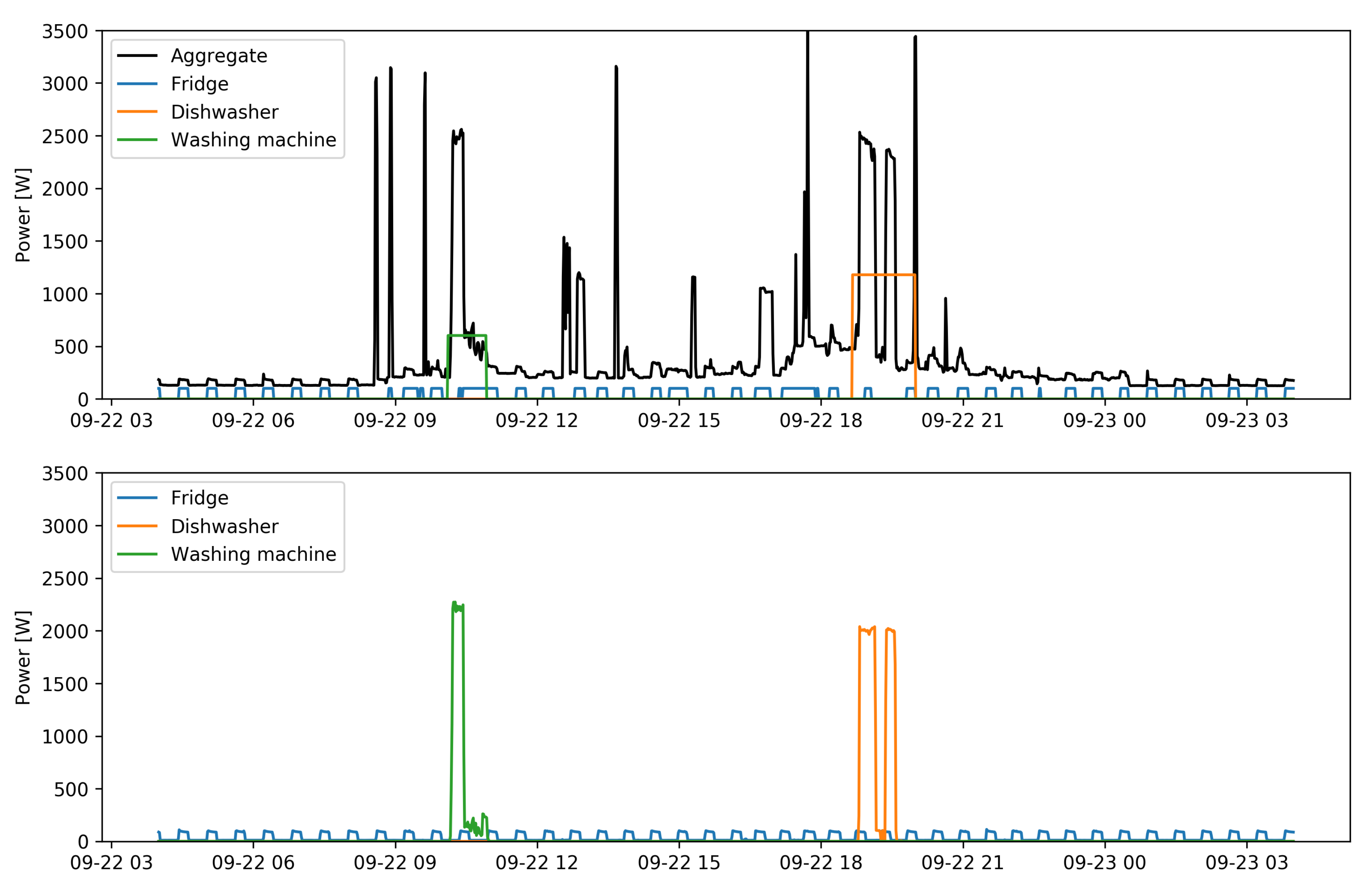
The Figure 2 and Figure 3 show an example of the results of the algorithm for a single day of data, for the seen and unseen cases respectively. In both figures the lower graph shows a day of the dataset testing portion for houses 1 and 2 respectively. The dishwasher is characterized by a period of heating of the washing water followed by a period of washing and a phase of rinsing with warm water. On the other hand, the washing machine is characterised by a water loading and heating phase followed by a washing phase in which the highly variable absorption is due to the electric motor that drives the basket. In both cases the washing cycles and the maximum absorption of the appliances (and also for the refrigerator, even if in a less evident way) are clearly different. The upper graph for the two figures shows the aggregate load and the estimated average consumption for the appliances examined.
As mentioned above, the network has been trained and tested twenty times for both the seen and the unseen cases, and in both tables are reported in addition to the mean value of the ensemble of the results obtained from the 20 models also the intervals of variation of the results obtained for the individual instances. The scores are more stable for the Table 4, highlighting the need for training conducted on a larger number of users, in order to further improve the performance of the algorithm.
6. Discussion
The use of a public dataset allows to evaluate the results obtained in comparison with other methodologies published in the literature. Unfortunately, not all of the published studies address both proposed cases, the seen case, in which training and verification are conducted on the same home, and the unseen case, in which verification is conducted on a different user than the one on which the network has been trained.
The Table 6 shows the comparison of the performance of our model (TP-NILM) with the models in the literature for the seen case.
The TP-NILM model offers good performances as far as the recognition of the state of activation is concerned, also the accuracy in the estimate of the total consumptions (SAE) is satisfactory, while the value of the MAE is affected by the assumption made about the constancy of the consumption for each cycle of activation. The best performance is obtained for high-consumption appliances, while the algorithm we have proposed seems to have more difficulty in correctly identifying the activations of the fridge. In this regard, it is worth remembering that we intentionally under-sampled the time series. In the case of the refrigerator, the maximum power absorbed is much lower than that of a dishwasher or washing machine so that the periodic activations can easily be confused with the noise associated with the many other unmonitored loads that contribute to the overall aggregate load. The absorption of the refrigerator, however, is characterized by the activation of a marked absorption linked to the starting point of the compressor, lasting less than a minute, which can only be detected by the original sampling of the dataset.
Furthermore, it is necessary to specify a detail that is relevant to the practical importance of these services. With the exception of the method described in [48], all other methods require knowledge of the consumption of individual equipment throughout the training period for a given user. The application of these methods therefore requires the installation of measuring devices for individual household appliances, and that these have been recording energy consumption throughout the training period. It is therefore debatable to define the application of these methods to the same user as Non-intrusive Load Monitoring. In the procedure proposed we use only information relating to the status of activation of the same equipment that can be acquired independently of the reading of consumption, in automatic or semi-automatic mode through interaction with the user.
The unseen case is certainly more interesting, where the model is applied to a user whose only known time series is the aggregate load, as well as the type and nominal consumption of the appliances to be monitored. The performances obtained with our method are compared with the values published in the literature on the same dataset in the Table 7.
The procedure is effective both in estimating the state of activation and in energy metrics, obtaining good results when compared with other methods, especially for the dishwasher and washing machine. In general the performance, for each of the methods considered, is worse than in the seen case, demonstrating on the one hand the difficulty of obtaining generic models, and on the other hand the obvious added value of a specific modeling for a given dwelling. In particular, the Deep AE method obtains better performances for the fridge, similar performances for the dishwasher but surprisingly worse for the washing machine, in our opinion due to the marked difference in the consumption curve of this appliance for each of the three houses. Probably the Deep AE method, based on a technique of the Auto Encoder type, does not have the same generalizing capabilities of the method we proposed, which we think derive from the features pooling module at different time scales. Other methods also based on an Autoencoder approach such as seq2seq and seq2point have comparable performance in terms of MAE but unfortunately their accuracy is not declared for the recognition of the activation state. The results of the unseen case are also interesting given the limited number of different appliances on which it was possible to carry out the training, as richer datasets could lead to even better generalization.
7. Conclusions
In this paper we have presented a new methodology for Non Intrusive Load Monitoring and Disaggregation, based on the recognition of the activation states of household appliances. The approach is based on the observation that a sufficiently experienced user is capable of recognizing these activation states by examining an aggregate consumption plot and that a neural network like the one proposed can emulate that ability. Leveraging the latest techniques used for semantic image segmentation, we have introduced a model based on convolutional networks, applicable on datasets with low sampling rate. The space of the features used for the classification has been enriched through the introduction of a temporal pooling module that performs a pooling at different time scales of the features calculated in the first convolution levels, thus increasing the receptive field without compromising the temporal resolution of the output. The approach is based on the multilabel classification of simultaneous active loads, and estimates the consumption of appliances as a constant average value during activation. This approach allows us to obtain good generalization characteristics for the algorithm, allowing the application of a trained network to a household not used for the training with good performance on a reference dataset.
In this work, the disaggregation was carried out by examining the time series of the active power consumed only, but additional variables can be considered. If available, the reactive power data could improve the performance, but also information on the time of use, or the environmental temperature conditions are additional features that could improve the performance of the algorithm. In fact, from the analysis of the time series of dishwashers and washing machines, one can notice habits of use, for example the dishwasher is activated in the evening hours, after dinner; the environmental conditions, on the other hand, can influence the refrigerator and certainly the heating systems not considered in this work.
A further line of research is the realization of an active learning procedure for the optimization of performance on a given user using a reduced feedback from a pre-trained network on users other than the one examined.
Author Contributions
L.M., M.M. and S.M. jointly conceived and designed the methodologies, performed the analysis and wrote the paper. All authors have read and agreed to the published version of the manuscript.
Funding
This research was funded by Regione Autonoma della Sardegna, Delibera 66/14 del 13.12.2016, Progetto Complesso area ICT.
Conflicts of Interest
The authors declare no conflict of interest.
References
- Wittmann, F.M.; López, J.C.; Rider, M.J. Nonintrusive load monitoring algorithm using mixed-integer linear programming. IEEE Trans. Consum. Electron. 2018, 64, 180–187. [Google Scholar] [CrossRef]
- Armel, K.C.; Gupta, A.; Shrimali, G.; Albert, A. Is disaggregation the holy grail of energy efficiency? The case of electricity. Energy Policy 2013, 52, 213–234. [Google Scholar] [CrossRef] [Green Version]
- Al-Ali, A.R.; Zualkernan, I.A.; Rashid, M.; Gupta, R.; Alikarar, M. A smart home energy management system using IoT and big data analytics approach. IEEE Trans. Consum. Electron. 2017, 63, 426–434. [Google Scholar] [CrossRef]
- Han, D.M.; Lim, J.H. Smart home energy management system using IEEE 802.15. 4 and zigbee. IEEE Trans. Consum. Electron. 2010, 56, 1403–1410. [Google Scholar] [CrossRef]
- Esa, N.F.; Abdullah, M.P.; Hassan, M.Y. A review disaggregation method in Non-intrusive Appliance Load Monitoring. Renew. Sustain. Energy Rev. 2016, 66, 163–173. [Google Scholar] [CrossRef]
- Hosseini, S.S.; Agbossou, K.; Kelouwani, S.; Cardenas, A. Non-intrusive load monitoring through home energy management systems: A comprehensive review. Renew. Sustain. Energy Rev. 2017, 79, 1266–1274. [Google Scholar] [CrossRef]
- Wang, Y.; Chen, Q.; Hong, T.; Kang, C. Review of smart meter data analytics: Applications, methodologies, and challenges. IEEE Trans. Smart Grid 2018, 10, 3125–3148. [Google Scholar] [CrossRef] [Green Version]
- Ruano, A.; Hernandez, A.; Ureña, J.; Ruano, M.; Garcia, J. NILM techniques for intelligent home energy management and ambient assisted living: A review. Energies 2019, 12, 2203. [Google Scholar] [CrossRef] [Green Version]
- Figueiredo, M.; Ribeiro, B.; de Almeida, A. Analysis of trends in seasonal electrical energy consumption via non-negative tensor factorization. Neurocomputing 2015, 170, 318–327. [Google Scholar] [CrossRef] [Green Version]
- Makonin, S.W. Real-Time Embedded Low-Frequency Load Disaggregation. Ph.D. Thesis, Applied Sciences: School of Computing Science, Simon Fraser University, Burnaby, BC, Canada, 2014. [Google Scholar]
- Lu-Lulu, L.L.; Park, S.W.; Wang, B.H. Electric load signature analysis for home energy monitoring system. Int. J. Fuzzy Logic Intell. Syst. 2012, 12, 193–197. [Google Scholar] [CrossRef] [Green Version]
- Elhamifar, E.; Sastry, S. Energy Disaggregation via Learning Powerlets and Sparse Coding; AAAI: Menlo Park, CA, USA, 2015; pp. 629–635. [Google Scholar]
- Hasan, M.; Chowdhury, D.; Khan, M.; Rahman, Z. Non-Intrusive Load Monitoring Using Current Shapelets. Appl. Sci. 2019, 9, 5363. [Google Scholar] [CrossRef] [Green Version]
- Du, L.; Yang, Y.; He, D.; Harley, R.G.; Habetler, T.G. Feature extraction for load identification using long-term operating waveforms. IEEE Trans. Smart Grid 2014, 6, 819–826. [Google Scholar] [CrossRef]
- Meehan, P.; McArdle, C.; Daniels, S. An efficient, scalable time-frequency method for tracking energy usage of domestic appliances using a two-step classification algorithm. Energies 2014, 7, 7041–7066. [Google Scholar] [CrossRef] [Green Version]
- Chang, H.H.; Lian, K.L.; Su, Y.C.; Lee, W.J. Power-spectrum-based wavelet transform for nonintrusive demand monitoring and load identification. IEEE Trans. Ind. Appl. 2013, 50, 2081–2089. [Google Scholar] [CrossRef]
- Lin, Y.H.; Tsai, M.S. Development of an improved time–frequency analysis-based nonintrusive load monitor for load demand identification. IEEE Trans. Instrum. Meas. 2013, 63, 1470–1483. [Google Scholar] [CrossRef]
- Hassan, T.; Javed, F.; Arshad, N. An empirical investigation of VI trajectory based load signatures for non-intrusive load monitoring. IEEE Trans. Smart Grid 2013, 5, 870–878. [Google Scholar] [CrossRef] [Green Version]
- Wang, A.L.; Chen, B.X.; Wang, C.G.; Hua, D. Non-intrusive load monitoring algorithm based on features of V–I trajectory. Electr. Power Syst. Res. 2018, 157, 134–144. [Google Scholar] [CrossRef]
- Bouhouras, A.S.; Gkaidatzis, P.A.; Chatzisavvas, K.C.; Panagiotou, E.; Poulakis, N.; Christoforidis, G.C. Load signature formulation for non-intrusive load monitoring based on current measurements. Energies 2017, 10, 538. [Google Scholar] [CrossRef]
- Bouhouras, A.S.; Gkaidatzis, P.A.; Panagiotou, E.; Poulakis, N.; Christoforidis, G.C. A NILM algorithm with enhanced disaggregation scheme under harmonic current vectors. Energy Build. 2019, 183, 392–407. [Google Scholar] [CrossRef]
- Piga, D.; Cominola, A.; Giuliani, M.; Castelletti, A.; Rizzoli, A.E. Sparse optimization for automated energy end use disaggregation. IEEE Trans. Control Syst. Technol. 2015, 24, 1044–1051. [Google Scholar] [CrossRef]
- Wang, H.; Yang, W. An iterative load disaggregation approach based on appliance consumption pattern. Appl. Sci. 2018, 8, 542. [Google Scholar] [CrossRef] [Green Version]
- Wytock, M.; Kolter, J.Z. Contextually supervised source separation with application to energy disaggregation. In Proceedings of the Twenty-Eighth AAAI Conference on Artificial Intelligence, Québec City, QC, Canada, 27–31 July 2014. [Google Scholar]
- Kong, W.; Dong, Z.Y.; Hill, D.J.; Luo, F.; Xu, Y. Improving nonintrusive load monitoring efficiency via a hybrid programing method. IEEE Trans. Ind. Inform. 2016, 12, 2148–2157. [Google Scholar] [CrossRef]
- Kong, W.; Dong, Z.Y.; Ma, J.; Hill, D.J.; Zhao, J.; Luo, F. An extensible approach for non-intrusive load disaggregation with smart meter data. IEEE Trans. Smart Grid 2016, 9, 3362–3372. [Google Scholar] [CrossRef]
- Egarter, D.; Sobe, A.; Elmenreich, W. Evolving non-intrusive load monitoring. In Proceedings of the European Conference on the Applications of Evolutionary Computation, Vienna, Austria, 3–5 April 2013; Springer: Berlin/Heidelberg, Germany, 2013; pp. 182–191. [Google Scholar]
- Lucas, A.; Jansen, L.; Andreadou, N.; Kotsakis, E.; Masera, M. Load Flexibility Forecast for DR Using Non-Intrusive Load Monitoring in the Residential Sector. Energies 2019, 12, 2725. [Google Scholar] [CrossRef] [Green Version]
- Chang, H.H. Non-intrusive demand monitoring and load identification for energy management systems based on transient feature analyses. Energies 2012, 5, 4569–4589. [Google Scholar] [CrossRef] [Green Version]
- Kelly, J.; Knottenbelt, W. Neural NILM: Deep neural networks applied to energy disaggregation. In Proceedings of the 2nd ACM International Conference on Embedded Systems for Energy-Efficient Built Environments, Bengaluru, India, 4–8 January 2015; ACM: New York, NY, USA, 2015; pp. 55–64. [Google Scholar]
- Zhang, C.; Zhong, M.; Wang, Z.; Goddard, N.; Sutton, C. Sequence-to-point learning with neural networks for non-intrusive load monitoring. In Proceedings of the Thirty-Second AAAI Conference on Artificial Intelligence, New Orleans, LA, USA, 2–7 February 2018; pp. 2604–2611. [Google Scholar]
- Bonfigli, R.; Felicetti, A.; Principi, E.; Fagiani, M.; Squartini, S.; Piazza, F. Denoising autoencoders for non-intrusive load monitoring: Improvements and comparative evaluation. Energy Build. 2018, 158, 1461–1474. [Google Scholar] [CrossRef]
- Barsim, K.S.; Yang, B. On the feasibility of generic deep disaggregation for single-load extraction. arXiv 2018, arXiv:1802.02139. [Google Scholar]
- Fagiani, M.; Bonfigli, R.; Principi, E.; Squartini, S.; Mandolini, L. A Non-Intrusive Load Monitoring Algorithm Based on Non-Uniform Sampling of Power Data and Deep Neural Networks. Energies 2019, 12, 1371. [Google Scholar] [CrossRef] [Green Version]
- Xia, M.; Wang, K.; Zhang, X.; Xu, Y. Non-intrusive load disaggregation based on deep dilated residual network. Electr. Power Syst. Res. 2019, 170, 277–285. [Google Scholar] [CrossRef]
- Wu, Q.; Wang, F. Concatenate convolutional neural networks for non-intrusive load monitoring across complex background. Energies 2019, 12, 1572. [Google Scholar] [CrossRef] [Green Version]
- Mauch, L.; Yang, B. A new approach for supervised power disaggregation by using a deep recurrent LSTM network. In Proceedings of the 2015 IEEE Global Conference on Signal and Information Processing (GlobalSIP), Orlando, FL, USA, 14–16 December 2015; IEEE: Piscataway, NJ, USA, 2015; pp. 63–67. [Google Scholar]
- Rafiq, H.; Zhang, H.; Li, H.; Ochani, M.K. Regularized LSTM Based Deep Learning Model: First Step towards Real-Time Non-Intrusive Load Monitoring. In Proceedings of the 2018 IEEE International Conference on Smart Energy Grid Engineering (SEGE), Oshawa, ON, Canada, 12–15 August 2018; IEEE: Piscataway, NJ, USA, 2018; pp. 234–239. [Google Scholar]
- Kim, J.G.; Lee, B. Appliance classification by power signal analysis based on multi-feature combination multi-layer LSTM. Energies 2019, 12, 2804. [Google Scholar] [CrossRef] [Green Version]
- Salerno, V.M.; Rabbeni, G. An extreme learning machine approach to effective energy disaggregation. Electronics 2018, 7, 235. [Google Scholar] [CrossRef] [Green Version]
- Kramer, O.; Wilken, O.; Beenken, P.; Hein, A.; Hüwel, A.; Klingenberg, T.; Meinecke, C.; Raabe, T.; Sonnenschein, M. On ensemble classifiers for nonintrusive appliance load monitoring. In Proceedings of the International Conference on Hybrid Artificial Intelligence Systems, Hong Kong, China, 4–7 December 2012; pp. 322–331. [Google Scholar]
- Figueiredo, M.B.; De Almeida, A.; Ribeiro, B. An experimental study on electrical signature identification of non-intrusive load monitoring (nilm) systems. In Proceedings of the International Conference on Adaptive and Natural Computing Algorithms, Ljubljana, Slovenia, 14–16 April 2011; pp. 31–40. [Google Scholar]
- Wu, X.; Gao, Y.; Jiao, D. Multi-label classification based on random forest algorithm for non-intrusive load monitoring system. Processes 2019, 7, 337. [Google Scholar] [CrossRef] [Green Version]
- He, H.; Liu, Z.; Jiao, R.; Yan, G. A novel nonintrusive load monitoring approach based on linear-chain conditional random fields. Energies 2019, 12, 1797. [Google Scholar] [CrossRef] [Green Version]
- Agyeman, K.A.; Han, S.; Han, S. Real-time recognition non-intrusive electrical appliance monitoring algorithm for a residential building energy management system. Energies 2015, 8, 9029–9048. [Google Scholar] [CrossRef]
- Cominola, A.; Giuliani, M.; Piga, D.; Castelletti, A.; Rizzoli, A.E. A hybrid signature-based iterative disaggregation algorithm for non-intrusive load monitoring. Appl. Energy 2017, 185, 331–344. [Google Scholar] [CrossRef]
- Makonin, S.; Popowich, F.; Bajić, I.V.; Gill, B.; Bartram, L. Exploiting HMM sparsity to perform online real-time nonintrusive load monitoring. IEEE Trans. Smart Grid 2016, 7, 2575–2585. [Google Scholar] [CrossRef]
- Mengistu, M.A.; Girmay, A.A.; Camarda, C.; Acquaviva, A.; Patti, E. A cloud-based on-line disaggregation algorithm for home appliance loads. IEEE Trans. Smart Grid 2018, 10, 3430–3439. [Google Scholar] [CrossRef]
- Desai, S.; Alhadad, R.; Mahmood, A.; Chilamkurti, N.; Rho, S. Multi-State Energy Classifier to Evaluate the Performance of the NILM Algorithm. Sensors 2019, 19, 5236. [Google Scholar] [CrossRef] [Green Version]
- Yu, J.; Gao, Y.; Wu, Y.; Jiao, D.; Su, C.; Wu, X. Non-Intrusive Load Disaggregation by Linear Classifier Group Considering Multi-Feature Integration. Appl. Sci. 2019, 9, 3558. [Google Scholar] [CrossRef] [Green Version]
- Zhao, H.; Shi, J.; Qi, X.; Wang, X.; Jia, J. Pyramid scene parsing network. In Proceedings of the IEEE Conference on Computer Vision and Pattern Recognition, Honolulu, HI, USA, 21–26 July 2017; pp. 2881–2890. [Google Scholar]
- Cui, Y.; Jia, M.; Lin, T.Y.; Song, Y.; Belongie, S. Class-Balanced Loss Based on Effective Number of Samples. In Proceedings of the IEEE Conference on Computer Vision and Pattern Recognition (CVPR), Long Beach, CA, USA, 16–20 June 2019. [Google Scholar]
- Paszke, A.; Gross, S.; Chintala, S.; Chanan, G.; Yang, E.; DeVito, Z.; Lin, Z.; Desmaison, A.; Antiga, L.; Lerer, A. Automatic Differentiation in PyTorch. In Proceedings of the NIPS Autodiff Workshop, Long Beach, CA, USA, 8 December 2017. [Google Scholar]
- Kelly, J.; Knottenbelt, W. The UK-DALE dataset, domestic appliance-level electricity demand and whole-house demand from five UK homes. Sci. Data 2015, 2, 150007. [Google Scholar] [CrossRef] [PubMed] [Green Version]
- Kingma, D.P.; Ba, J. Adam: A method for stochastic optimization. arXiv 2014, arXiv:1412.6980. [Google Scholar]
Figure 1.
Outline of the network architecture used. See text in Section 3 for details.
Figure 1.
Outline of the network architecture used. See text in Section 3 for details.

Figure 2.
Example of load disaggregation for the seen case. The upper graph shows the aggregate load and the estimated consumption obtained by the method, while the lower graph shows true values of the power absorbed by the three appliances. The estimated value of the consumption of household appliances in the upper part of the figure is assumed to be constant for the activation periods and equal to the average consumption during use.

Figure 3.
Example of load disaggregation for the unseen case. The upper graph shows the aggregate load and the estimated consumption obtained by the method, while the lower graph shows true values of the power absorbed by the three appliances. The estimated value of the consumption of household appliances in the upper part of the figure is assumed to be constant for the activation periods and equal to the average consumption during use.


Table 1.
Duration of measurements and number of appliance activations in UK-DALE dataset houses.
| House 1 | House 2 | House 3 | House 4 | House 5 | |
|---|---|---|---|---|---|
| Duration (days) | 612 | 134 | 33 | 199 | 64 |
| Fridge activations (-) | 16,240 | 3525 | 20 | 4682 | 1489 |
| Dishwasher activations (-) | 197 | 98 | 0 | 0 | 23 |
| Washing machine activations (-) | 513 | 54 | 0 | 0 | 55 |
Table 2.
Parameters used to derive the activation status of household appliances from measurements of the absorbed power.
Table 2.
Parameters used to derive the activation status of household appliances from measurements of the absorbed power.
| Fridge | Dishwasher | Washing Machine | |
|---|---|---|---|
| Max. power (W) | 300 | 2500 | 2500 |
| Power threshold (W) | 50 | 10 | 20 |
| OFF duration (min) | 0 | 3 | 30 |
| ON duration (min) | 1 | 30 | 30 |
Table 3.
Training, Validation and Testing dataset composition for the seen and unseen use cases.
| Use Case: seen | Use Case: unseen | |||||
|---|---|---|---|---|---|---|
| Training (%) | Validation (%) | Testing (%) | Training (%) | Validation (%) | Testing (%) | |
| House 1 | 80 | 10 | 10 | 80 | 10 | - |
| House 2 | 80 | - | - | - | - | 100 |
| House 5 | 80 | - | - | 80 | 10 | - |
Table 4.
Performance of the method for the seen case for house 1 of the UK-DALE dataset. 20 different instances of the neural network have been trained and the value of the ensemble estimate and the 90% range of performance variation are reported.
Table 4.
Performance of the method for the seen case for house 1 of the UK-DALE dataset. 20 different instances of the neural network have been trained and the value of the ensemble estimate and the 90% range of performance variation are reported.
| Fridge | Dishwasher | Washing Machine | ||||
|---|---|---|---|---|---|---|
| Ensemble Mean | 90% Interval | Ensemble Mean | 90% Interval | Ensemble Mean | 90% Interval | |
| Precision | 0.875 | (0.867, 0.885) | 0.942 | (0.904, 0.966) | 0.975 | (0.968, 0.979) |
| Recall | 0.859 | (0.846, 0.871) | 0.919 | (0.890, 0.942) | 0.982 | (0.977, 0.987) |
| Accuracy | 0.880 | (0.878, 0.882) | 0.997 | (0.995, 0.997) | 0.997 | (0.996, 0.997) |
| F1 score | 0.867 | (0.864, 0.870) | 0.930 | (0.905, 0.946) | 0.978 | (0.976, 0.980) |
| MCC | 0.759 | (0.755, 0.762) | 0.928 | (0.903, 0.945) | 0.977 | (0.974, 0.979) |
| MAE [W] | 15.25 | (15.08, 15.47) | 20.41 | (19.99, 21.00) | 41.97 | (41.80, 42.21) |
| SAE | −0.020 | (−0.046, 0.002) | −0.042 | (−0.082, −0.005) | −0.077 | (−0.085, −0.066) |
Table 5.
Performance of the method for the unseen case for house 2 of the UK-DALE dataset. In total, 20 different instances of the neural network have been trained and the value of the ensemble estimate and the 90% range of performance variation are reported.
Table 5.
Performance of the method for the unseen case for house 2 of the UK-DALE dataset. In total, 20 different instances of the neural network have been trained and the value of the ensemble estimate and the 90% range of performance variation are reported.
| Fridge | Dishwasher | Washing Machine | ||||
|---|---|---|---|---|---|---|
| Ensemble Mean | 90% Interval | Ensemble Mean | 90% Interval | Ensemble Mean | 90% Interval | |
| Precision | 0.892 | (0.883, 0.898) | 0.788 | (0.738, 0.826) | 0.858 | (0.811, 0.893) |
| Recall | 0.851 | (0.841, 0.861) | 0.835 | (0.768, 0.897) | 0.869 | (0.827, 0.918) |
| Accuracy | 0.905 | (0.900, 0.908) | 0.989 | (0.987, 0.990) | 0.997 | (0.996, 0.998) |
| F1 score | 0.871 | (0.863, 0.876) | 0.809 | (0.790, 0.822) | 0.863 | (0.835, 0.900) |
| MCC | 0.796 | (0.786, 0.803) | 0.805 | (0.784, 0.817) | 0.862 | (0.834, 0.899) |
| MAE [W] | 17.03 | (16.82, 17.24) | 33.07 | (31.19, 35.68) | 8.31 | (7.88, 8.70) |
| SAE | −0.046 | (−0.066, −0.025) | 0.063 | (−0.054, 0.219) | 0.014 | (−0.059, 0.115) |
Table 6.
Performance comparison for the seen case on the UK-DALE dataset. The models used for comparison are based on Combinatorial Optimization (Neural-NILM CO), Hidden Markov Model (Neural-NILM FHMM, ON-line-NILM), Convolutional Neural Network (Neural-NILM AE, Neural-NILM Rect., dAE, Deep AE, D-ResNet), Recurrent Neural Networks (Neural-NILM LSTM) and Extreme Learning Machine (H-ELM).
| Fridge | |||||||
| Prec. | Rec. | Acc. | F1 | MCC | MAE | SAE | |
| Neural-NILM CO [30] | 0.50 | 0.54 | 0.61 | 0.52 | - | 50 | 0.26 |
| Neural-NILM FHMM [30] | 0.39 | 0.63 | 0.46 | 0.47 | - | 69 | 0.50 |
| Neural-NILM AE [30] | 0.83 | 0.79 | 0.85 | 0.81 | - | 25 | −0.35 |
| Neural-NILM Rect. [30] | 0.71 | 0.77 | 0.79 | 0.74 | - | 22 | −0.07 |
| Neural-NILM LSTM [30] | 0.71 | 0.67 | 0.76 | 0.69 | - | 34 | −0.22 |
| dAE [32] | - | - | - | 0.78 | 0.68 | - | - |
| Deep AE [33] | - | - | - | 0.88 | - | - | - |
| On-line-NILM [48] | 0.73 | 0.87 | 0.82 | 0.79 | - | 4.34 | - |
| H-ELM [40] | 0.88 | 0.80 | 0.88 | 0.89 | - | 20 | - |
| D-ResNet [35] | 1.00 | 0.99 | 1.00 | 0.99 | - | 2.63 | 0.02 |
| TP-NILM | 0.88 | 0.86 | 0.88 | 0.87 | 0.76 | 15.25 | −0.02 |
| Dishwasher | |||||||
| Prec. | Rec. | Acc. | F1 | MCC | MAE | SAE | |
| Neural-NILM CO [30] | 0.07 | 0.50 | 0.69 | 0.11 | - | 75 | 0.28 |
| Neural-NILM FHMM [30] | 0.04 | 0.78 | 0.37 | 0.08 | - | 111 | 0.66 |
| Neural-NILM AE [30] | 0.45 | 0.99 | 0.95 | 0.60 | - | 21 | −0.34 |
| Neural-NILM Rect. [30] | 0.88 | 0.61 | 0.98 | 0.72 | - | 30 | −0.53 |
| Neural-NILM LSTM [30] | 0.03 | 0.63 | 0.35 | 0.06 | - | 130 | 0.76 |
| dAE [32] | - | - | - | 0.56 | 0.58 | - | - |
| Deep AE [33] | - | - | - | 0.80 | - | - | - |
| On-line-NILM [48] | 0.78 | 0.44 | 0.71 | 0.56 | - | 27.72 | - |
| H-ELM [40] | 0.89 | 0.99 | 0.98 | 0.75 | - | 19 | - |
| D-ResNet [35] | 0.78 | 0.81 | 0.99 | 0.80 | - | 7.80 | 0.01 |
| TP-NILM | 0.94 | 0.92 | 1.00 | 0.93 | 0.93 | 20.41 | −0.04 |
| Washing machine | |||||||
| Prec. | Rec. | Acc. | F1 | MCC | MAE | SAE | |
| Neural-NILM CO [30] | 0.08 | 0.56 | 0.69 | 0.13 | - | 88 | 0.65 |
| Neural-NILM FHMM [30] | 0.06 | 0.87 | 0.39 | 0.11 | - | 138 | 0.76 |
| Neural-NILM AE [30] | 0.15 | 0.99 | 0.76 | 0.25 | - | 44 | 0.18 |
| Neural-NILM Rect. [30] | 0.72 | 0.38 | 0.97 | 0.49 | - | 28 | −0.65 |
| Neural-NILM LSTM [30] | 0.05 | 0.62 | 0.31 | 0.09 | - | 133 | 0.73 |
| dAE [32] | - | - | - | 0.41 | 0.43 | - | - |
| Deep AE [33] | - | - | - | 0.96 | - | - | - |
| On-line-NILM [48] | 0.60 | 1.00 | 0.60 | 0.70 | - | 118.11 | - |
| H-ELM [40] | 0.73 | 0.99 | 0.76 | 0.50 | - | 27 | - |
| D-ResNet [35] | 0.93 | 0.75 | 1.00 | 0.83 | - | 2.97 | 0.07 |
| TP-NILM | 0.98 | 0.98 | 1.00 | 0.98 | 0.98 | 41.97 | −0.08 |
Table 7.
Performance comparison for the unseen case on the UK-DALE dataset. The models used for comparison are based on Combinatorial Optimization (Neural-NILM CO), Hidden Markov Model (Neural-NILM FHMM, ON-line-NILM), Convolutional Neural Network (Neural-NILM AE, Neural-NILM Rect., dAE, seq2seq, seq2point, Deep AE), Recurrent Neural Networks (Neural-NILM LSTM) and Extreme Learning Machine (H-ELM).
| Fridge | |||||||
| Prec. | Rec. | Acc. | F1 | MCC | MAE | SAE | |
| Neural-NILM CO [30] | 0.30 | 0.41 | 0.45 | 0.35 | - | 73 | 0.37 |
| Neural-NILM FHMM [30] | 0.40 | 0.86 | 0.50 | 0.55 | - | 67 | 0.57 |
| Neural-NILM AE [30] | 0.85 | 0.88 | 0.90 | 0.87 | - | 26 | −0.38 |
| Neural-NILM Rect. [30] | 0.79 | 0.86 | 0.87 | 0.82 | - | 18 | −0.13 |
| Neural-NILM LSTM [30] | 0.72 | 0.77 | 0.81 | 0.74 | - | 36 | −0.25 |
| dAE [32] | - | - | - | 0.83 | 0.76 | - | - |
| seq2seq [31] | - | - | - | - | - | 24.5 | 0.37 |
| seq2point [31] | - | - | - | - | - | 20.9 | 0.12 |
| H-ELM [40] | 0.90 | 0.92 | 0.94 | 0.89 | - | 23 | - |
| Deep AE [33] | - | - | - | 0.93 | - | - | - |
| TP-NILM | 0.89 | 0.85 | 0.91 | 0.87 | 0.80 | 17.03 | −0.05 |
| Dishwasher | |||||||
| Prec. | Rec. | Acc. | F1 | MCC | MAE | SAE | |
| Neural-NILM CO [30] | 0.06 | 0.67 | 0.64 | 0.11 | - | 74 | 0.62 |
| Neural-NILM FHMM [30] | 0.03 | 0.49 | 0.33 | 0.05 | - | 110 | 0.75 |
| Neural-NILM AE [30] | 0.29 | 0.99 | 0.92 | 0.44 | - | 24 | −0.33 |
| Neural-NILM Rect. [30] | 0.89 | 0.64 | 0.99 | 0.74 | - | 30 | −0.31 |
| Neural-NILM LSTM [30] | 0.04 | 0.87 | 0.30 | 0.08 | - | 168 | 0.87 |
| dAE [32] | - | - | - | 0.51 | 0.50 | - | - |
| seq2seq [31] | - | - | - | - | - | 32.5 | 0.78 |
| seq2point [31] | - | - | - | - | - | 27.7 | 0.65 |
| H-ELM [40] | 0.35 | 1.00 | 1.00 | 0.55 | - | 22 | - |
| Deep AE [33] | - | - | - | 0.80 | - | - | - |
| TP-NILM | 0.79 | 0.84 | 0.99 | 0.81 | 0.81 | 33.07 | 0.06 |
| Washing machine | |||||||
| Prec. | Rec. | Acc. | F1 | MCC | MAE | SAE | |
| Neural-NILM CO [30] | 0.06 | 0.48 | 0.88 | 0.10 | - | 39 | 0.73 |
| Neural-NILM FHMM [30] | 0.04 | 0.64 | 0.79 | 0.08 | - | 67 | 0.86 |
| Neural-NILM AE [30] | 0.07 | 1.00 | 0.82 | 0.13 | - | 24 | 0.48 |
| Neural-NILM Rect. [30] | 0.29 | 0.24 | 0.98 | 0.27 | - | 11 | −0.74 |
| Neural-NILM LSTM [30] | 0.01 | 0.73 | 0.23 | 0.03 | - | 109 | 0.91 |
| dAE [32] | - | - | - | 0.68 | 0.69 | - | - |
| seq2seq [31] | - | - | - | - | - | 10.1 | 0.45 |
| seq2point [31] | - | - | - | - | - | 12.7 | 0.28 |
| H-ELM [40] | 0.10 | 1.00 | 0.84 | 0.43 | - | 21 | - |
| Deep AE [33] | - | - | - | 0.41 | - | - | - |
| TP-NILM | 0.86 | 0.87 | 1.00 | 0.86 | 0.86 | 8.31 | 0.01 |
© 2020 by the authors. Licensee MDPI, Basel, Switzerland. This article is an open access article distributed under the terms and conditions of the Creative Commons Attribution (CC BY) license (http://creativecommons.org/licenses/by/4.0/).
Share and Cite
MDPI and ACS Style
Massidda, L.; Marrocu, M.; Manca, S. Non-Intrusive Load Disaggregation by Convolutional Neural Network and Multilabel Classification. Appl. Sci. 2020, 10, 1454. https://0-doi-org.brum.beds.ac.uk/10.3390/app10041454
AMA Style
Massidda L, Marrocu M, Manca S. Non-Intrusive Load Disaggregation by Convolutional Neural Network and Multilabel Classification. Applied Sciences. 2020; 10(4):1454. https://0-doi-org.brum.beds.ac.uk/10.3390/app10041454
Chicago/Turabian StyleMassidda, Luca, Marino Marrocu, and Simone Manca. 2020. "Non-Intrusive Load Disaggregation by Convolutional Neural Network and Multilabel Classification" Applied Sciences 10, no. 4: 1454. https://0-doi-org.brum.beds.ac.uk/10.3390/app10041454
Note that from the first issue of 2016, this journal uses article numbers instead of page numbers. See further details here.