Short Term Traffic Flow Prediction of Urban Road Using Time Varying Filtering Based Empirical Mode Decomposition

Abstract

Short-term traffic flow prediction is important to realize real-time traffic instruction. However, due to the existing strong nonlinearity and non-stationarity in short-term traffic volume data, it is hard to obtain a satisfactory result through the traditional method. To this end, this paper develops an innovative hybrid method based on the time varying filtering based empirical mode decomposition (TVF-EMD) and least square support vector machine (LSSVM). Specifically, TVF-EMD is firstly used to deal with the implied non-stationarity in the original data by decomposing them into several different subseries. Then, the LSSVM models are established for each subseries to capture the linear and nonlinear characteristics embedded in the original data, and the corresponding prediction results are superimposed to obtain the final one. Finally, case studies based on two groups of data measured from an arterial road intersection are employed to evaluate the performance of the proposed method. The experimental results indicate it outperforms the other involved models. For example, compared with the LSSVM model, the average improvements by the proposed method in terms of the indexes of mean absolute error, mean relative percentage error, root mean square error and root mean square relative error are 7.397, 15.832%, 10.707 and 24.471%, respectively.

1. Introduction

As one of the key technologies of real-time traffic signal control, traffic assignment, route guidance, and other functions in the intelligent transportation system, short-term traffic flow prediction has always been the research focus. Its forecasting accuracy plays a decisive role in improving the performance of the intelligent transportation system [1]. For pursuing higher accuracy, a variety of spatio-temporal forecasting methods have been developed [2,3]. Among them, the temporal forecasting methods are widely used and have attracted more and more attention in the recent decades. Generally, these methods are roughly divided into three categories, i.e., statistical theoretical models, intelligent models, and hybrid models.

Statistical methods mainly include time-series models (e.g., autoregressive integrated moving average (ARIMA), seasonal autoregressive integrated moving average (SARIMA), etc.) [4,5,6], Kalman filtering model [7,8], and history average model [9]. Among them, the time series model has been widely applied in the prediction of traffic volume data. For example, Kumar et al. [4] developed a SARIMA model to predict the traffic flow, in which the order of model was determined by autocorrelation function and partial autocorrelation function. The forecasting results showed that the proposed model had satisfactory forecasting accuracy. Zhao et al. [5] proposed a short-term traffic flow forecasting model combined the ARIMA model and the space-time characteristics of the expressway network to improve forecasting accuracy. Wang et al. [6] adopted an ARIMA model to forecast the traffic time-series data, and the satisfactory results could be obtained. Generally, the statistical theoretical models are simple, convenient and easy to apply. However, those models usually overlook the interferences of random factor, strong non-stationarity and nonlinearity hidden in the traffic data.

Unlike the statistical methods, the intelligent models usually perform better in explaining the nonlinear relationship between the input and output. These models include artificial neural network (ANN) [10,11,12,13,14], support vector machine (SVM) [15,16] and least square SVM (LSSVM) [17]. Wang et al. [16] proposed a brand-new model integrated the wavelet function and the SVM model to forecast the target data, which could improve the forecasting results. Luo et al. [18] presented a hybrid optimization algorithm combined particle swarm optimization (PSO) and genetic algorithm to find the optimal parameters of LSSVM, which could effectively improve the model’s accuracy and convergence speed. Shang et al. [19] introduced the proportion coefficient to combine the advantages of Gaussian kernel function and polynomial function. The forecasting result showed the built model was effective and practicable. Obviously, these intelligent models do not contain some special model architectures and have highly adaptable, especially for the nonlinear data. However, they may suffer from the problems of slow convergence speed and over-fitting.

To obtain more accurate and stable prediction, many scholars have introduced a variety of hybrid models which could combine the advantages of different models. The hybrid models can be commonly divided into four types: decomposition-based methods, weighting-based methods, parameter optimization-based methods, and error correction-based methods [20]. In recent years, the decomposition-based methods have become the research focus [21]. This kind of hybrid model could use the data processing models to address the nonlinear and non-stationary features in the data, and thus the forecasting accuracy could be enhanced.

The widely used decomposition algorithms have wavelet decomposition, empirical mode decomposition (EMD), and ensemble empirical mode decomposition (EEMD), etc. Among them, wavelet decomposition [22] is a multi-scale signal analysis method to tackle non-stationary signals. However, its performance usually relies on the selection of wavelet base functions. On the other hand, EMD can filter the signal adaptively [22]. By this method, different features in the original sequence can be filtered out step by step, and the corresponding subseries can be regarded as intrinsic mode functions (IMFs). Unfortunately, its decomposition process may suffer from the problems of model mixing and end effect. By adding many Gaussian white noise samples in EMD, EEMD has been developed [23]. However, it has the problem in the determination of noise amplitude and ensemble number. Nevertheless, these decomposition algorithms still have been successfully applied in the traffic flow prediction. For example, Duo et al. [24] proposed a hybrid forecasting method of short-term traffic volume based on EMD and the improved SVM. The forecasting results verified that EMD could improve accuracy significantly. Tang et al. [25] adopted a new hybrid model for traffic volume prediction by using the combination of EEMD and SVM. The results showed this model had superior performance over the single SVM. Tian et al. [26] presented a hybrid prediction model based on the improved complete EEMD (ICEEMDAN) algorithm, the kernel online sequential extreme learning machine (KOSELM), and the ARIMA model. The forecasting accuracy had been improved significantly. Despite these applications, the decomposition-based methods still go through various challenges.

To further enhance the accuracy of the traffic volume prediction, it is necessary to find new methods to deal with short-term traffic volume data. This paper proposes a novel time varying filtering based empirical mode decomposition (TVF-EMD) algorithm, which vividly describes the time-varying characteristics of data and overcomes the occurrence of mode mixing [27]. Specifically, TVF-EMD is firstly adopted to decompose the short-term traffic volume data and obtain multiple subsequences. Secondly, the LSSVM model is adopted for each subsequence to perform the final prediction. On this basis, five evaluation indexes including the mean absolute error, mean relative percentage error, root mean square error, root mean square relative error and equal coefficient are used to systematically evaluate the forecasting results. Meanwhile, the comparison of the proposed method with other forecasting models including EMD-LSSVM, LSSVM, and ARIMA is conducted. Finally, some conclusions are provided.

The rest of this paper is organized as follows: In Section 2, TVF-EMD and LSSVM are briefly discussed. Simultaneously, the structure and procedure of the proposed method are described in detail; In Section 3, two case studies are performed and the effectiveness of the proposed method is analyzed and discussed; In Section 4, some conclusions are summarized.

2. Methods

TVF-EMD is a data decomposition algorithm, which can be used to reduce the nonlinear and non-stationary components in short-time traffic volume data. On the other hand, LSSVM could perform well in describing short-time traffic volume data with nonlinear and non-stationary characteristics. This paper simultaneously combines the advantages of these two models and builds a new hybrid forecasting model, i.e., TVF-EMD-LSSVM. In order to better understand this method, the specific illustration of its notations is summarized in Appendix A.

2.1. Time Varying Filtering Based Empirical Mode Decomposition

EMD is an adaptive signal processing method that can decompose the signal into a series of IMFs and a non-zero mean residual [28], the expression is shown in Equation (1):

$$x(t)={\displaystyle \sum _{i=1}^{N}im{f}_i\left(t\right)+r\left(t\right)}$$

(1)

where $im{f}_i\left(t\right)$ is the $i$th $imf$, $i=1,2,\dots ,N$. The EMD screening process can be divided into five steps, as shown in Appendix B.

As an IMF, the following conditions should be satisfied: (i) the number of zeros and poles must either be equal or differ at most by one; (ii) the local mean value of the upper and lower envelopes is zero. However, the above requirements have two limitations: (i) in the actual screening process, it is too rigid for stopping criterion; (ii) the second requirement of IMF may not be valid at a low sampling rate [27]. Thus, the model mixing occurs during decomposition. Aiming to overcome the weakness of EMD, Li et al. [27] proposed a TVF-EMD screening method to solve the above problems by developing local narrow-band signal. The local narrowband signal is not only similar to the IMF but also provides a Hilbert spectrum with physical significance. The filtering process of this method is completed by time-varying filtering, which is divided into three steps: (i) estimation of the local cut-off frequency; (ii) calculation of the local mean function; (iii) judgement of the residual signal.

2.1.1. Estimation of the Local Cut-Off Frequency

In TVF-EMD method, B-spline approximation filter is chosen as a time-varying filter, which adopts polynomial splines to approximate the signal and can be represented as:

$$g_m^n(t)={[p_m^n*x]}_{\downarrow m}\ast b_m^n(t)$$

(2)

where ${[.]}_{\downarrow m}$ is the down-sampling operation; $p_m^n$ is a pre-filter and $p_m^n={[({[b_m^n\times b_m^n]}_{\downarrow m})-1]}_{\uparrow m}\times b_m^n$, $b_m^n\left(t\right)={\beta }^n\left(t/m\right)$; ${\beta }^n\left(t\right)$ denotes B-spline function; $n$ stands for B-spline order; $m$ represents the node; $t$ is time; $\ast$ represents convolution operation.

According to Equation (2), the node $m$ determines the local cut-off frequency of the B-spline time-varying filter. In practice, the nodes cannot be known. As a result, it is necessary to estimate the local cut-off frequency from the input signal. Then, the B-spline time-varying filter is constructed. The specific process is provided in Appendix C.

2.1.2. Calculation of Local Mean Function

After obtaining the local cut-off frequency ${\phi }_{bis}\prime \left(t\right)$, the signals $h\left(t\right)$ can be obtained by

$$h\left(t\right)=\cos \left[{\displaystyle \int {\phi }_{bis}\prime \left(t\right)dt}\right]$$

(3)

Taking the extreme time point $\left(\right\{t_{\min }\},\{t_{\min }\left\}\right)$ of $h\left(t\right)$ as node $m$, the time-varying filter can be constructed by B-spline approximation, and the cutoff frequency of the filter is consistent with ${\phi }_{bis}\prime \left(t\right)$. Subsequently, the B-spline approximation filter is performed on the input signal and the result is recorded as $m\left(t\right)$.

2.1.3. Judgement of the Residual Signal

Since the definition of local narrow-band signal is closely related to the instantaneous bandwidth, TVF-EMD has formulated the relative criteria to check the instantaneous narrow-band signal, namely,

$$\theta \left(t\right)=\frac{B_{Loughlin}\left(t\right)}{{\phi }_{avg}\left(t\right)}$$

(4)

For a given bandwidth $\xi$ threshold, if $\theta \left(t\right)\le \xi$, the signal can be viewed as a narrow-band signal. Here, the weighted average instantaneous frequency ${\phi }_{avg}\left(t\right)$ and Loughlin instantaneous bandwidth $B_L$ can be calculated by:

$${\phi }_{avg}\left(t\right)=\frac{{a_1}^2\left(t\right){\phi }_1\prime \left(t\right)+{a_2}^2\left(t\right){\phi }_2\prime \left(t\right)}{{a_1}^2\left(t\right)+{a_2}^2\left(t\right)}$$

(5)

$$B_L\left(t\right)=\sqrt{\frac{a{{\prime }_1}^2\left(t\right)+a{{\prime }_2}^2\left(t\right)}{{a_1}^2\left(t\right)+{a_2}^2\left(t\right)}+\frac{{a_1}^2\left(t\right){a_2}^2\left(t\right){\left({\phi }_1\prime \left(t\right)-{\phi }_2\prime \left(t\right)\right)}^2}{{\left({a_1}^2\left(t\right)+{a_2}^2\left(t\right)\right)}^2}}$$

(6)

2.2. Least Square Support Vector Machine

After decomposing by TVF-EMD, the LSSVM model is built for each subseries. LSSVM has great improvement over the SVM model. The inequality constraints in the standard SVM algorithm are replaced by the equality constraints. On the conditions, the quadratic programming problem is transformed into the problem of solving linear equations [29].

Considering a set of data $D=(x_i,y_i),i=1,\cdots ,k$, where $x_i\in R^g$ is input and $g$ is the dimension of $x_i$ which can be determined by minimizing the root mean square error of the values output by the training part [20]; $y_i\in R$ is corresponding output. Assuming that the training part $\left\{(x_1,y_1),(x_2,y_2),\cdots (x_{k-g},y_{k-g})\right\}$ is composed of $k-g$ data sets and the corresponding output is $y_i=x(i+g)$, $i=1,2,\cdots ,k-g$. Thus, the regression function can be written as follow:

$$f\left(x\right)={\mathsf{\omega }}^T\psi \left(x\right)+d$$

(7)

where $\psi (·)$ denotes a non-linear function; $\mathsf{\omega }$ represents a weight vector; $d$ is an offset. The parameters $\mathsf{\omega }$ and $d$ can be obtained by optimizing the following function:

$$\{\begin{array}{c}\underset{\omega ,d,q}{\min }{J}_1\left(\omega ,q\right)=\mu E_W+\varsigma E_D=\frac{1}{2}\mu {\omega }^T\omega +\frac{1}{2}\varsigma {\displaystyle \sum _{i=1}^{k-g}{q}_i^2}\\ s.t.\hspace{1em}{y}_i={\omega }^T\psi \left(x\right)+d+q_i\end{array}$$

(8)

where $q_i$ denotes error variable; $\mu$ and $\varsigma$ denote variable parameters; $E_W=\frac{1}{2}{\omega }^T\omega$; $E_D=\frac{1}{2}{\displaystyle \sum _{i=1}^{k-g}{q}_i^2}=\frac{1}{2}{\displaystyle \sum _{i=1}^{k-g}{[y_i-{\omega }^T\psi \left(x\right)+d]}^2}$. To solve the above optimization problems, the Lagrange function is constructed as shown in Equation (9).

$$L\left(\omega ,d,q,\alpha \right)=J\left(\omega ,q\right)-{\displaystyle \sum _{i=1}^{k-g}{\alpha }_i\left\{{\omega }^T\psi \left(x\right)+d+q-y_i\right\}}$$

(9)

where ${\alpha }_i$ is the Lagrange multiplier. According to the Karush-Kuhn-Tucker (KKT) conditions, the optimal solution can be calculated by:

$$\{\begin{array}{l}\frac{\partial L}{\partial \omega }=0\to \omega ={\displaystyle \sum _{i=1}^{k-g}{\alpha }_i\psi \left(x_i\right)}\\ \frac{\partial L}{\partial d}=0\to {\displaystyle \sum _{i=1}^{k-g}{\alpha }_i=0}\\ \frac{\partial L}{\partial q_i}=0\to {\alpha }_i=\gamma q_i\\ \frac{\partial L}{\partial {\alpha }_i}=0\to {\omega }^T\psi \left(x_i\right)+d+q_i-y_i=0\end{array}$$

(10)

where $\gamma =\zeta /\mu$ denotes the penalty coefficient. After eliminating $q_i$ and $\omega$, the original optimization problem becomes

$$\left[\begin{array}{cc}0& L^T\\ L& {\Omega }_{ij}+\frac{1}{\gamma }I\end{array}\right]\left[\begin{array}{c}d\\ \alpha \end{array}\right]=\left[\begin{array}{c}0\\ Y\end{array}\right]$$

(11)

where ${\Omega }_{ij}=\psi {\left(x_i\right)}^T\psi \left(x_j\right)=K\left(x_{i,}{x}_j\right)$; $L={\left[1,\cdots ,1\right]}^T;Y={\left[y_1,\cdots y_N\right]}^T$. Finding out $\alpha$ and $d$ through Equation (11), the LSSVM regression model becomes:

$$f\left(x\right)={\displaystyle \sum _{i=1}^{k-g}{\alpha }_i}K\left(x,x_i\right)+d$$

(12)

where $K\left(x,x_i\right)$ is the kernel function which needs to meet Mercer’s conditions. Generally, the kernel functions include RBF kernel function, sigmoid kernel function and polynomial kernel function, etc. The RBF kernel function is also called the Gaussian kernel function. It has strong nonlinear learning ability with fewer parameters, which is the most effective kernel function. Therefore, the RBF kernel function is selected in this paper. It can be expressed as

$$K\left(x,x_i\right)=\exp \left[-{\Vert x-x_i\Vert }^2/\left(2{\sigma }^2\right)\right],\sigma >0$$

(13)

where $\sigma$ denotes the kernel function parameter. When applying the LSSVM model with RBF kernel function, the selections of the parameter $\sigma$ and the penalty coefficients $\gamma$ determine the model’s learning and generalization capabilities. Thus, it’s vital to search for the most suitable parameters.

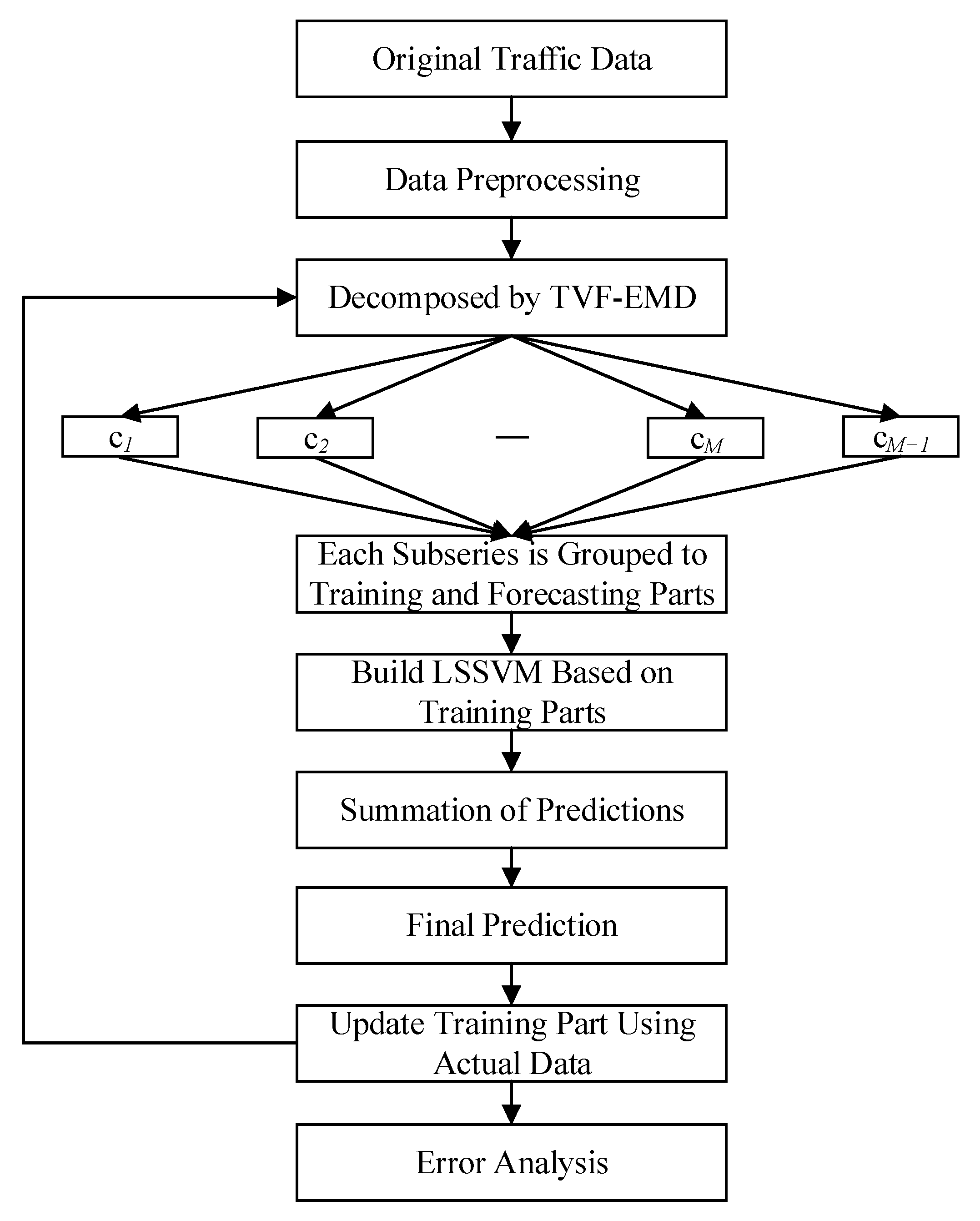
2.3. The Proposed Method

Based on the above discussions, a novel hybrid model which combines the TVF-EMD model and LSSVM model can be developed to improve the forecasting accuracy. First, the TVF-EMD method is presented to deal with the non-stationary and nonlinear traffic volume series. After that, multiple subsequences called narrow-band signals are obtained. Then, the LSSVM model is established for each subsequence. Finally, the prediction results of the subsequences are accumulated to generate the lasted forecasting results. The specific process of TVF-EMD-LSSVM model is shown in Figure 1, and the steps are shown as follows:

Step 1: Preprocess the original traffic volume data with the errors data and missing data to get the experimental data;

Step 2: Decompose the data into several subsequences $\left(\right\{c_j\left(1\right),\dots ,c_j\left(k\right)\},j=1\dots M+1)$ by TVF-EMD algorithm;

Step 3: Divide each subseries into two parts, including training parts $\left\{x^{\prime }\right(1),\dots ,x^{\prime }(k\left)\right\}$ and test parts $\left\{x^{\prime }\right(k+1),\dots ,x^{\prime }(k+N\left)\right\}$;

Step 4: Establish the LSSVM model to predict the $k+1$th data ${\widehat{c}}_j(k+1)$ of subsequences, and sum up to get the forecasting value $\widehat{x}(k+1)$;

Step 5: After updating the training set data to $\left\{x^{\prime }\right(2),\dots ,x^{\prime }(k+1\left)\right\}$, repeat step 2 to step 4 to obtain the prediction results. Continue to predict one step ahead until the prediction task is completed.

3. Case Study

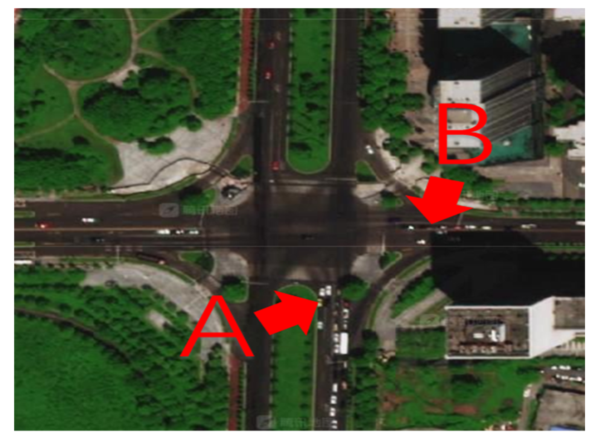
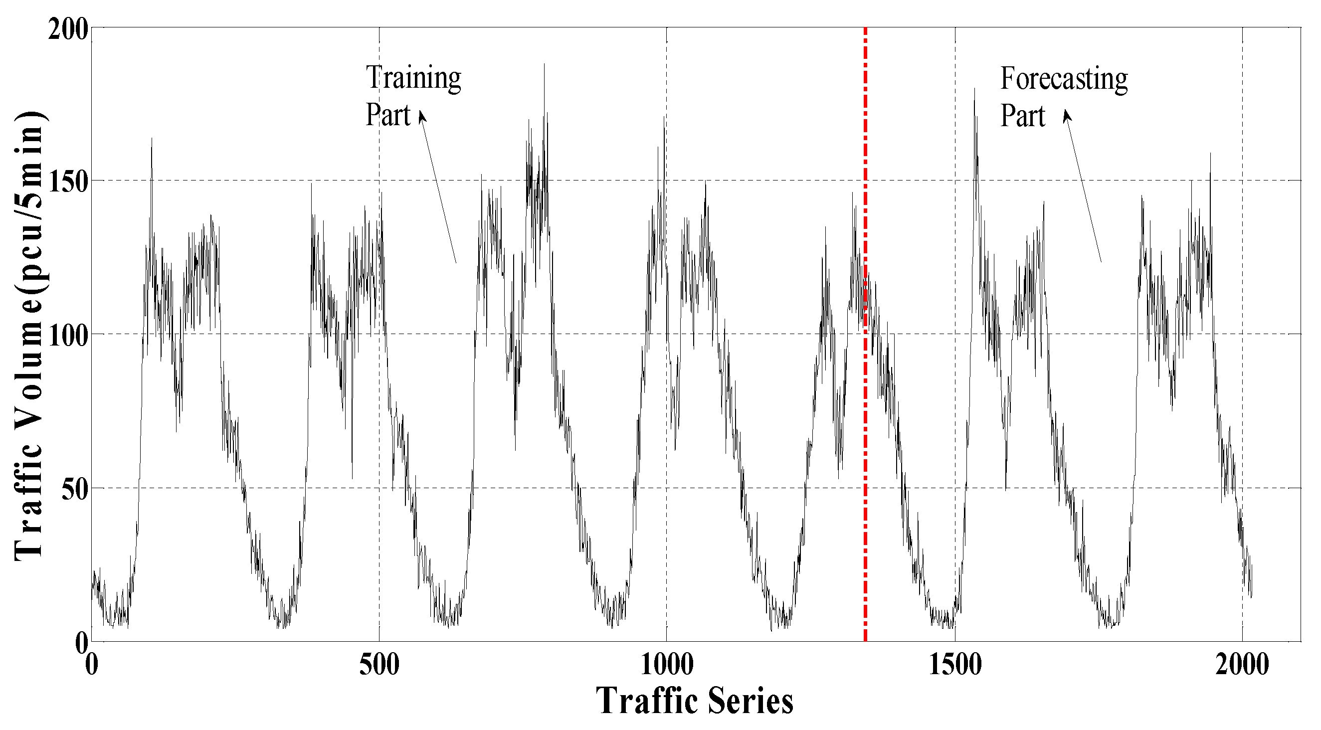
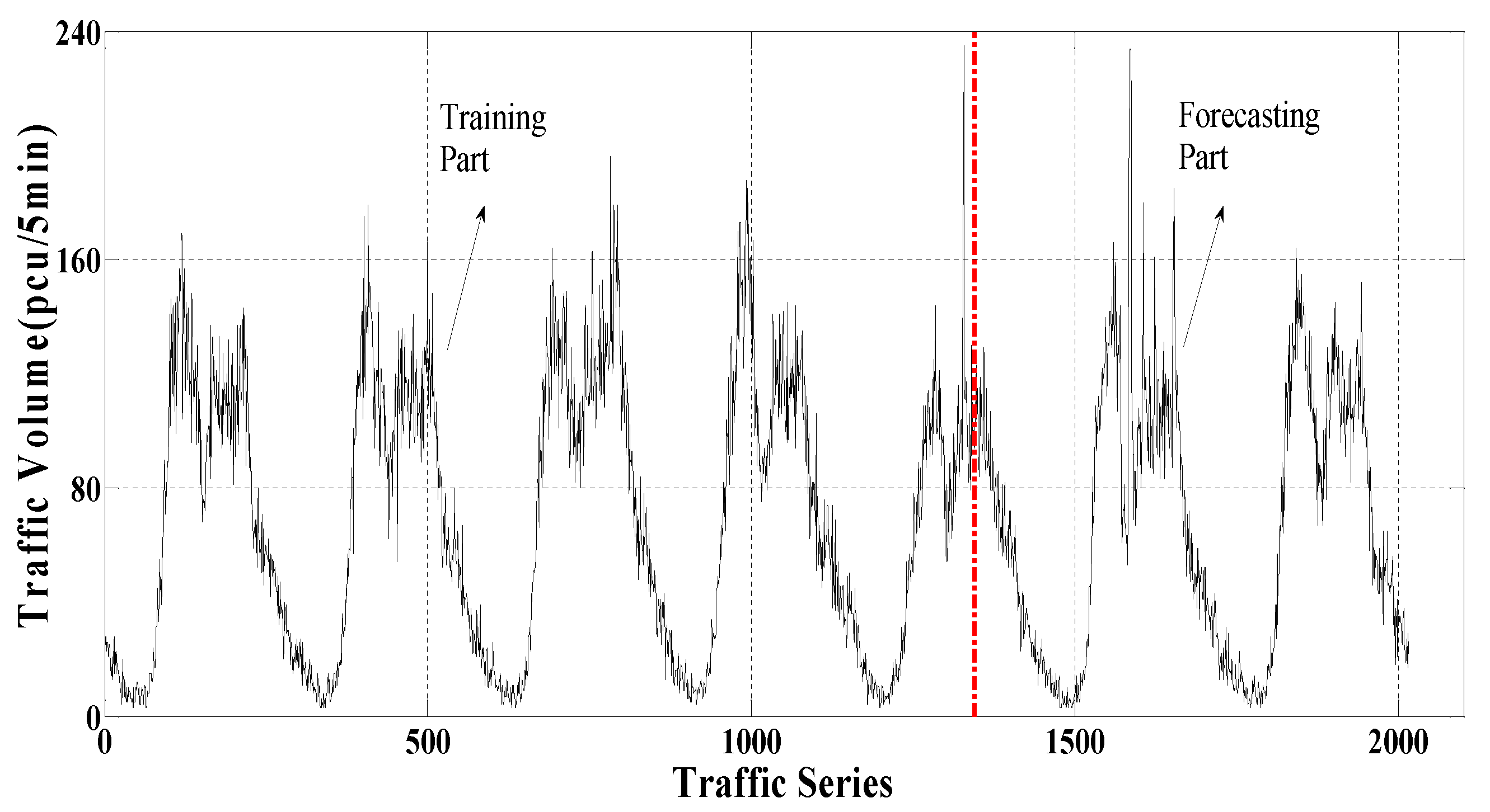
3.1. Data Description

The data collection A (including 2016 samples) was measured from the intersection entrance A of an arterial road in the main urban area of Chongqing and the location is shown in Figure 2. The statistical interval was 5 min, as shown in Figure 3. Two-thirds of the data were used to train the model, and the rest were used to test the performance of the built model.

Table 1. Data characteristics (A).

Data Resource	Mean	Variance	Maximum	Minimum	Skewness	Kurtosis	Non-Stationarity
A	70.184	20,710	188	3	0.0183	1.6495	Strong

summarizes the characteristics of data collection A. It could be observed that this dataset had strong volatility.

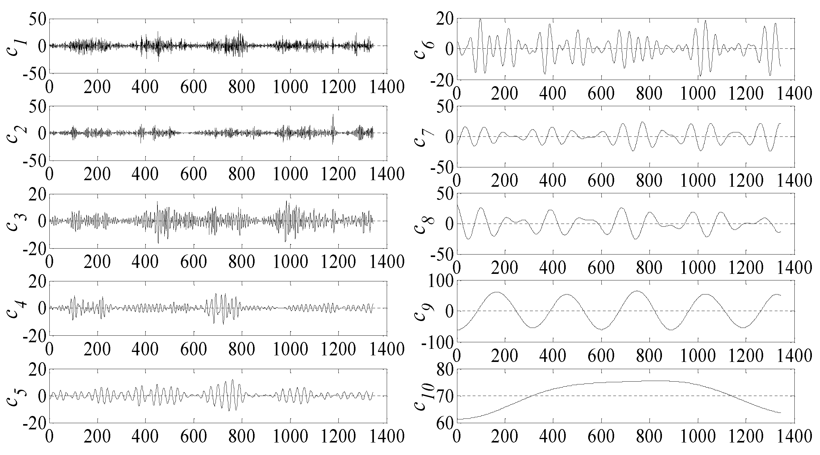
3.2. Data Processing

There are many factors affecting prediction accuracy, such as data quality, data characteristics, and model selection, etc. However, the quality of traffic volume data is one of the main factors [26]. Therefore, the processing of the abnormal data including missing data and erroneous data appears to be crucial in traffic volume prediction [30]. To repair abnormal data, the adjacent completion method is adopted and its function is shown in Equation (14):

$$x\left(t\right)=\left[x\right(t-w)+x(t-w-1)+\cdots +x(t-1\left)\right]/w$$

(14)

where $w$ denotes the number of data to be repaired.

3.3. Evaluation Criteria

In order to analyze and evaluate the forecasting performance of the proposed model, five commonly used evaluation indexes including mean absolute error (MAE), mean relative percentage error (MRPE), root mean square error (RMSE), root mean square relative error (RMSRE) and equal coefficient (EC) were used in the study [26,29]. Their specific definitions are given by:

$$MAE=\frac{1}{n}{\displaystyle \sum _{i=1}^n\left|y_i-{\widehat{y}}_i\right|}$$

(15)

$$MRPE=\frac{1}{n}{\displaystyle \sum _{i=1}^n\left|\frac{y_i-{\widehat{y}}_i}{y_i}\right|}$$

(16)

$$RMSE=\sqrt{\frac{1}{n}{\displaystyle \sum _{i=1}^n{\left(y_i-{\widehat{y}}_i\right)}^2}}$$

(17)

$$RMSRE=\sqrt{\frac{1}{n}{\displaystyle \sum _{i=1}^n{\left(\frac{y_i-{\widehat{y}}_i}{y_i}\right)}^2}}$$

(18)

$$EC=1-\frac{\sqrt{{\displaystyle \sum _{i=1}^n{\left(y_i-{\widehat{y}}_i\right)}^2}}}{\sqrt{{\displaystyle \sum _{i=1}^n{\left(y_i\right)}^2}}+\sqrt{{\displaystyle \sum _{i=1}^n{\left({\widehat{y}}_i\right)}^2}}}$$

(19)

The smaller values of MAE, MRPE, RMSE, and RMSRE indicate the higher accuracy. The closer to one the EC value is, the higher accuracy the prediction is.

3.4. Prediction Results and Analysis

3.4.1. TVF-EMD-LSSVM Model Prediction

According to the forecasting process of the proposed model in Section 2.3, TVF-EMD is used to decompose the experimental data A into 10 subsequences, as shown in Figure 4.

By constructing training and test sets for each subsequence, the LSSVM model is built to predict them. The dimension parameter was determined by minimizing the root mean square error of the output value in the training part [20]. Moreover, the optimal penalty coefficient and kernel function parameters of each subsequence were determined by the optimization function. Finally, the traffic volume prediction value was obtained by accumulating the forecasting results of the subsequences.

3.4.2. Comparison and Analysis of Forecasting Results

To illustrate the performance of the proposed method, three additional forecasting models including ARIMA model, LSSVM model, and EMD-LSSVM model were used to perform the performance comparison. The processes of the LSSVM model, ARIMA model, and EMD-LSSVM model were similar to the forecasting progress in Section 3.4.1. The evaluation indexes of four different models are shown in

Table 2. The comparison results of different methods (A).

Model	MAE	MRPE	RMSE	RMSRE	EC
LSSVM	8.131	17.871%	10.801	27.674%	0.9336
EMD-LSSVM	4.375	9.96%	5.805	15.261%	0.9642
TVF-EMD-LSSVM	1.721	3.969%	2.974	6.797%	0.9816
ARIMA	8.284	17.977%	11.01	27.25%	0.9322

and the corresponding prediction results are shown in Figure 5. From these comparisons, some main observations are provided below:

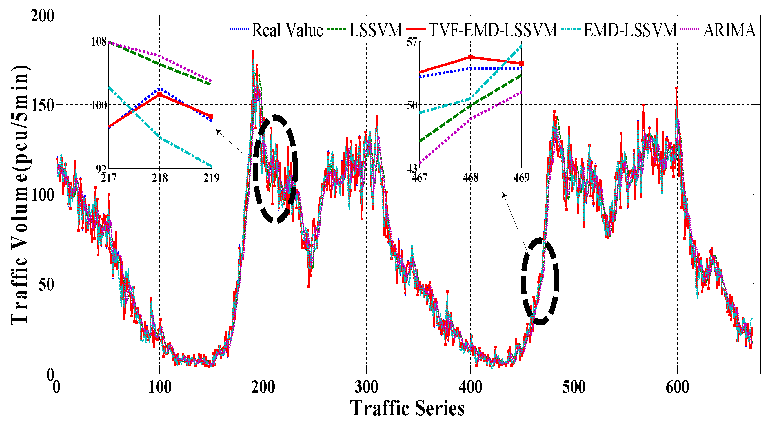
• Compared with the other three involved models, the proposed model had better forecasting performance, where its error indexes of MAE, MRPE, RMSE, RMSRE, and EC were 1.721, 3.969%, 2.974, 6.797%, and 0.9956, respectively. Specifically, in Figure 4, the red line represents the prediction result of the proposed model, while the blue line represents the true value. Their comparison indicates the proposed method could well capture the time-varying characteristics of the actual situation. From Table 2, the forecasting accuracy of the proposed model was higher than the EMD-LSSVM model with the reductions in terms of the five indexes MAE, MRPE, RMSE, RMSRE, and EC by 2.654, 5.991%, 2.831, 8.464%, and 0.0174, respectively. The reason could be that the TVF-EMD algorithm uses time-varying filtering technology, which could describe the time-varying characteristics of the data. Simultaneously, it can improve the imperfection of the model mixing in the EMD algorithm.
• Compared with the single models, the decomposition-based forecasting methods had the higher forecasting accuracy. For example, five error indexes in terms of MAE, MRPE, RMSE, RMSRE, and EC of the LSSVM model were 8.131, 17.871%, 10.801, 27.674%, and 0.9336, respectively, which presents the evident accuracy reduction in comparison with those of the proposed method. Compared with EMD-LSSVM model, these indexes were reduced by 3.756, 7.911%, 4.996, 12.413%, and 0.0306, respectively. The reason for these phenomena could be attributed to high non-stationarity and nonlinear characteristics embedded in the original data, which could be effectively addressed by the decomposition methods.
• The MAE, MRPE, RMSE, RMSRE, and EC of the ARIMA model were 8.284, 17.977%, 11.01, 27.25% and 0.9322. Compared with LSSVM, these indexes were reduced by 0.153, 0.106%, 0.209 0.424, and 0.0014, respectively. The reason could be attributed to that the nonlinear features hidden in the original data were more significant than those of linear one, which leads to the conclusion that the linear ARIMA model cannot capture the characteristics well. Therefore, it owns the lowest forecasting accuracy.

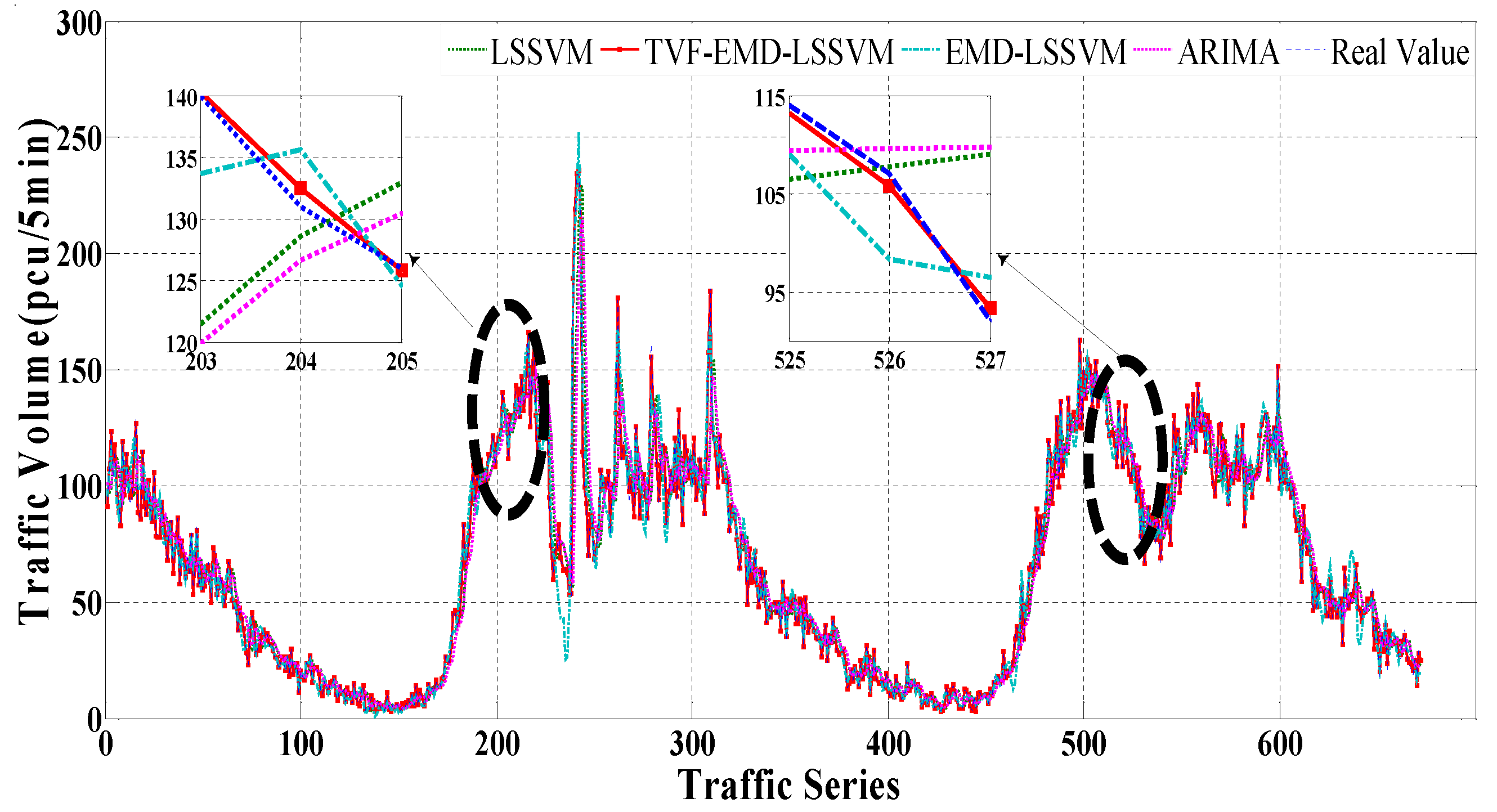
3.5. Additional Case

To further test the stability of the proposed model, another group of data (data collection B) was used. These data were measured from the intersection entrance B of an arterial road in Chongqing (including 2016 samples), as shown in Figure 2 and Figure 6.

Table 3. Data characteristics (B).

Data Resource	Mean	Variance	Maximum	Minimum	Skewness	Kurtosis	Non-Stationarity
B	68.8284	2200.5	235	2	0.2587	2.0441	Strong

provided the relevant information of them. For simplicity, only the error indexes are given in

Table 4. The comparison results of different methods (B).

Model	MAE	MRPE	RMSE	RMSRE	EC
LSSVM	9.281	20.415%	14.787	33.153%	0.8201
EMD-LSSVM	5.93	13.228%	8.405	20.675%	0.8983
TVF-EMD-LSSVM	0.898	2.653%	1.20	5.089%	0.9855
ARIMA	9.584	20.364%	15.762	32.269%	0.808

. The intuitively results are shown in Figure 7. From Table 4 and Figure 7, the main results we

• TVF-EMD was better than EMD in dealing with data nonlinearity and non-stationary. The forecasting result proves that the forecasting accuracy of TVF-EMD based method was higher than EMD based method.
• The hybrid models could take advantage of the superiority each component model. The results display that the forecasting accuracy of the hybrid models was higher than that of the single models.
• The ARIMA model usually presented the high performance for the data with significant linear features. However, for short-term traffic volume data with high nonlinear characteristics, the LSSVM model may have better forecasting performance.

4. Conclusions

In practice, the data of short-term traffic volume commonly owns strong nonlinearity and non-stationarity so that it is hard to provide a satisfactory forecasting result through the traditional methods. In order to improve the forecasting performance, a novel hybrid model based on the combination of TVF-EMD algorithm and LSSVM is developed in this study. Two case studies based on measured data from an intersection are provided to evaluate the performance of the proposed method. Several main conclusions are summarized as follows:

TVF-EMD has a more positive impact than EMD on improving forecasting accuracy. As a newly-improved decomposition method, TVF-EMD can vividly describe the time-varying characteristics (e.g., non-stationarity and nonlinearity) hidden in the data by time-varying filtering technology, where the problems of end effect and model mixing may be well addressed.

The forecasting accuracy of the hybrid models is higher than those of the single models. Generally, the hybrid model could combine the advantages of different component models. In this paper, the advantages of TVF-EMD in processing data non-stationarity and nonlinearity and the merit of LSSVM’s strong ability in addressing the nonlinear problem are combined.

The innovation of this paper is to introduce a new data processing method TVF-EMD algorithm, which improves the model mixing problem of the original EMD algorithm. To further improve the forecasting performance, some future tasks should be carried out. For example, the combination of the proposed method with probabilistic prediction models should be focused; the multi-step ahead prediction will be developed in the future; the application of the proposed method in other fields, such as wind speed prediction and solar radiation prediction, should also be performed.

References

1. Zhang, H.; Wang, X.; Cao, J.; Tang, M.; Guo, Y. A hybrid short-term traffic flow forecasting model based on time series multifractal characteristics. Appl. Intell. 2018, 48, 2429–2440. [Google Scholar] [CrossRef]
2. Liu, Y.; Liu, Z.; Vu, H.L.; Lyu, C. A spatio-temporal ensemble method for large-scale traffic state prediction. Comput. Civ. Infrastruct. Eng. 2020, 35, 26–44. [Google Scholar] [CrossRef]
3. Min, W.; Wynter, L. Real-time road traffic prediction with spatio-temporal correlations. Transp. Res. Part C Emerg. Technol. 2011, 19, 606–616. [Google Scholar] [CrossRef]
4. Kumar, S.V.; Vanajakshi, L. Short-term traffic flow prediction using seasonal ARIMA model with limited input data. Eur. Transp. Res. Rev. 2015, 7, 1–9. [Google Scholar] [CrossRef] [Green Version]
5. Zhao, Z.; Chen, W.; Yue, H.; Liu, Z. A novel short-term traffic forecast model based on travel distance estimation and ARIMA. In Proceedings of the 2016 Chinese Control and Decision Conference (CCDC), Yinchuan, China, 28–30 May 2016. [Google Scholar]
6. Wang, Y.; Li, L.; Xu, X. A piecewise hybrid of ARIMA and SVMs for short-term traffic flow prediction. Lect. Notes Comput. Sci. 2017, 493–502. [Google Scholar] [CrossRef]
7. Wang, Y.; Papageorgiou, M. Real-time freeway traffic state estimation based on extended Kalman filter: A general approach. Transp. Res. Part B Methodol. 2005, 39, 141–167. [Google Scholar] [CrossRef]
8. Okutani, I.; Stephanedes, Y.J. Dynamic prediction of traffic volume through Kalman filtering theory. Transp. Res. Part B 1984, 18, 1–11. [Google Scholar] [CrossRef]
9. Williams, B.M.; Durvasula, P.K.; Brown, D.E. Urban Freeway Traffic Flow Prediction Application of Seasonal Autoregressive Integrated. Transp. Res. Rec. 1998, 1644, 132–141. [Google Scholar] [CrossRef]
10. Kandil, N.; Wamkeue, R.; Saad, M.; Georges, S. An efficient approach for short term load forecasting using artificial neural networks. Int. J. Electr. Power Energy Syst. 2006, 28, 525–530. [Google Scholar] [CrossRef]
11. Ishak, S.; Kotha, P.; Alecsandru, C. Optimization of Dynamic Neural Network Performance for Short-Term Traffic Prediction. Transp. Res. Rec. 2003, 45–56. [Google Scholar] [CrossRef]
12. Vlahogianni, E.I.; Karlaftis, M.G.; Golias, J.C. Optimized and meta-optimized neural networks for short-term traffic flow prediction: A genetic approach. Transp. Res. Part C Emerg. Technol. 2005, 13, 211–234. [Google Scholar] [CrossRef]
13. Zhu, J.Z.; Cao, J.X.; Zhu, Y. Traffic volume forecasting based on radial basis function neural network with the consideration of traffic flows at the adjacent intersections. Transp. Res. Part C Emerg. Technol. 2014, 47, 139–154. [Google Scholar] [CrossRef]
14. Kumar, K.; Parida, M.; Katiyar, V.K. Short term traffic flow prediction in heterogeneous condition using artificial neural network. Transport 2015, 30, 397–405. [Google Scholar] [CrossRef]
15. Wu, C.H.; Wei, C.C.; Su, D.C.; Chang, M.H.; Ho, J.M. Travel time prediction with support vector regression. IEEE Conf. Intell. Transp. Syst. Proc. ITSC 2003, 2, 1438–1442. [Google Scholar] [CrossRef] [Green Version]
16. Wang, J.; Shi, Q. Short-term traffic speed forecasting hybrid model based on Chaos-Wavelet Analysis-Support Vector Machine theory. Transp. Res. Part C Emerg. Technol. 2013, 27, 219–232. [Google Scholar] [CrossRef]
17. Cong, Y.; Wang, J.; Li, X. Traffic Flow Forecasting by a Least Squares Support Vector Machine with a Fruit Fly Optimization Algorithm. Procedia Eng. 2016, 137, 59–68. [Google Scholar] [CrossRef] [Green Version]
18. Luo, C.; Huang, C.; Cao, J.; Lu, J.; Huang, W.; Guo, J.; Wei, Y. Short-Term Traffic Flow Prediction Based on Least Square Support Vector Machine with Hybrid Optimization Algorithm. Neural Process. Lett. 2019, 50, 2305–2322. [Google Scholar] [CrossRef]
19. Shang, Q.; Lin, C.; Yang, Z.; Bing, Q.; Zhou, X. Short-term traffic flow prediction model using particle swarm optimization-based combined kernel function-least squares support vector machine combined with chaos theory. Adv. Mech. Eng. 2016, 8, 1–12. [Google Scholar] [CrossRef] [Green Version]
20. Jiang, Y.; Huang, G. Short-term wind speed prediction: Hybrid of ensemble empirical mode decomposition, feature selection and error correction. Energy Convers. Manag. 2017, 144, 340–350. [Google Scholar] [CrossRef]
21. Shang, Q.; Lin, C.; Yang, Z.; Bing, Q.; Zhou, X. A hybrid short-term traffic flow prediction model based on singular spectrum analysis and kernel extreme learning machine. PLoS ONE 2016, 11, 1–25. [Google Scholar] [CrossRef]
22. Labate, D.; Foresta, F.L.; Occhiuto, G.; Morabito, F.C.; Lay-Ekuakille, A.; Vergallo, P. Empirical mode decomposition vs. wavelet decomposition for the extraction of respiratory signal from single-channel ECG: A comparison. IEEE Sens. J. 2013, 13, 2666–2674. [Google Scholar] [CrossRef]
23. Huang, N.E.; Shen, Z.; Long, S.R.; Wu, M.C.; Snin, H.H.; Zheng, Q.; Yen, N.C.; Tung, C.C.; Liu, H.H. The empirical mode decomposition and the Hubert spectrum for nonlinear and non-stationary time series analysis. Proc. R. Soc. Math. Phys. Eng. Sci. 1998, 454, 903–995. [Google Scholar] [CrossRef]
24. Duo, M.; Qi, Y.; Lina, G.; Xu, E. A short-term traffic flow prediction model based on EMD and GPSO-SVM. In Proceedings of the 2017 IEEE 2nd Advanced Information Technology, Electronic and Automation Control Conference, Chongqing, China, 25–26 March 2017. [Google Scholar]
25. Tang, J.; Chen, X.; Hu, Z.; Zong, F.; Han, C.; Li, L. Traffic flow prediction based on combination of support vector machine and data denoising schemes. Phys. Stat. Mech. Appl. 2019, 534, 120642. [Google Scholar] [CrossRef]
26. Tian, X.; Yu, D.; Xing, X.; Wang, S.; Wang, Z. Hybrid short-term traffic flow prediction model of intersections based on improved complete ensemble empirical mode decomposition with adaptive noise. Adv. Mech. Eng. 2019, 11, 1–15. [Google Scholar] [CrossRef]
27. Li, H.; Li, Z.; Mo, W. A time varying filter approach for empirical mode decomposition. Signal Process. 2017, 138, 146–158. [Google Scholar] [CrossRef]
28. Zhang, X.; Liu, Z.; Miao, Q.; Wang, L. An optimized time varying filtering based empirical mode decomposition method with grey wolf optimizer for machinery fault diagnosis. J. Sound Vib. 2018, 418, 55–78. [Google Scholar] [CrossRef]
29. Jiang, Y.; Zhao, N.; Peng, L.; Liu, S. A new hybrid framework for probabilistic wind speed prediction using deep feature selection and multi-error modification. Energy Convers. Manag. 2019, 199, 111981. [Google Scholar] [CrossRef]
30. Li, L.; Su, X.; Wang, Y.; Lin, Y.; Li, Z.; Li, Y. Robust causal dependence mining in big data network and its application to traffic flow predictions. Transp. Res. Part C Emerg. Technol. 2015, 58, 292–307. [Google Scholar] [CrossRef]
Figure 1. The procedure of time varying filtering based empirical mode decomposition and least square support vector machine (TVF-EMD-LSSVM).
Applsci 10 02038 g001
Figure 2. Location of the intersection in Chongqing.
Applsci 10 02038 g002
Figure 3. Traffic volume time series (A).
Applsci 10 02038 g003
Figure 4. The pictures of TVF-EMD decomposition results (A).
Applsci 10 02038 g004
Figure 5. The predictions of different methods (A).
Applsci 10 02038 g005
Figure 6. Traffic volume time series (B).
Applsci 10 02038 g006
Figure 7. The predictions of different methods (B).
Applsci 10 02038 g007