Article

Seasonal and Long-Term Trend of on-Road Gasoline and Diesel Vehicle Emission Factors Measured in Traffic Tunnels

1
Center for Atmospheric Particle Studies, Carnegie Mellon University, Pittsburgh, PA 15213, USA
2
Department of Mechanical Engineering, Carnegie Mellon University, Pittsburgh, PA 15213, USA
3
South Coast Air Quality Management District, Diamond Bar, CA 91765, USA
4
International Council on Clean Transportation, Washington, DC 20005, USA
5
Department of Civil, Environmental and Geodetic Engineering, The Ohio State University, Columbus, OH 43210, USA
*
Author to whom correspondence should be addressed.
Submission received: 29 February 2020 / Revised: 25 March 2020 / Accepted: 27 March 2020 / Published: 3 April 2020
(This article belongs to the Special Issue Combustion Aerosol)

Abstract

:
Emissions of gaseous and particulate pollutants from on-road gasoline and diesel vehicles were measured in a traffic tunnel under real-world driving conditions. Emission factors were attributed to gasoline and diesel vehicles using linear regression against the fraction of fuel consumed by diesel vehicles (% fuelD). We measured 67% higher NOx emissions from gasoline vehicles in winter than in spring (2 versus 1.2 g NO2 kg fuel−1). Emissions of CO, NOx, and particulate matter from diesel vehicles all showed impacts of recent policy changes to reduce emissions from this source. Comparison of our measurements to those of a previous study ~10 years prior in a nearby traffic tunnel on the same highway showed that emission factors for both gasoline and diesel vehicles have fallen by 50–70%. To further confirm this long-term trend, we summarized emission factors measured in previous tunnel studies in the U.S. since the 1990s. More restrictive emission standards are effective at reducing emissions from both diesel and gasoline vehicles, and decreases in observed emissions can be mapped to specific vehicle control policies. The trend of diesel-to-gasoline emission factor ratios revealed changes in the relative importance of vehicle types, though fuel-specific emission factors of NOx and elemental carbon (EC) are still substantially larger (~5–10 times) for diesel vehicles than gasoline vehicles.

1. Introduction

On-road gasoline and diesel vehicles are a major source of air pollutants in the urban atmosphere [1,2]. Approximately 37% of CO emissions, 14% of Volatile Organic Compound (VOC) emissions, 39% of NOx emissions, and 3% of primary fine particle (PM2.5) emissions were contributed by on-road gasoline and diesel vehicles in the United States in 2014 [1]. These pollutants are important participants in atmospheric chemical reactions and have adverse effects on human health. NOx and VOC are important precursors to tropospheric ozone (O3) [3], which can lead to lung function damage and cause respiratory diseases.
PM2.5 impacts climate by scattering or absorbing solar radiation [4,5], and exposure to PM2.5 is detrimental to health [6,7]. Roughly 50% of fine particle mass is constituted by organic species, i.e., organic aerosol (OA) or organic carbon (OC) [8,9]. In addition to OC, PM emissions from vehicles also mainly consist of carbon soot, which is also known as elemental carbon (EC) or black carbon (BC) [10].
Gasoline and diesel vehicles have distinctive emission characteristics because of differences in engine technology. Gasoline vehicles are powered by spark-ignition (SI) engines, while diesel vehicles are powered by compression-ignition (CI) engines. The local fuel-rich conditions and the high combustion temperature of the CI engine favor the formation of PM and NOx [11]. The overall fuel-to-air ratio in SI engines is higher than in CI engines, and there is not enough time in SI engine to convert all CO to CO2 [11]. Gasoline vehicles emit more CO than diesel vehicles, while uncontrolled diesel vehicles emit much higher NOx and PM than gasoline vehicles [12,13,14,15]
Numerous studies have been conducted to measure vehicle emissions, including dynamometer studies [13,16,17], on-road and near-road measurements [18,19,20,21,22], vehicle chase studies [23,24,25], and tunnel studies [12,14,26,27,28,29,30,31,32,33]. On-road and near-road studies include measurements with portable emissions measurement systems (PEMS) [34] and remote sensing [35]. Dynamometer studies, in which the vehicle exhaust is sampled under a prescribed driving cycle, offer controlled sampling conditions, though questions remain whether dynamometer tests are representative of real-world driving conditions. In addition, the vehicle population sampled in a typical dynamometer campaign is tiny compared with the real-world traffic volume. For on-road, near-road, and vehicle chase studies, the vehicle exhaust is sampled under real-world driving conditions. Tunnel and near-road studies typically sample from large vehicle fleets, but these studies have to account for the dilution of emissions with background air.
Tunnel studies offer real-world driving conditions and a large-volume traffic fleet. The primary advantages of tunnel studies are that the emissions are less diluted than in near-road conditions and that a large vehicle fleet can be sampled under realistic driving conditions. A major challenge of tunnel studies is to separate the gasoline and diesel vehicle emissions from a mixed fleet [33]. Also, since many tunnel studies sample from highway tunnels, only emissions from high-speed driving are characterized. Thus, tunnel measurements typically do not capture emissions at low speed or vehicle cold starts, operation modes that can have significantly different emissions rates than high-speed driving [13,17].
Previous studies have suggested that ambient temperature can affect vehicle emissions; this in turn would drive seasonal variations in on-road vehicle emissions. Nam et al. [16] tested 496 vehicles on a chassis dynamometer under summer and winter ambient temperature. They found that PM emissions from gasoline-powered vehicles increased dramatically with decreased temperature, and the temperature effects on PM emissions were most significant during the vehicle cold-start phase. Saha et al. [22] and Wang et al. [36] conducted near-road measurements and measured higher emissions of NOx and particle number in winter than summer, but higher emissions of particulate BC in summer. Grange et al. [37] observed that NO2 emissions from light-duty diesel vehicles increased with decreasing temperature. Grieshop et al. [14] measured vehicle emission factors in a traffic tunnel and found that during the rush-hour period, the PM2.5 mass emission factor and the EC emission factor were lower in winter than in summer, but the OC emission factor was higher in winter.
Although previous lab and field studies found that emission factors of on-road vehicles may have seasonal variations, vehicle emission models do not always use seasonally dependent emission factors. The MOtor Vehicle Emission Simulator (MOVES) developed by US EPA (Environmental Protection Agency) and the EMission FACtors (EMFAC) model developed by the California Air Resources Board (CARB) are two widely used vehicle emission models. MOVES uses seasonally independent emission factors [38]. EMFAC uses different emission rates for different seasons, since fuel composition is different in summer and winter in the state of California [39].
The purpose of this study is to quantify vehicle emissions under real-world driving conditions and current fleet composition. We conducted multi-seasonal measurements in the Fort Pitt Tunnel in Pittsburgh, PA, which allowed us to investigate potential seasonal variations of vehicle emissions. The fleet average emission factors were combined with traffic data to apportion the fuel-based emission factors of gasoline and diesel vehicles. In order to study the long-term trend of vehicle emissions, we compared our emissions measurements to those of previous U.S. tunnel studies over the past three decades, including an earlier study in Pittsburgh [14]. We also compared the vehicle emission factors measured in traffic tunnels to emission factors simulated by MOVES.

2. Methods

2.1. The Fort Pitt Tunnel

The measurement campaign was conducted in the two-lane outbound (westbound) bore of the Fort Pitt Tunnel on Interstate 376 in Pittsburgh, PA. The tunnel is 1.1 km long with a 2.5% uphill grade. It connects the downtown area of Pittsburgh to the Pittsburgh International Airport and other suburban areas. Continuous spring measurements were conducted in April and May 2013, together with the work presented in Li et al. [40] and Tkacik et al. [41], and continuous winter measurements were conducted in January and February 2014. A one-week measurement was conducted in the period 29 April–4 May, 2014, in order to study the difference of emission factors measured over different traffic lanes, as described in detail later. A detailed description of the Fort Pitt Tunnel, the tunnel measurement station, and the traffic conditions in the tunnel can be found in Li et al. [40]
We quantified the presence of diesel vehicles by calculating the diesel fuel fraction (% fuelD) with the following equation:
% f u e l D = f D U D f D U D + ( 1 f D ) U G
The % fuelD represents the percentage of fuel consumed by heavy duty diesel vehicles (HDDV). Here fD is the number fraction of diesel vehicles determined based on traffic counts obtained from the Pennsylvania Department of Transportation at the tunnel exit. UG and UD are the fuel economies of gasoline vehicles (25 mile/gallon) and diesel vehicles (6 mile/gallon), calculated based on the total vehicle-mileage data and total fuel consumption data of light duty vehicles and trucks in 2011 from the US Department of Transportation [42].

2.2. Air Quality Measurement Station

As described in Li et al. [40], for both the winter and the spring campaigns, we had one gas-phase sampling line (0.25 in. diameter Teflon tubing) for all gas monitors and one particle-phase sampling line (0.325 in. diameter copper tubing) for all particle instruments.
During the spring campaign, we continuously measured CO2 (LiCor Li-820), CO (Teledyne-API T300), NOx (= NO + NO2; Teledyne-API 200EU), and particle-phase OC and EC concentrations in the tunnel. All gases were measured at 1 second resolution. Particle-phase OC and EC were measured with a semi-continuous OC/EC analyzer (Sunset Laboratories) operating at hourly resolution. A denuder was placed upstream of the OC/EC analyzer to remove vapor-phase organics and reduce sampling artifacts. The sampling inlet was over the left lane, and the sampling lines were about 22 m long due to constraints on where the instruments could be deployed. The Reynolds number of the particle sampling line was less than 2000, indicating the airflow inside was laminar flow. The long length of the particle-phase sampling line may potentially lead to a high particle loss for smaller particles. Smaller particles are negligible in mass, so any losses should have a minor impact on the measured particle mass concentration.
During the winter campaign, in order to better capture emissions from heavy-duty diesel vehicles (HDDV), the sampling inlet was placed on top of the right lane, where most trucks drive. All instruments were also moved next to the sampling inlet to minimize the length of the sampling line (<2 m), reduce losses, and capture exhaust plumes from individual trucks.
During the winter campaign, the denuder placed upstream of the OC/EC analyzer became saturated. Therefore, in order to constrain potential sampling artifacts, we collected quartz filter sets for offline OC/EC analysis, as described by Li et al. [40] As shown in Figure S1 in the Supporting Information, we used the correlation between concurrent measurements of OC on filters and from the semi-continuous OC/EC analyzer to determine an empirical artifact correction for the winter measurement period.

2.3. Fuel-Based Emission Factors

Emission factors reported in this work are fuel-based emission factors calculated using the following equation, which assumes a carbon balance between the fuel and the combustion exhaust:
E F P = Δ P Δ C O 2 + Δ C O M W P M W C ω C
EFp is the emission factor of pollutant P (in g/kg-fuel). ∆P, ∆CO2, and ∆CO are background corrected concentrations of P, CO2, and CO. MWp and MWc are molecular weights of pollutant P and carbon, wc is the weight fraction of carbon in the fuel. The wc of gasoline and diesel are 0.85 and 0.87, respectively; wc values at each hour of the day in the tunnel were calculated as the weighted average wc based on the % fuelD. This method assumes that the carbon in the fuel was dominantly transformed into CO2 and CO during combustion and that VOCs and particle-phase OC and EC are negligible for the carbon balance. Following previous studies, we report NOx emissions in NO2 equivalents (e.g., g-NO2/kg-fuel).

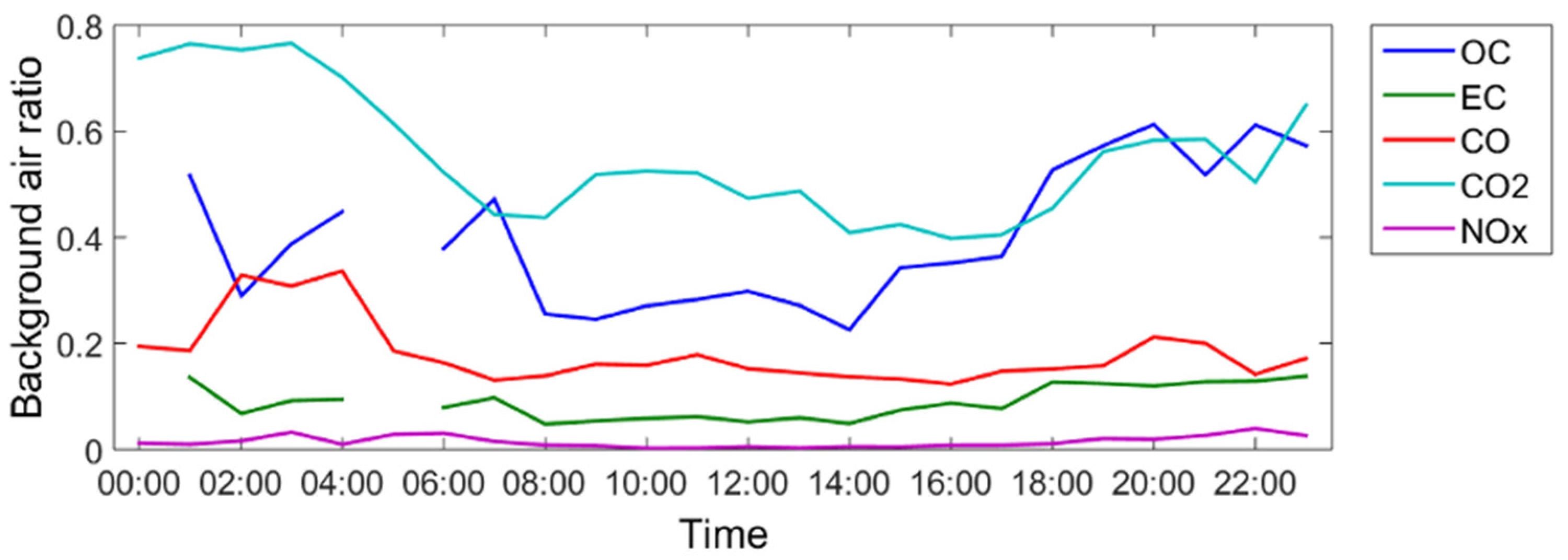
2.4. Background Pollutant Concentrations

The background pollutant concentrations used in this work were the ambient monitoring data from nearby U.S. EPA air monitoring sites. The data were obtained from the EPA Air Quality System (AQS). NOx and CO background concentrations came from monitoring data at the Carnegie Science Center site (40.4456° latitude, −80.0162° longitude), which is ~900 m away from the Fort Pitt Tunnel. For the particle-phase OC and EC concentrations, we used the ambient monitoring data from the Lawrenceville site (40.4654° latitude, −79.9608° longitude). This site is ~5 km away from the tunnel and is representative of urban background concentrations in Pittsburgh.
Background CO2 concentrations were measured on the campus of Carnegie Mellon University with a Li-Cor LI-820 CO2 monitor at 1 Hz from 29 April to 17 May, 2014. Diurnal patterns of weekday and weekend CO2 ambient concentrations were used to background correct the CO2 concentrations measured in the tunnel. We assumed that these data were relevant for background correction of both spring and winter measurements.
The pollutant concentrations measured in the tunnel were in general much larger than the ambient background concentrations. In Figure 1, we present the diurnal average fraction of background air contribution to each of the measured pollutants. The NOx background concentrations were less than 3% of the tunnel measurement, and the EC background concentrations were around 10%. CO had a higher background contribution, around 20% during the day and 30% in the early morning hours (02:00–04:00). OC and CO2 had the highest contributions from the background. The OC background ratios were 40–60%.

3. Results and Discussion

3.1. Pollutant Concentrations and Emission Factors

The background-corrected time series of gaseous and particulate pollutants measured in the tunnel in a typical week (3 February to 9 Feb, 2014) are presented in Figure S2. All measured species showed strong diurnal patterns, and these diurnal trends are good indicators of the traffic conditions. CO2 and CO concentrations showed two peaks during weekdays, one during the morning rush hour (around 08:00), and the other one in the afternoon rush hour (15:00–17:00). During weekends, these species presented only one peak during the afternoon. These trends are consistent with the overall traffic patterns, driven by the number of gasoline vehicles.
The time series of NOx, OC, and EC concentrations showed a different temporal pattern than CO and CO2. On weekdays, NOx, OC, and EC had only one peak around midday. This seemed to be associated with diesel truck activity, since the peak volume of HDDV in the tunnel was also around noon. Weekend concentrations of NOx were generally much lower than on weekdays, consistent with reduced HDDV traffic. One exception occurred on Saturday at ~01:00–02:00, when a spike in NOx and CO was observed. This spike may be indicative of high diesel truck volumes during that specific time.
The hourly averaged diurnal patterns of NOx, OC, EC, and CO emission factors measured on weekdays in the spring campaign are presented in Figure 2. The diurnal trends of emission factors measured in the winter campaign were similar. Unlike the NOx, OC, and EC concentrations, which followed the trend of the HDDV volume and peaked around midday, the NOx, OC, and EC emission factors closely followed the trend of the % fuelD and had the highest value during overnight hours (0:00–4:00), dropping by about 65% in daytime. This is because HDDV emit much higher NOx, OC, and EC than light-duty gasoline vehicles (LDV), and the fraction of HDDV in the tunnel was much higher during overnight hours than in daytime.
The diurnal trends of NOx, OC, and EC emission factors measured in this study are similar to those measured by Grieshop et al. [14] at a nearby Pittsburgh tunnel in 2002. They separated the measured emission factors into three time periods—the early morning (high truck, 0:00–06:00), morning rush hour (low speed, 07:00–09:00), and midday (high speed, 10:00–16:30)—and found that the NOx, OC, and EC emission factors were much higher in the early morning than in other time periods and the emission factors in the rush hour were slightly lower than at midday, since the % fuelD was lower during rush hour.
Unlike NOx, OC, and EC, the diurnal pattern of the CO emission factors measured in the tunnel does not follow the trend of % fuelD. The hourly averaged CO emission factors were relatively constant during the entire day, suggesting that CO emissions trends are driven by LDV. From midnight to 3 am, the CO emission factors were slightly higher and more variable. It may be because during these hours, the background CO ratio was also higher (Figure 1) and the calculated CO emission factors were more subject to the influence of the background air.

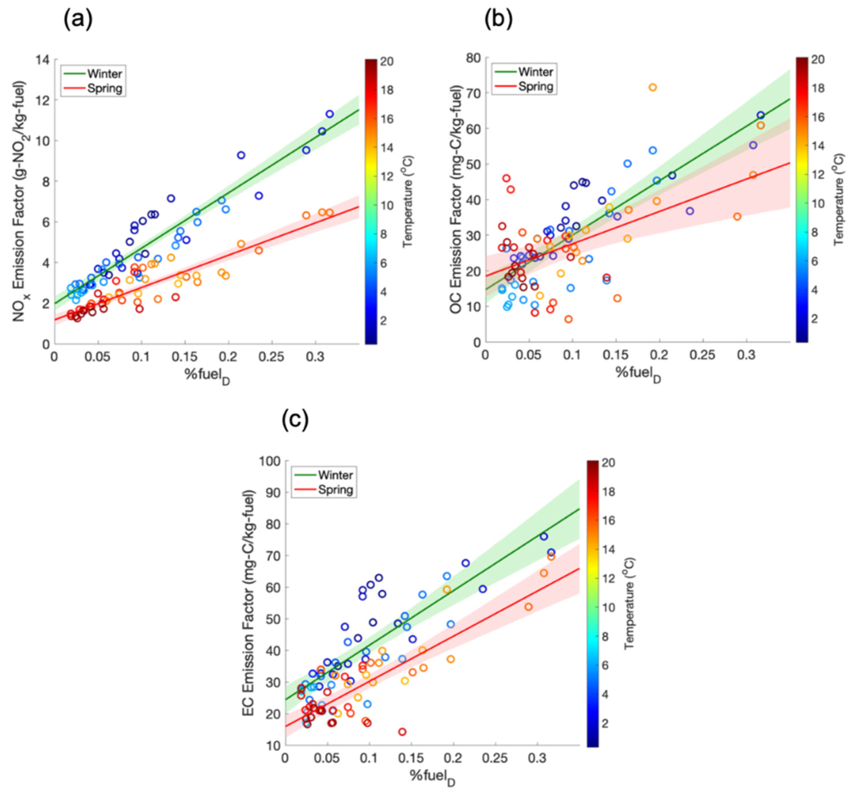
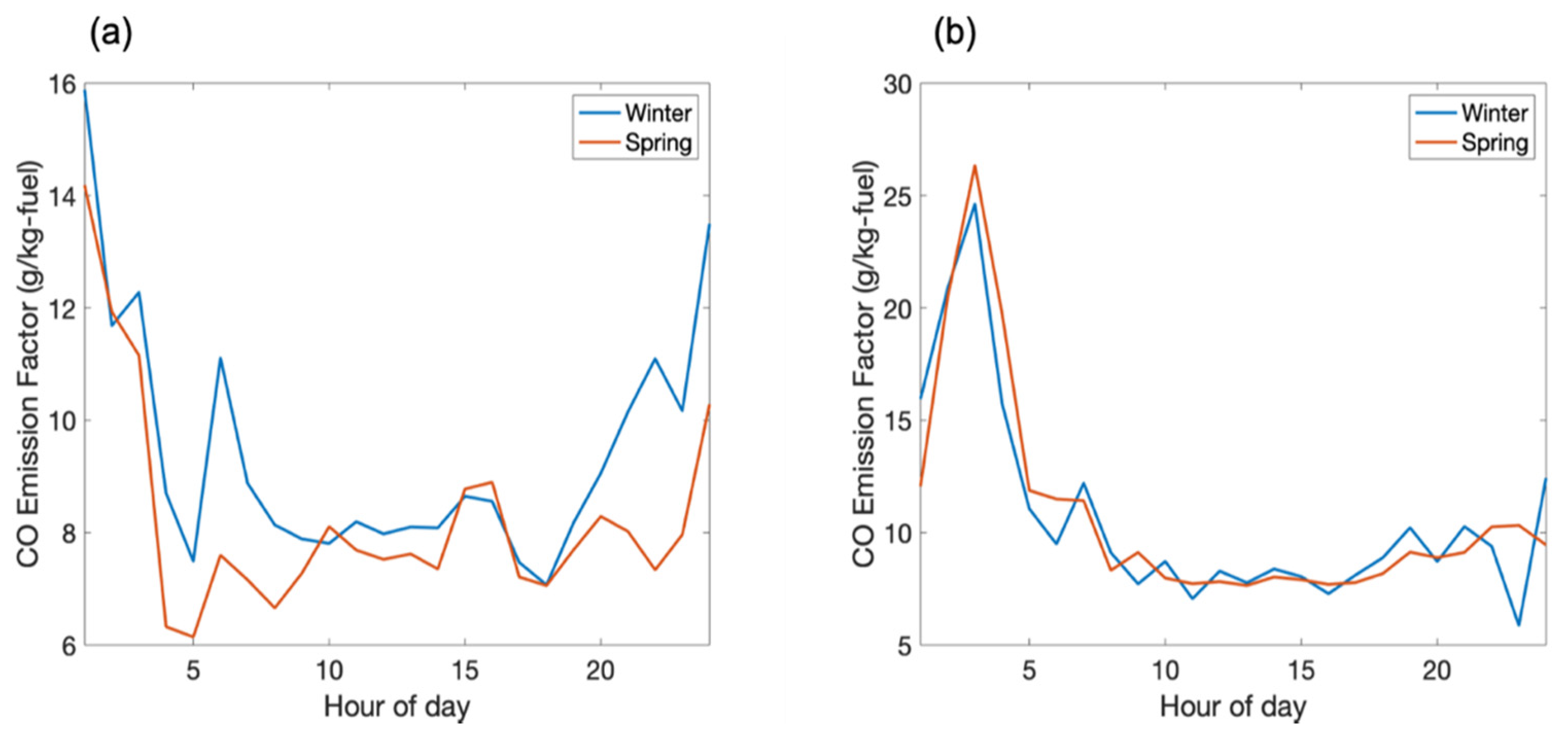
3.2. Seasonal Variation of Emission Factors

As discussed above, the hourly averaged emission factors shown in Figure 2 are mixed emission factors of gasoline and diesel vehicles and were greatly affected by % fuelD. In order to remove the dependence of emissions factors on % fuelD and directly show the potential seasonal trend, in Figure 3, we performed a linear regression of emission factors as a function of % fuelD. The linear regression was performed separately for winter and spring measurements. It was performed for NOx, OC, and EC in the % fuelD range of 0%–40%. The data points used for the linear regression were hourly averaged diurnal emission factors and hourly averaged % fuelD. The uncertainty of the linear regression was calculated as the simultaneous functional bounds of the linear fit at the 95% confidence level.
As shown in Figure 3, we observed a seasonal variation in emissions of NOx and EC. NOx and EC emissions were both elevated in winter for the entire % fuelD range. The NOx emission factor we measured in winter was, on average, 1.7 times larger than in spring at all % fuelD, which is larger than the seasonal changes measured by Wang et al. (50%) [36] and Saha et al. (13%) [22]. Regardless of absolute differences, our results contribute to the growing body of evidence that on-road vehicle NOx emissions are higher in winter.
We measured EC emission factors in winter that were 1.4 times higher than in spring, whereas Wang et al. [36] and Saha et al. [22] measured slightly lower wintertime emissions. Uncertainty ranges of the NOx and EC emission factors we measured in winter and spring did not overlap, except for EC emission factor at % fuelD = 0 (i.e., our estimated EC emissions for gasoline vehicles). OC emissions, on the other hand, were not systematically different between winter and spring.
The spring and winter measurements were conducted over left and right lanes, respectively. Since diesel trucks are expected to primarily travel in the right lane, there is a possibility that the higher emission factors measured during winter are simply a result of the traffic distribution between lanes. Therefore, we further verified that the seasonal variation of emission factors was not an artifact of sampling over different lanes. We collected data during weekdays in a single week in spring 2014 and compared the diurnal pattern of NOx emission factors measured over left and right lanes in Figure S3. Overall, there was good agreement. From 5:00 to 20:00, emission factors over the two lanes were identical within experimental uncertainty. The % fuelD ranged from 3% to 13% over this time. NOx emissions measured over the right lane were 30–40% higher between 20:00 and 3:00, when % fuelD was between 7% and 30%. Some of this difference is likely attributable to the right lane having more diesel trucks, but some of the difference (e.g., higher emission factors from 20:00 to 21:00 when % fuelD < 10%) may be due to lower pollutant concentrations and higher background ratios. Figure S3 suggests that the differences in emission factors shown in Figure 3 for % fuelD <13% are robust but that the difference in emission factors for periods with higher diesel activity (e.g., >20%) may be exaggerated by the lane difference. Since the LDV emission factors can be determined from the regressions when % fuelD is 0, we assume that the seasonal trend presented in Figure 3 is valid for LDV. LDV emission factors measured in winter and spring are summarized in Table 1.
As shown in Figure 2d, the CO emission factor was not correlated with % fuelD. We therefore assessed the potential seasonal variation of the CO emission factor by directly comparing the weekday and weekend diurnal patterns of CO emission factors measured in winter and spring. The results are shown in Figure 4. The CO emission factors were in general similar in winter and spring. During 8:00–19:00 on weekdays and 1:00–21:00 on weekends, when LDV dominate the traffic flow, CO emission factors were similar (in general, less than 10% difference) in winter and spring. During 20:00–7:00 on weekdays, when both the fraction of LDV in the traffic flow and the total traffic volume are lower, CO emission factors were slightly higher (10–51%) in winter than in spring. Wang et al. [36] also reported similar CO emission factors across different seasons.

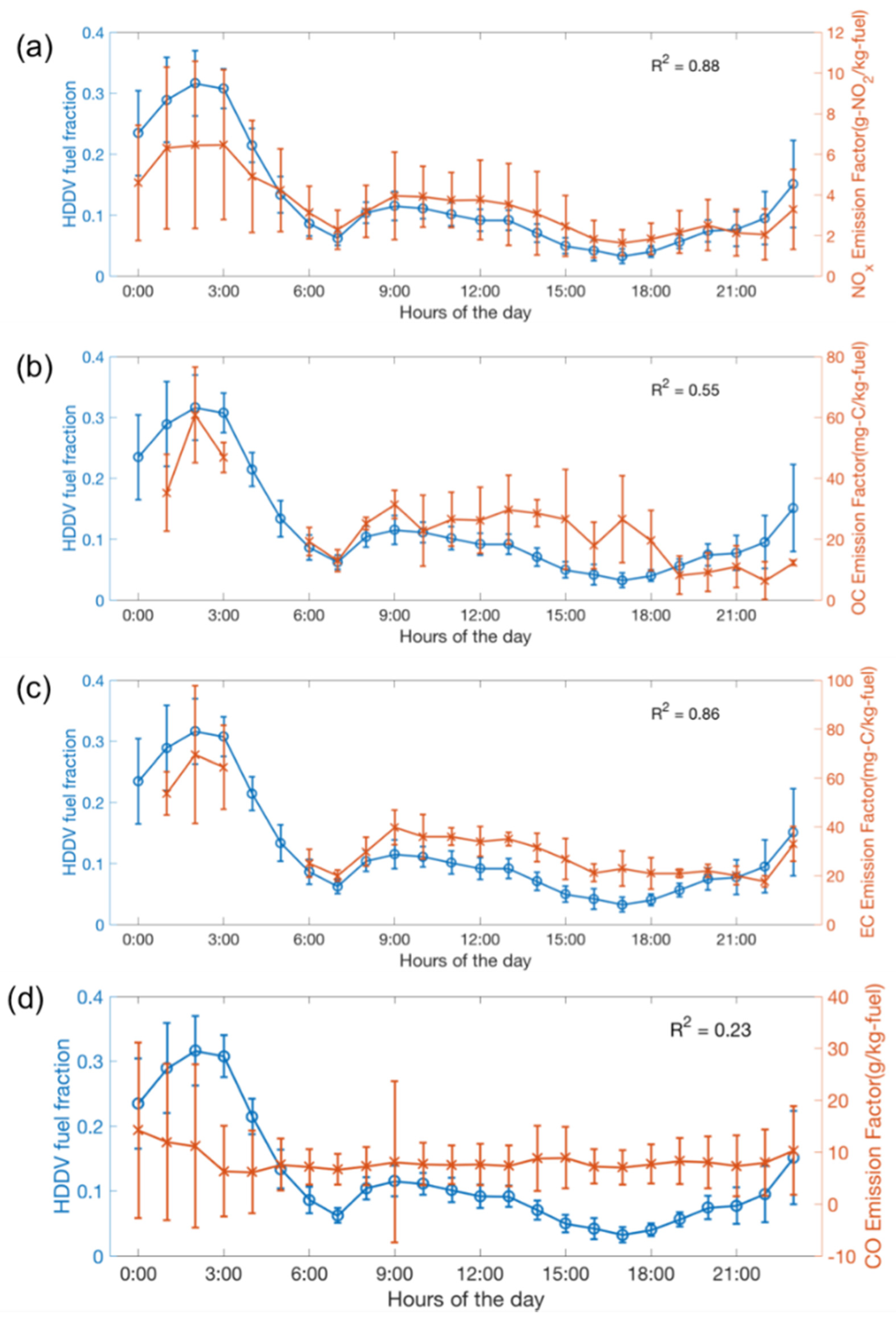
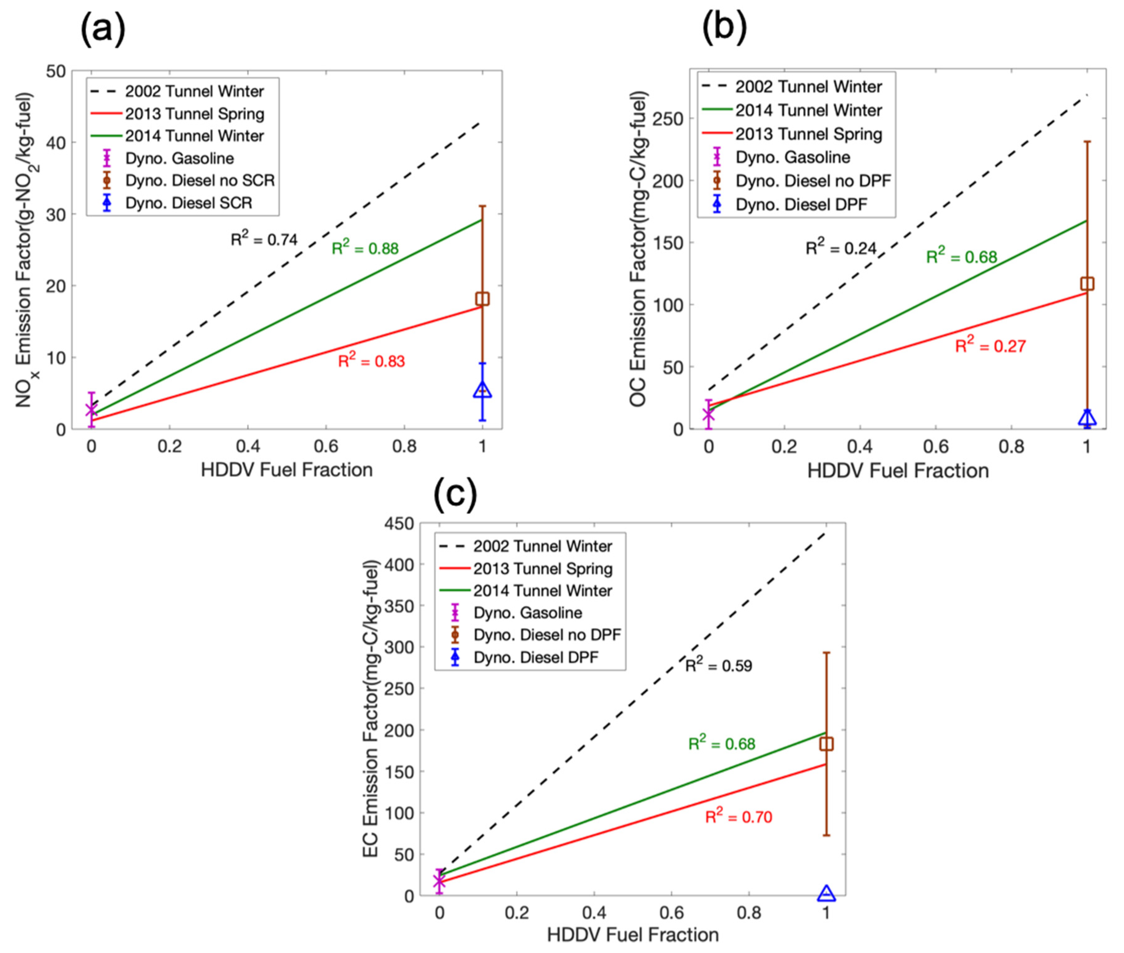
3.3. Emission Factors of LDV and HDDV

The hourly averaged emission factors shown in Figure 2 are mixed emission factors of gasoline and diesel vehicles. They cannot be directly compared with other tunnel studies, since different tunnels may have different traffic volumes and vehicle composition (% fuelD). The strong correlations between the emission factors and the % fuelD, especially for NOx, OC, and EC, offer a chance to apportion LDV and HDDV emissions. Following previous studies [14,43,44], we extended the linear regression shown in Figure 3 to the % fuelD range of 0 to 1 to extrapolate the LDV emission factor (% fuelD = 0) and the HDDV emission factor (% fuelD = 1). The results of linear regressions are presented in Figure 5, and the uncertainty ranges of linear regressions are presented in Figure S4.
An advantage of using the linear regression to determine LDV and HDDV emission rates is that it allows us to compare them directly to measurements by Grieshop et al. [14], which were conducted in a different tunnel (Squirrel Hill tunnel) on the same highway (I-376) in Pittsburgh ~10 years prior to our measurements. Emission factors from Grieshop et al. [14] are shown as black dashed lines in Figure 5. These paired studies show that over the course of ~10 years, emissions of NOx, OC, and EC from LDV and HDDV decreased by 50–70%, with the exception of EC emissions from LDV, which only decreased by about 8%. Our results indicate that the emission regulation policies and the advancement of vehicle and emission control technologies were effective at reducing on-road vehicle emissions.
Figure 5 and Table 1 also compare our tunnel-based emission factors to those of a recent dynamometer study by May et al. [13]. May et al. [13] classified all tested LDV into three groups based on the vehicle model year: pre-LEV (Low Emission Vehicle; before 1994), LEV-I (1994–2003), and LEV-II (2004 and later). In order to compare our results with those of with May et al. [13], we calculated the fractions of pre-LEV, LEV-I, and LEV-II LDV based on the vehicle inspection records of Allegheny County in 2010 and then calculated a weighted-average LDV emission factor of dynamometer measurements. The average LDV NOx emission factors measured on a dynamometer were about 35% higher than winter tunnel measurements. OC measured by May et al. [13] was lower than tunnel measurements for either season. Dynamometer emission factors (EFs) for EC fell within the range of our tunnel measurements. Differences in NOx and OC emissions may reflect the impact of transient drive cycles on the dynamometer versus high-speed cruise conditions in the tunnel, and OC emissions may be further impacted by differences in gas-particle partitioning in the tunnel versus the constant volume sampler used with the dynamometer [40,45,46].
Major changes were instituted in 2007 (for PM) and 2010 (for NOx) for regulating HDDV emissions. May et al. [13] tested HDDV meeting both pre-2007 (no after treatment) and post-2010 (equipped with diesel particulate filter (DPF) and selective catalytic reduction (SCR)) standards. The average dynamometer emission factors of HDDV with and without after-treatment devices are presented in Figure 5 to compare with the tunnel measurements. Tunnel-measured HDDV emissions of NOx, OC, and EC were all similar to dynamometer measurements of untreated (pre-2007) HDDV. Tunnel estimates of HDDV emissions may be biased high because of extrapolation and uncertainty in % fuelD, as described below, and by the uphill grade in the tunnel. Nonetheless, the tunnel measurements suggest that a significant fraction of the on-road fleet consisted of HDDV without exhaust after treatment (i.e., pre-2007 vehicles) during this study.
The HDDV emission factors derived from the regression are uncertain because the % fuelD never exceeded 40%. Thus, there was significant extrapolation from the measurements to pure HDDV emissions (% fuelD = 1) and a correspondingly large uncertainty (Figure S4). For LDV (% fuelD = 0), less extrapolation was necessary, and the uncertainty ranges were smaller.
An additional uncertainty when determining HDDV emission factors was that the traffic data were not resolved by left versus right lane. While most HDDV travel in the right lane (and the calculated HDDV EF was larger for the right lane for high truck periods), the average % fuelD does not represent the specific fleet distribution in either lane. Therefore, the HDDV emission factor measured in winter (right lane) may be overestimated, while spring measurements (left lane) may be underestimated. In Table 1 and Figure 5 we used the measurements from the two seasons to constrain the range of HDDV emission factors as determined by the linear regression method.

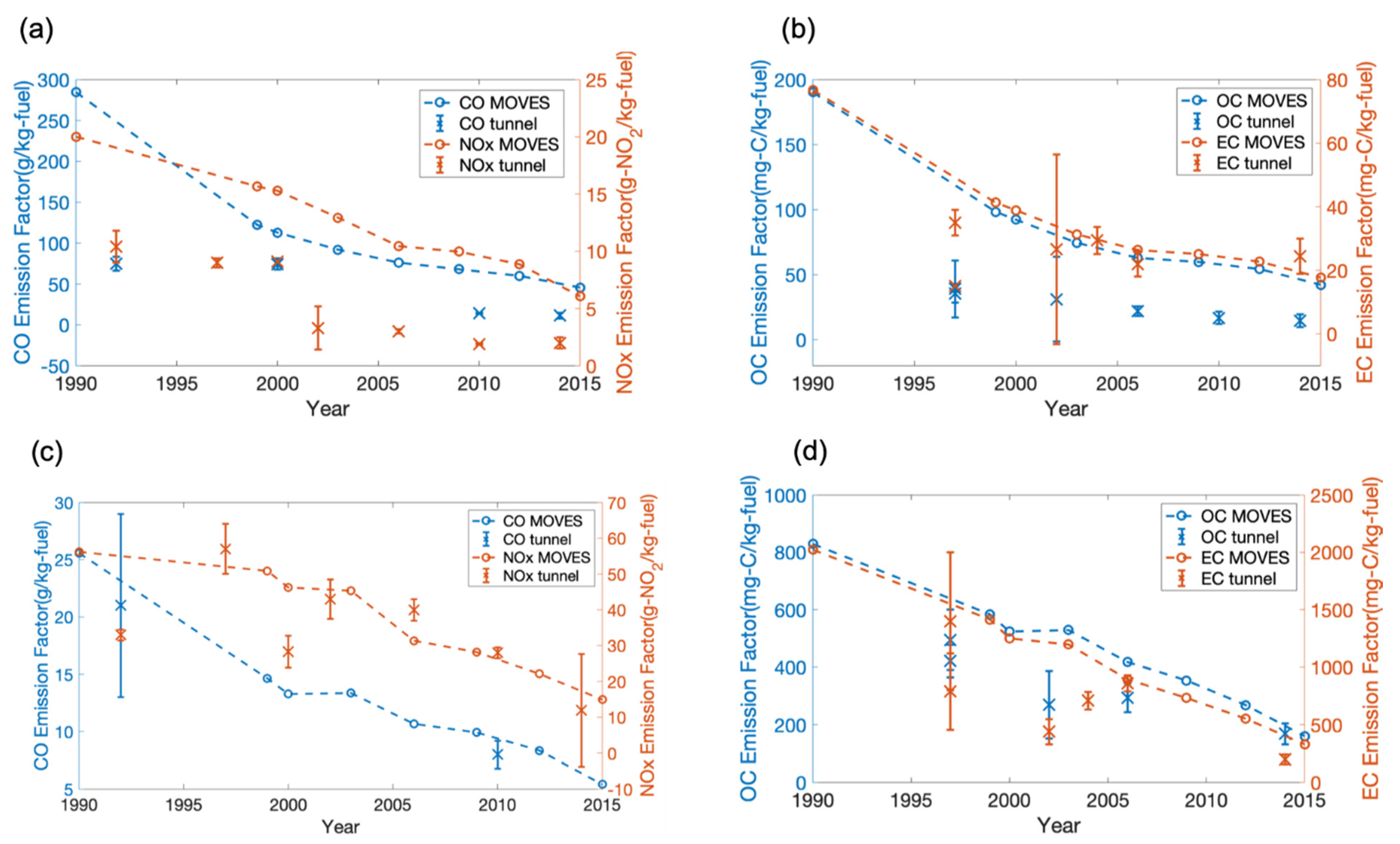
3.4. Long-Term Trend of LDV and HDDV Emission Factors

In a previous section, we compared results from our tunnel measurement with results from Grieshop et al. [14] and concluded that on-road gasoline and diesel vehicle emission factors significantly dropped in the decade between studies. However, this conclusion is based on only two studies in the same city and may not represent the situation over the entire United States. Also, there is significant uncertainty in the diesel emission factors, because we used the regression method in that comparison. Therefore, to further confirm the decreasing trend of on-road vehicle emission factors, we summarized emission factors reported by previous tunnel studies [12,14,26,27,28,29,30,31,32,33] in the United States since the 1990s and compared them with the change of federal vehicle emission standards. The results are presented in Figure 6. All data presented in Figure 6 and the cited previous studies are summarized in Tables S1 and S2.
As shown in Figure 6, over the past three decades, measured LDV and HDDV emission factors decreased as the emission standards became stricter. It indicates that stricter emission standards have been effective at reducing on-road vehicle emissions in the U.S. For example, CO and NOx emission factors for LDV have dropped by 70–80% since 2002. Total PM emissions from LDV have also decreased. This decrease is driven by reductions in OC emissions, whereas EC emissions have been essentially flat. Decreasing LDV emissions of OC and stable EC measured in tunnels echo similar trends observed in dynamometer tests [13,17].
The long-term trend of gas-phase pollutants and PM emitted by HDDV measured in the tunnel are presented in Figure 6c,d, respectively. Tunnel measurements demonstrate a rapid decrease in HDDV NOx emissions associated with 2010 reductions in emissions limits; tunnel studies conducted before 2010 typically measured HDDV NOx emissions >40 g NO2 kg-fuel−1, whereas 2010 data from Dallmann et al. [32] show lower emissions (~30 g NO2 kg-fuel−1), and our data indicate the lowest emissions. Presumably, fleet penetration of SCR for NOx control, which we did not measure directly, increased from 2010 to 2014.
Like NOx in 2010, the HDDV PM emission standard experienced a step change in 2007. Our measurements in 2014 show a significant decrease (~30% decrease) in both EC and OC relative to tunnel studies in the mid-2000s, prior to the introduction of DPFs into the on-road fleet. The introduction of diesel after-treatments has also contributed to reductions in HDDV CO emissions in 2010 and 2014 relative to the 1990s.
Although both LDV and HDDV emission factors measured in tunnels decreased in the past three decades, they did not decrease at the same rate. Thus, the relative significance of HDDV to total on-road vehicle emissions also changed over time. In Table 2 we summarize the ratio of HDDV-to-LDV emission factors measured in previous tunnel studies and in this study in the United States.
The HDDV-to-LDV ratio of NOx emission factors reflects changes in vehicle regulations. Studies in the 1990s observed HDDV/LDV NOx emission ratios in the range of 3–6, and this ratio increased in the mid-2000s to ~13–15, as LDV emissions were reduced relative to HDDV vehicles when Tier-1 and Tier-2 LDV entered the vehicle fleet. Our study is the first among those listed in Table 2 with appreciable penetration of SCR-equipped HDV, and we observed a HDDV/LDV emission ratio of 6, consistent with a rapid drop in HDDV emissions relative to LDV emissions.
HDDV emissions of EC showed a similar rapid drop. The HDDV/LDV EC emission ratio fell by at least 50%, and perhaps more, between the mid-2000s and 2013–2014 when our measurements were acquired. The relative emissions of OC, on the other hand, have been more stable.
In Figure 6, we also compared the vehicle emission factors measured in tunnels with the national level vehicle emission rates simulated by the EPA MOVES. Unlike tunnel studies that only measure the vehicle emissions under high-speed driving, MOVES estimates the vehicle emission factors under a wide range of conditions, including vehicle cold starts and transient operation. The emission factors estimated by MOVES are used for national emission inventory development.
As shown in Figure 6, MOVES consistently has larger estimates for LDV emissions of CO, NOx, and OC than tunnel studies. For 2014, our LDV emission factors for both NOx and CO were roughly half of what is predicted by MOVES. MOVES and the tunnel studies agree better for LDV EC, though for 2014, our measurements suggest a larger EF than MOVES. However, the trend in LDV EC emissions does not agree between MOVES, which shows a smooth decrease with time, and tunnel measurements, which show roughly constant emissions.
Overall, MOVES and the tunnel measurements agree better for HDDV emissions. For HDDV NOx emissions, the tunnel measurements largely agree (within error bounds) with MOVES from 1997 onward. The same is true for CO since 1992, albeit for only three points in time. Agreement for OC and EC is more variable. MOVES predicts higher emissions than tunnel measurements for the 1990s and early 2000s. MOVES also predicts higher emissions than our 2014 data for both OC and EC, though agreement is better than in previous years.

4. Conclusions

In this work, the gaseous and particulate pollutants emitted by on-road gasoline and diesel vehicles under real-world driving conditions were measured in a traffic tunnel. Since the measured fleet average vehicle emission factors are strongly correlated with the % fuelD in the tunnel, we performed linear regression of vehicle emission factors as a function of % fuelD to apportion the gasoline and diesel vehicle emission factors. We found that the NOx and EC emission factors of LDV are about 70% and 40% higher in winter than in spring, respectively.
We compared the emission factors measured in this study with emission factors measured by Greishop et al. [14] ~10 years prior in another traffic tunnel in Pittsburgh and found that the NOx, OC, and EC emission factors of diesel vehicles and the NOx and OC emission factors of gasoline vehicles significantly dropped (~50–70%), while the EC emission factors of gasoline vehicles measured in both studies are similar. To further confirm this long-term trend, we summarized emission factors measured in previous tunnel studies in the U.S. since the 1990s and compared them with the change of vehicle emission standards in U.S. The more restrictive emission standards were effective at reducing NOx and PM emissions of diesel vehicles and NOx, CO, and PM emissions of gasoline vehicles, while the EC emissions of gasoline vehicles did not change much over the past three decades. By studying the trend of HDDV-to-LDV emission factor ratios measured in the tunnel since the 1990s, we found that the relative importance of HDDV for NOx and EC emissions decreased, but the NOx, OC, and EC emissions of HDDV are still significantly higher (~5–10 times) than those of LDV.
The gasoline and diesel vehicle emission factors reported in this study can be used by policy-makers to develop policy plans on regulating air pollutant emissions from on-road vehicles. The application of new vehicle technology, such as the gasoline direct-injection (GDI) engine, coupled with increasingly restrictive emissions standards, may alter the characteristics of vehicle emissions [17,47]. It is therefore necessary to conduct on-road studies to continuously monitor vehicle emissions, test the effectiveness of policies on regulating vehicle emissions, and provide up-to-date vehicle emission factors.

Supplementary Materials

The following are available online at https://0-www-mdpi-com.brum.beds.ac.uk/2076-3417/10/7/2458/s1, Figure S1–S4, Table S1–S2.

Author Contributions

Study design: A.A.P. Measurement and data collection: X.L., T.R.D., A.A.M. Data analysis: X.L., T.R.D. Writing: X.L. and A.A.P. with input from all authors. All authors have read and agreed to the published version of the manuscript.

Funding

X.L. acknowledges a fellowship from the Steinbrenner Institute for Environmental Education and Research.

Conflicts of Interest

The authors declare no conflict of interest.

References

  1. NEI EPA. National Emissions Inventory (NEI). Available online: https://www.epa.gov/air-emissions-inventories (accessed on 15 January 2015).
  2. Dallmann, T.; Harley, R.A. Evaluation of mobile source emission trends in the United States. J. Geophys. Res. Space Phys. 2010, 115, 1–12. [Google Scholar] [CrossRef]
  3. Seinfeld, J.H.; Pandis, S.N. Atmospheric Chemistry and Physics: From Air Pollution to Climate Change, 2nd ed.; John Wiley & Sons: Hoboken, NJ, USA, 2006. [Google Scholar]
  4. Haywood, J.; Boucher, O. Estimates of the direct and indirect radiative forcing due to tropospheric aerosols: A review. Rev. Geophys. 2000, 38, 513–543. [Google Scholar] [CrossRef]
  5. Smith, S.; Bond, T.C. Two hundred fifty years of aerosols and climate: The end of the age of aerosols. Atmos. Chem. Phys. 2014, 14, 537–549. [Google Scholar] [CrossRef] [Green Version]
  6. Di, Q.; Wang, Y.; Zanobetti, A.; Wang, Y.; Koutrakis, P.; Choirat, C.; Dominici, F.; Schwartz, J.D. Air Pollution and Mortality in the Medicare Population. N. Engl. J. Med. 2017, 376, 2513–2522. [Google Scholar] [CrossRef] [PubMed]
  7. Dockery, D.W.; Pope, C.A.; Xu, X.; Spengler, J.D.; Ware, J.H.; Fay, M.E.; Ferris, B.G.; Speizer, F.E. An Association between Air Pollution and Mortality in Six U.S. Cities. N. Engl. J. Med. 1993, 329, 1753–1759. [Google Scholar] [CrossRef] [Green Version]
  8. Kanakidou, M.; Seinfeld, J.H.; Pandis, S.; Barnes, I.; Dentener, F.J.; Facchini, M.C.; Van Dingenen, R.; Ervens, B.; Nenes, A.; Nielsen, C.J.; et al. Organic aerosol and global climate modelling: A review. Atmos. Chem. Phys. 2005, 5, 1053–1123. [Google Scholar] [CrossRef] [Green Version]
  9. Zhang, Q.; Jimenez, J.-L.; Canagaratna, M.R.; Allan, J.D.; Coe, H.; Ulbrich, I.; Alfarra, M.R.; Takami, A.; Middlebrook, A.; Sun, Y.; et al. Ubiquity and dominance of oxygenated species in organic aerosols in anthropogenically-influenced Northern Hemisphere midlatitudes. Geophys. Res. Lett. 2007, 34, 34. [Google Scholar] [CrossRef] [Green Version]
  10. Maricq, M.M. Chemical characterization of particulate emissions from diesel engines: A review. J. Aerosol Sci. 2007, 38, 1079–1118. [Google Scholar] [CrossRef]
  11. Turns, S.R. An Introduction to Combustion: Concepts and Applications; McGraw-Hill: New York, NY, USA, 2000; Volume 499. [Google Scholar]
  12. Kirchstetter, T.W.; Harley, R.A.; Kreisberg, N.M.; Stolzenburg, M.R.; Hering, S.V. On-road measurement of fine particle and nitrogen oxide emissions from light- and heavy-duty motor vehicles. Atmos. Environ. 1999, 33, 2955–2968. [Google Scholar] [CrossRef]
  13. May, A.A.; Nguyen, N.T.; Presto, A.; Gordon, T.; Lipsky, E.; Karve, M.; Gutierrez, A.; Robertson, W.H.; Zhang, M.; Brandow, C.; et al. Gas- and particle-phase primary emissions from in-use, on-road gasoline and diesel vehicles. Atmos. Environ. 2014, 88, 247–260. [Google Scholar] [CrossRef]
  14. Grieshop, A.; Lipsky, E.; Pekney, N.J.; Takahama, S.; Robinson, A. Fine particle emission factors from vehicles in a highway tunnel: Effects of fleet composition and season. Atmos. Environ. 2006, 40, 287–298. [Google Scholar] [CrossRef]
  15. Li, X.; Dallmann, T.R.; May, A.A.; Stanier, C.O.; Grieshop, A.; Lipsky, E.; Robinson, A.; Presto, A. Size distribution of vehicle emitted primary particles measured in a traffic tunnel. Atmos. Environ. 2018, 191, 9–18. [Google Scholar] [CrossRef]
  16. Nam, E.; Kishan, S.; Baldauf, R.W.; Fulper, C.R.; Sabisch, M.; Warila, J. Temperature Effects on Particulate Matter Emissions from Light-Duty, Gasoline-Powered Motor Vehicles. Environ. Sci. Technol. 2010, 44, 4672–4677. [Google Scholar] [CrossRef] [PubMed]
  17. Saliba, G.; Saleh, R.; Zhao, Y.; Presto, A.; Lambe, A.T.; Frodin, B.; Sardar, S.; Maldonado, H.; Maddox, C.; May, A.A.; et al. Comparison of Gasoline Direct-Injection (GDI) and Port Fuel Injection (PFI) Vehicle Emissions: Emission Certification Standards, Cold-Start, Secondary Organic Aerosol Formation Potential, and Potential Climate Impacts. Environ. Sci. Technol. 2017, 51, 6542–6552. [Google Scholar] [CrossRef] [PubMed]
  18. Gouriou, F.; Morin, J.-P.; Weill, M.-E. On-road measurements of particle number concentrations and size distributions in urban and tunnel environments. Atmos. Environ. 2004, 38, 2831–2840. [Google Scholar] [CrossRef]
  19. Durant, J.; Ash, C.A.; Wood, E.C.; Herndon, S.C.; Jayne, J.; Knighton, W.B.; Canagaratna, M.R.; Trull, J.B.; Brügge, D.; Zamore, W.; et al. Short-term variation in near-highway air pollutant gradients on a winter morning. Atmos. Chem. Phys. 2010, 10, 8341–8352. [Google Scholar] [CrossRef] [Green Version]
  20. Kam, W.; Liacos, J.W.; Schauer, J.J.; Delfino, R.J.; Sioutas, C. On-road emission factors of PM pollutants for light-duty vehicles (LDVs) based on urban street driving conditions. Atmos. Environ. 2012, 61, 378–386. [Google Scholar] [CrossRef]
  21. Zhu, Y.; Hinds, W.C.; Kim, S.; Shen, S.; Sioutas, C. Study of ultrafine particles near a major highway with heavy-duty diesel traffic. Atmos. Environ. 2002, 36, 4323–4335. [Google Scholar] [CrossRef]
  22. Saha, P.K.; Khlystov, A.; Snyder, M.G.; Grieshop, A. Characterization of air pollutant concentrations, fleet emission factors, and dispersion near a North Carolina interstate freeway across two seasons. Atmos. Environ. 2018, 177, 143–153. [Google Scholar] [CrossRef]
  23. Liggio, J.; Gordon, M.; Smallwood, G.; Li, S.-M.; Stroud, C.; Staebler, R.; Lu, G.; Lee, P.; Taylor, B.; Brook, J.R. Are Emissions of Black Carbon from Gasoline Vehicles Underestimated? Insights from Near and On-Road Measurements. Environ. Sci. Technol. 2012, 46, 4819–4828. [Google Scholar] [CrossRef]
  24. Canagaratna, M.R.; Jayne, J.T.; Ghertner, D.A.; Herndon, S.; Shi, Q.; Jimenez, J.-L.; Silva, P.J.; Williams, P.; Lanni, T.; Drewnick, F.; et al. Chase Studies of Particulate Emissions from in-use New York City Vehicles. Aerosol Sci. Technol. 2004, 38, 555–557. [Google Scholar] [CrossRef]
  25. Massoli, P.; Fortner, E.C.; Canagaratna, M.R.; Williams, L.R.; Zhang, Q.; Sun, Y.; Schwab, J.J.; Trimborn, A.; Onasch, T.B.; Demerjian, K.L.; et al. Pollution Gradients and Chemical Characterization of Particulate Matter from Vehicular Traffic near Major Roadways: Results from the 2009 Queens College Air Quality Study in NYC. Aerosol Sci. Technol. 2012, 46, 1201–1218. [Google Scholar] [CrossRef]
  26. Ban-Weiss, G.; McLaughlin, J.P.; Harley, R.A.; Lunden, M.M.; Kirchstetter, T.W.; Kean, A.J.; Strawa, A.W.; Stevenson, E.D.; Kendall, G.R. Long-term changes in emissions of nitrogen oxides and particulate matter from on-road gasoline and diesel vehicles. Atmos. Environ. 2008, 42, 220–232. [Google Scholar] [CrossRef]
  27. Pierson, W.R.; Gertler, A.W.; Robinson, N.F.; Sagebiel, J.C.; Zielinska, B.; Bishop, G.; Stedman, D.H.; Zweidinger, R.B.; Ray, W.D. Real-world automotive emissions—Summary of studies in the Fort McHenry and Tuscarora mountain tunnels. Atmos. Environ. 1996, 30, 2233–2256. [Google Scholar] [CrossRef]
  28. Miguel, A.H.; Kirchstetter, T.W.; Harley, R.A.; Hering, S.V. On-Road Emissions of Particulate Polycyclic Aromatic Hydrocarbons and Black Carbon from Gasoline and Diesel Vehicles. Environ. Sci. Technol. 1998, 32, 450–455. [Google Scholar] [CrossRef]
  29. Allen, J.O.; Mayo, P.R.; Hughes, L.S.; Salmon, L.G.; Cass, G.R. Emissions of size-segregated aerosols from on-road vehicles in the Caldecott tunnel. Environ. Sci. Technol. 2001, 35, 4189–4197. [Google Scholar] [CrossRef]
  30. McGaughey, G.R.; Desai, N.R.; Allen, D.T.; Seila, R.L.; Lonneman, W.A.; Fraser, M.P.; Harley, R.A.; Pollack, A.K.; Ivy, J.M.; Price, J.H. Analysis of motor vehicle emissions in a Houston tunnel during the Texas Air Quality Study 2000. Atmos. Environ. 2004, 38, 3363–3372. [Google Scholar] [CrossRef]
  31. Geller, M.D.; Sardar, S.B.; Phuleria, H.; Fine, P.M.; Sioutas, C. Measurements of Particle Number and Mass Concentrations and Size Distributions in a Tunnel Environment. Environ. Sci. Technol. 2005, 39, 8653–8663. [Google Scholar] [CrossRef]
  32. Dallmann, T.; DeMartini, S.J.; Kirchstetter, T.W.; Herndon, S.C.; Onasch, T.B.; Wood, E.C.; Harley, R.A. On-Road Measurement of Gas and Particle Phase Pollutant Emission Factors for Individual Heavy-Duty Diesel Trucks. Environ. Sci. Technol. 2012, 46, 8511–8518. [Google Scholar] [CrossRef]
  33. Dallmann, T.; Kirchstetter, T.W.; DeMartini, S.J.; Harley, R.A. Quantifying On-Road Emissions from Gasoline-Powered Motor Vehicles: Accounting for the Presence of Medium- and Heavy-Duty Diesel Trucks. Environ. Sci. Technol. 2013, 47, 13873–13881. [Google Scholar] [CrossRef]
  34. Misra, C.; Collins, J.F.; Herner, J.D.; Sax, T.; Krishnamurthy, M.; Sobieralski, W.; Burntizki, M.; Chernich, D. In-Use NOx Emissions from Model Year 2010 and 2011 Heavy-Duty Diesel Engines Equipped with Aftertreatment Devices. Environ. Sci. Technol. 2013, 47, 7892–7898. [Google Scholar] [CrossRef]
  35. Bishop, G.; Haugen, M. The Story of Ever Diminishing Vehicle Tailpipe Emissions as Observed in the Chicago, Illinois Area. Environ. Sci. Technol. 2018, 52, 7587–7593. [Google Scholar] [CrossRef] [PubMed]
  36. Wang, J.M.; Jeong, C.-H.; Zimmerman, N.; Healy, R.; Evans, G.J. Real world vehicle fleet emission factors: Seasonal and diurnal variations in traffic related air pollutants. Atmos. Environ. 2018, 184, 77–86. [Google Scholar] [CrossRef]
  37. Grange, S.K.; Farren, N.J.; Vaughan, A.R.; Rose, R.A.; Carslaw, D.C. Strong Temperature Dependence for Light-Duty Diesel Vehicle NOx Emissions. Environ. Sci. Technol. 2019, 53, 6587–6596. [Google Scholar] [CrossRef] [PubMed] [Green Version]
  38. US Environmental Protection Agency. MOVES2014a User Guide; US Environmental Protection Agency: Washington, DC, USA, 2015.
  39. California Air Resources Board. EMFAC2017 User’s Guide; California Air Resources Board: Sacramento, CA, USA, 2017.
  40. Li, X.; Dallmann, T.R.; May, A.A.; Tkacik, D.S.; Lambe, A.T.; Jayne, J.T.; Croteau, P.L.; Presto, A. Gas-Particle Partitioning of Vehicle Emitted Primary Organic Aerosol Measured in a Traffic Tunnel. Environ. Sci. Technol. 2016, 50, 12146–12155. [Google Scholar] [CrossRef]
  41. Tkacik, D.S.; Lambe, A.T.; Jathar, S.H.; Li, X.; Presto, A.; Zhao, Y.; Blake, D.R.; Meinardi, S.; Jayne, J.T.; Croteau, P.L.; et al. Secondary Organic Aerosol Formation from in-Use Motor Vehicle Emissions Using a Potential Aerosol Mass Reactor. Environ. Sci. Technol. 2014, 48, 11235–11242. [Google Scholar] [CrossRef] [Green Version]
  42. United States Department of Transportation. National Transportation Statistics. Available online: www.rita.dot.gov/bts/sites/rita.dot.gov.bts/files/publications/national_transportation_statistics/index.html (accessed on 15 January 2015).
  43. Gertler, A.W.; Gillies, J.A.; Pierson, W.R.; Rogers, C.F.; Sagebiel, J.C.; Abu-Allaban, M.; Coulombe, W.; Tarnay, L.; Cahill, T.A. Real-world particulate matter and gaseous emissions from motor vehicles in a highway tunnel. Res. Rep. (Health Eff. Inst.) 2002, 107, 5–56. [Google Scholar]
  44. Fraser, M.P.; Buzcu, B.; Yue, Z.W.; McGaughey, G.R.; Desai, N.R.; Allen, D.T.; Seila, R.L.; Lonneman, W.A.; Harley, R.A. Separation of Fine Particulate Matter Emitted from Gasoline and Diesel Vehicles Using Chemical Mass Balancing Techniques. Environ. Sci. Technol. 2003, 37, 3904–3909. [Google Scholar] [CrossRef]
  45. May, A.A.; Presto, A.; Hennigan, C.; Nguyen, N.T.; Gordon, T.; Robinson, A. Gas-Particle Partitioning of Primary Organic Aerosol Emissions: (2) Diesel Vehicles. Environ. Sci. Technol. 2013, 47, 8288–8296. [Google Scholar] [CrossRef]
  46. May, A.A.; Presto, A.; Hennigan, C.; Nguyen, N.T.; Gordon, T.; Robinson, A. Gas-particle partitioning of primary organic aerosol emissions: (1) Gasoline vehicle exhaust. Atmos. Environ. 2013, 77, 128–139. [Google Scholar] [CrossRef]
  47. Zimmerman, N.; Wang, J.M.; Jeong, C.-H.; Wallace, J.S.; Evans, G.J. Assessing the Climate Trade-Offs of Gasoline Direct Injection Engines. Environ. Sci. Technol. 2016, 50, 8385–8392. [Google Scholar] [CrossRef] [PubMed] [Green Version]
Figure 1. Background fraction of pollutants measured in the tunnel in the spring campaign. OC: organic carbon, EC: elemental carbon.
Applsci 10 02458 g001
Figure 2. Diurnal patterns of the hourly averaged (a) NOx, (b) OC, (c) EC, and (d) CO emission factors measured in the tunnel on weekdays in spring (right axis) and the heavy-duty diesel vehicle (HDDV) fuel fraction (left axis). Bars represent the standard deviation of the measurement. OC and EC data are not available at 04:00 and 05:00 because the instrument ran a blank sample each day in that period. R2 values show the correlation between hourly averaged % fuelD and emission factor.
Applsci 10 02458 g002
Figure 3. The (a) NOx, (b) OC, and (c) EC emission factors as a function of % fuelD over the % fuelD range of 0–0.4. Circles represent measurement data, and the color represents the average ambient temperature during the measurement. The linear regression lines of spring and winter measurements are shown as red and green lines, respectively. Red and green shadings are the simultaneous functional bounds of the linear fit at the 95% confidence level for spring and winter measurements, respectively.
Applsci 10 02458 g003
Figure 4. The (a) weekday and (b) weekend diurnal profiles of CO emission factors measured in the Fort Pitt Tunnel in winter and spring.
Applsci 10 02458 g004
Figure 5. The (a) NOx, (b) OC, and (c) EC emission factors as a function of % fuelD over the % fuelD range of 0–1. The linear regression lines of spring and winter measurements are shown as red and green lines, respectively. Black dashed lines are linear regression results of Grieshop et al [14]. Symbols with error bars represent mean values and standard deviations measured in recent dynamometer studies by May et al [13].
Applsci 10 02458 g005
Figure 6. Emission factors of (a) gaseous pollutants emitted by LDV, (b) particulate pollutants emitted by LDV, (c) gaseous pollutants emitted by HDDV, and (d) particulate pollutants emitted by HDDV measured in tunnels in the United States since the 1990s. The emission factors of LDV and HDDV simulated by EPA MOtor Vehicle Emission Simulator (MOVES) are also presented in the figure as dashed lines. The data and cited previous studies of emission factors are summarized in Table S1 (LDV) and Table S2 (HDDV). For CO emission factors in 2014, we used the average winter emission factors from this study. For emission factors measured in 1992 and reported by Pierson et al., only the uphill measurements conducted in the Fort McHenry Tunnel are shown.
Applsci 10 02458 g006
Table 1. Mean emission factors of light-duty gasoline vehicles (LDV) and heavy-duty diesel vehicles (HDDV) measured in the Fort Pitt Tunnel. SCR: selective catalytic reduction, DPF: diesel particulate filter.
Species (Emission Factor Units)Vehicle TypeSpring RegressionWinter RegressionDynamometer
(May et al.)
NOx (g NO2/kg fuel)LDV1.2 ± 0.32 ± 0.52.7
HDDV17.1 ± 2.429.2 ± 3.218.2 (no SCR)
s5.2 (with SCR)
OC (mg/kg fuel)LDV18.5 ± 7.214.7 ± 4.811.3
HDDV109.4 ± 54.0167.8 ± 36.3117.0 (no DPF)
7.6 (with DPF)
EC (mg/kg fuel)LDV15.9 ± 4.524.4 ± 5.517.2
HDDV158.7 ± 33.8196.8 ± 41.1182.8 (no DPF)
0.3 (with DPF)
Table 2. Ratio of HDDV-to-LDV emission factors measured in traffic tunnels in the United States.
ReferencesTunnelYear of MeasurementNOxOCEC
Pierson et al.Fort McHenry Tunnel, MD, Downhill19924.0 ± 0.4 a--
Pierson et al.Fort McHenry Tunnel, MD, uphill19923.2 ± 0.5 a--
Pierson et al.Tuscarora Mountain Tunnel, PA, level19926.9 ± 5.0 a--
Miguel et al.Caldecott Tunnel, CA1996---
Kirchstetter et al.Caldecott Tunnel, CA19976.3 ± 0.8 b11.8 ± 2.8 b,c40.0 ± 17.7 b
Allen et al.Caldecott Tunnel, CA1997-12.7 ± 7.6 d52.5 ± 249.6 d
McGaughey et al.Washburn Tunnel, TX20003.1 ± 5.1 e--
Gëller et al.Caldecott Tunnel, CA2004--24.1 ± 4.4 f
Grieshop et al.Squirrel Hill Tunnel, PA2002 and 200413.0 ± 7.78.6 ± 9.716.5 ± 18.9
Ban-Weiss et al.Caldecott Tunnel, CA200613.3 ± 1.313.3 ± 3.1 g39.1 ± 7.8
Dallmann et al.Caldecott Tunnel, CA201014.7 ± 1.0 h--
This workFort Pitt Tunnel, PA2013–20146.0 ± 8.011.4 ± 4.58.1 ± 2.5
a We assumed one gallon of gasoline weighs 2.80 kg and one gallon of diesel weighs 3.24 kg to convert units. b Data calculated by Ban-Weiss et al. using the revised regression method are reported here. c A factor of 1.4 was used to convert Organic Matter (OM) concentration to OC concentration. d Data reported here are for PM1.9. e We assumed the carbon fraction of diesel equals to 0.87 to convert units. We assumed the density of gasoline equals to 0.74 kg/L to convert units. The diesel vehicle emission factors reported here are calculated based on the linear regression results from Table 4 of McCaughey et al. f Data reported here are for PM2.5. g A factor of 1.4 was used to convert OM concentration to OC concentration. h We used adjusted light-duty-vehicle emission factors reported in Dallmann et al. as the LDV emission factor to calculate these ratios.

