Calibration and Image Reconstruction in a Spot Scanning Detection System for Surface Defects

1
State Key Laboratory of Modern Optical Instrumentation, Department of Optical Engineering, Zhejiang University, 38 Zheda Road, Hangzhou 310027, China
2
Zernike Optics Co., Ltd., 10 Shengang Road, Hangzhou 310027, China
*
Author to whom correspondence should be addressed.
Appl. Sci. 2020, 10(7), 2503; https://0-doi-org.brum.beds.ac.uk/10.3390/app10072503
Submission received: 27 February 2020
/
Revised: 2 April 2020
/
Accepted: 3 April 2020
/
Published: 5 April 2020
Abstract
:Compared to traditional approaches, the spot scanning surface defect evaluation system (SS-SDES) has better performances on the detection of small defects and defect classification for optical surfaces. However, the existing system deviations will cause distortions and even a missing area in the defect image which is reconstructed from the acquired raw data based on the scanning trace, thus degrading the reliability of detection results. To solve these problems, a system calibration method is proposed with the parameterization of these deviations and the modeling of practical scanning trace. A constraint function, to characterize the straightness and scale errors in the image, is defined. Then an optimization is implemented to minimize it and hence to obtain the optimal estimate of the system deviations, which is subsequently used to adjust the system and reconstruct reliable defect images. Additionally, to further enhance the image quality, an image reconstruction method capable of suppressing signal noise through a weighted average strategy is proposed. Experiments show that with our methods, the system deviations are effectively corrected, and a complete and precise defect image with low distortions that are within 1.8 pixels is reconstructed. Therefore, the detection accuracy and reliability of the system can be improved.
1. Introduction
The detection of surface defects is one of the main items of surface quality evaluation for optical elements. In optical systems, scattering induced by surface defects will reduce the utilization efficiency of energy or even lead to severe damage to those with high-energy lasers, such as the inertial confinement fusion system (ICF) [1,2,3]. With the wide application of the optical elements and the development of manufacturing technology, the requirements for defect detection become higher. On the one hand, sufficient detection sensitivity for small-size defects is required to ensure the effectiveness and safety of optical elements for use. On the other hand, to obtain a comprehensive evaluation report containing hazard assessment and cause analysis of defects, the ability of quantitative detection, including defect size metrology and defect classification, has become increasingly significant.
Various detection approaches for surface defects of optical elements have been studied. Commercial microscopes, such as atomic force microscope (AFM) and scanning electron microscope (SEM), are used to detect and characterize the surface defects on fine optics [4,5]. These methods have high detection accuracy and sensitivity but require long inspection times. Because of the advantages of non-destructiveness and high throughput, optical inspection techniques have gained more and more attention. For example, Choi et al. [6] proposed a defect inspection method which obtains defect images using the photo-thermal reflectance technique. Rainer et al. [7] adopt the total internal reflection (TIR) technique with back and edge illuminations to detect both the surface defects and sub-surface damages of large optical elements. At present, the most common detection approaches for surface defects are based on the dark-field scattering technique [8,9,10]. On this basis, a surface defect evaluation system (SDES) has been proposed and established from our previous works [11,12,13]. It employs subaperture scanning, image stitching, and image processing methods to finally realize the quantitative inspection of surface defects down to micrometer-level dimension. The measuring aperture can reach the order of a meter. However, because the SDES uses a zoom microscope with a long working distance, the numerical aperture of the objective is relatively low. As a result, only a small amount of scattered light induced by defects can be collected, and therefore, especially for small-size defects (such as shallow scratches), the defect signal acquired by the image sensor will be weak [14]. Hence, the detection sensitivity is limited. Moreover, the SDES lacks the ability to distinguish the defects that exhibit similar features in the acquired image [15].
In detection approaches based on dark-field scattering techniques, enhancing the defect scattering signal is an effective way to improve the detection sensitivity [16]. For this purpose, a spot scanning surface defect evaluation system (SS-SDES) is established in this paper. A short-wavelength laser beam is focused on the optical surface to form an illuminated spot, and a positioning system is used to bring the spot onto each portion of the surface along a spiral trace. In each illuminated spot, the scattered light caused by defects will be collected by a large solid-angle ellipsoidal mirror, and then detected by a high-sensitivity photomultiplier (PMT), thus improving the intensity of the acquired defect scattering signal. Additionally, the SS-SDES incorporates a polarization measurement channel, which is capable of measuring the polarization characterization of defects for classification. Due to the use of the spot scanning technique, the SS-SDES cannot, like an image sensor-based system, acquire a defect image directly. Therefore, before defect extraction and analysis, the SS-SDES needs to perform image reconstruction on the acquired intensity signals. However, the existing system deviations, such as the position deviation of the illuminated spot, will cause distortions and even a missing area in the reconstructed image, which will affect the detection results in many aspects and hence degrade the reliability of the system. Although there have been several studies on distortion correction [17,18], they are mostly aimed at the optical distortion caused by imaging lenses and cameras, so they are not applicable to the situation in this paper.
To address these issues, this paper develops a system calibration method based on straightness and scale constraints and an image reconstruction method based on weighted average. First, the system deviations are parameterized to model the practical scanning trace, which will be used to compute the image coordinate of each acquired intensity signal. On this basis, a calibration plate with specific defect patterns is employed as the test sample, and several constraints are established to constrain the image coordinates corresponding to these defects. Then, an optimization is implemented to minimize the constraints and hence to obtain the optimal estimate of the system deviations. This estimate is subsequently used to adjust the system and establish an accurate mapping relationship for image reconstruction. The adjusted system can perform the scan for the whole optical surface in a normal way but without any missing area. Finally, using the proposed image reconstruction method, a complete defect image with low noise and low distortion can be obtained; this will greatly improve the detection accuracy and reliability of the system. The proposed methods are applicable to any other detection systems based on spot scanning, such as those for wafers, films, and rough surfaces.
The remainder of this paper is as follows. Section 2 introduces the configuration of the SS-SDES and the ideal image reconstruction and then summarizes the existing system deviations as well as their impacts. In Section 3, the modeling of practical scanning trace and the details of the proposed system calibration method and image reconstruction method are described. Section 4 shows the experiment and comparison results, and Section 5 presents a conclusion of this paper.
2. Spot Scanning Surface Defect Evaluation System
2.1. System Layout
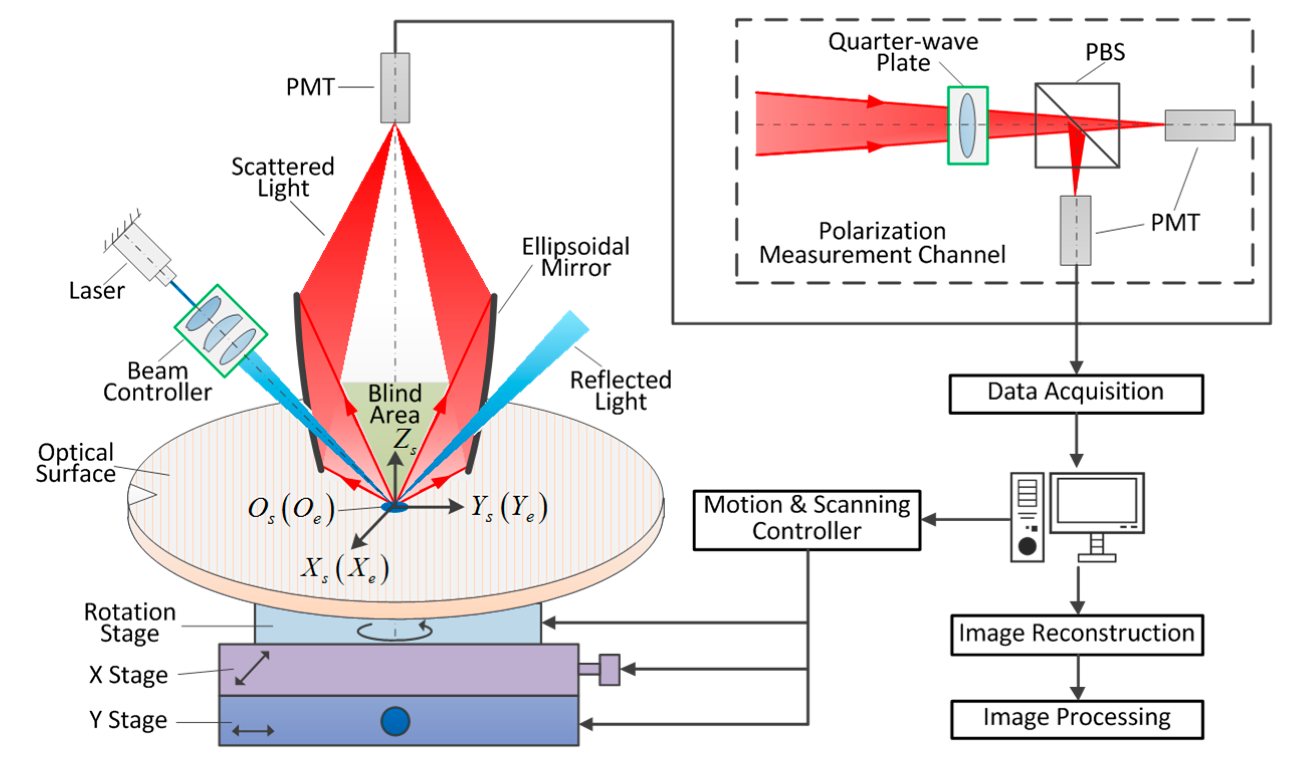
Figure 1 presents the system layout of the SS-SDES. A short-wavelength laser beam passes through a beam controller to obtain a specific polarization state and is subsequently focused onto the optical surface to be inspected. If there is no defect in the illuminated spot, the light will be specularly reflected by the optical surface. Otherwise, the defects will produce scattered light in all directions. An ellipsoidal mirror is used to collect the scattered light beams with a large solid angle and reflects them into a photomultiplier (PMT) for detection. The basic principle is that each beam of light that passes through a focal point of the ellipsoidal mirror will pass through another focal point after being reflected. Thus, the ellipsoidal mirror is properly placed, making its two focal points coincide with the illuminated spot and the PMT, respectively. The reflected light is led through a hole in the mirror to escape so that the scattered light is detected only. Such an optical configuration can greatly enhance the acquired scattering signal of defects while keeping the background signal at a normal level, thus offering the potential to detect smaller-size defects to the system. The SS-SDES incorporates a polarization measurement channel as well. The scattered light in the blind area of the mirror is led into this channel, where a quarter-wave plate and a polarization beam splitter (PBS) are exploited to separate the light into two beams according to its polarization state. Both of them are finally detected by two additional PMTs, respectively, forming a two-dimensional polarization signal for further defect classification [19,20].
To realize a scan for the whole surface, the optical sample is placed on a positioning system, which includes a rotation stage and a two-dimensional translation stage. Under the control of a computer, the positioning system rotates and translates the sample, allowing the whole surface to be scanned along a spiral trace. And the intensity signals detected by the PMTs are synchronously acquired and recorded using a data acquisition card with a specific sampling frequency. Based on the scanning trace, image reconstruction is performed on the acquired signal sequence to obtain defect images. With those, a quantitative evaluation for surface defects can be finally achieved after further image processing and analysis.
2.2. Ideal Scanning Trace and Image Reconstruction
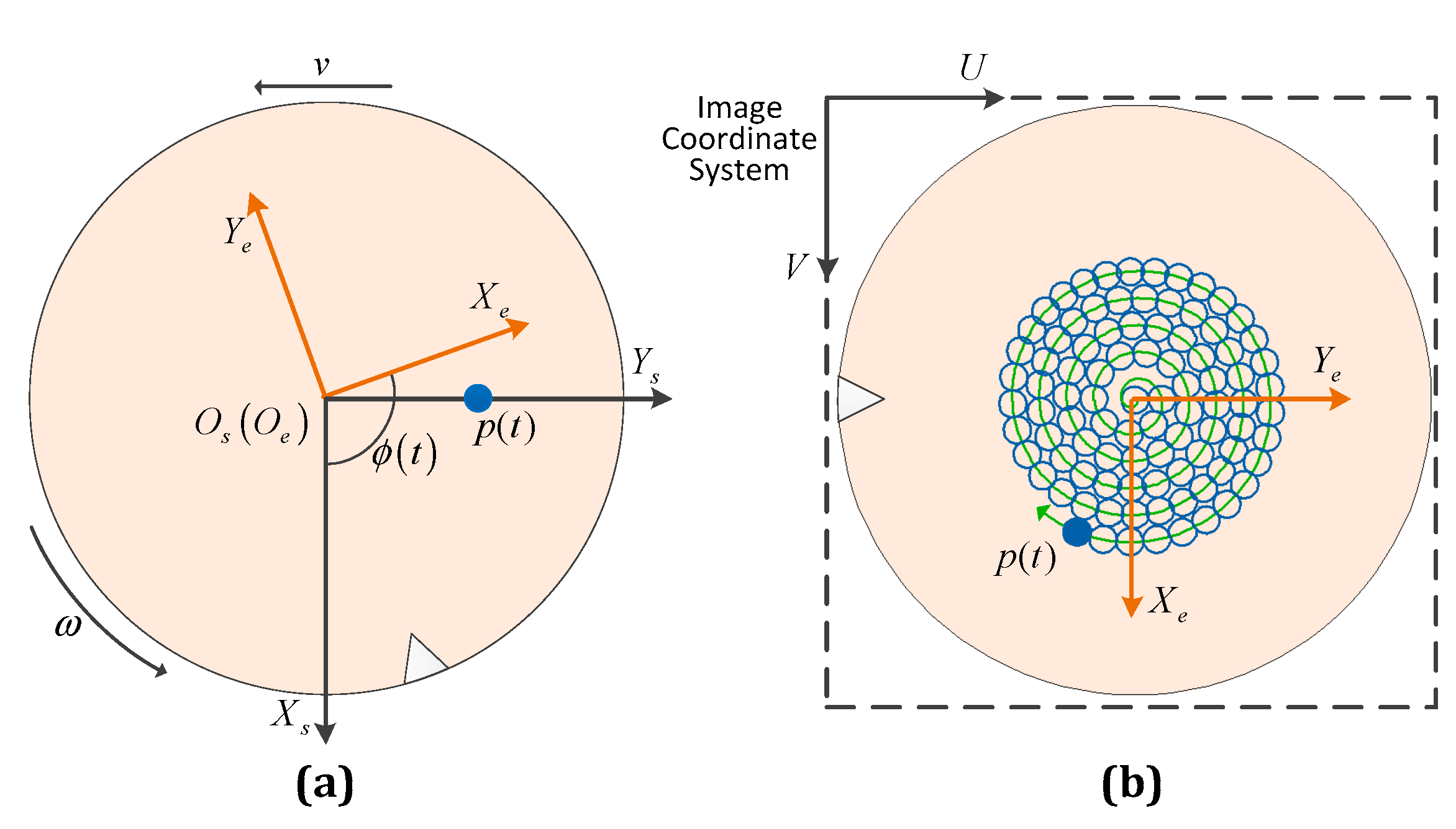
Two coordinate systems need to be established for the analysis of scanning trace and image reconstruction. The first one is the three-dimensional system coordinate system , as shown in Figure 1, which takes the horizontal two-dimensional translation stage as the x-axis and the y-axis, the vertical up as the z-axis, and the intersection of the axis of the rotation stage (the rotation axis) and the optical surface as the origin. The second one is the two-dimensional surface coordinate system . It coincides with at the initial system state (that is, both the rotation stage and the two-dimensional translation stage are at their own original positions). During scanning, both of them will move under the driving of the positioning system, and the surface coordinate system will also rotate as the optical surface does. Ideally, the rotation axis coincides with the axis, and the illuminated spot at the initial system state (called the initial illuminated spot) is at point . Figure 2 illustrates the scanning diagram of the system under ideal conditions. The positioning system translates along the negative direction of the axis at a constant velocity of and rotates counterclockwise at an angular velocity of . At any scanning time , as shown in Figure 2a, the coordinate of the illuminated spot in the system coordinate system is , and the rotation angle of the surface coordinate system relative to the system coordinate system is , where represents the number of revolutions that have been rotated. Hence, the coordinate of in the surface coordinate system, , can be calculated by rotation transformation as
The intensity signals detected by each PMT are acquired and recorded with a sampling frequency of , forming a discrete intensity sequence , where is the total number of sampling points. Figure 2b presents the spiral scanning trace and the distribution of sampling points. For each sampling point in the sequence, the corresponding scanning time depends on its sequence number , as , and the corresponding intensity signal is . By using Equation (1), the coordinate of the sampling point in the surface coordinate system can be obtained, which is subsequently converted to the image coordinate in the reconstructed image by
where is the image coordinate of the first sampling point with , which needs to be preset according to the actual scanning range to ensure that the image coordinates of all sampling points are positive; the coefficient represents the actual size of each pixel. In the SS-SDES, the value of is equal to the translation distance of the positioning system by a single revolution, defined as . Combined with the derived image coordinates and corresponding intensity signals, a complete defect image can be reconstructed.
2.3. Deviations in the System and their Consequences
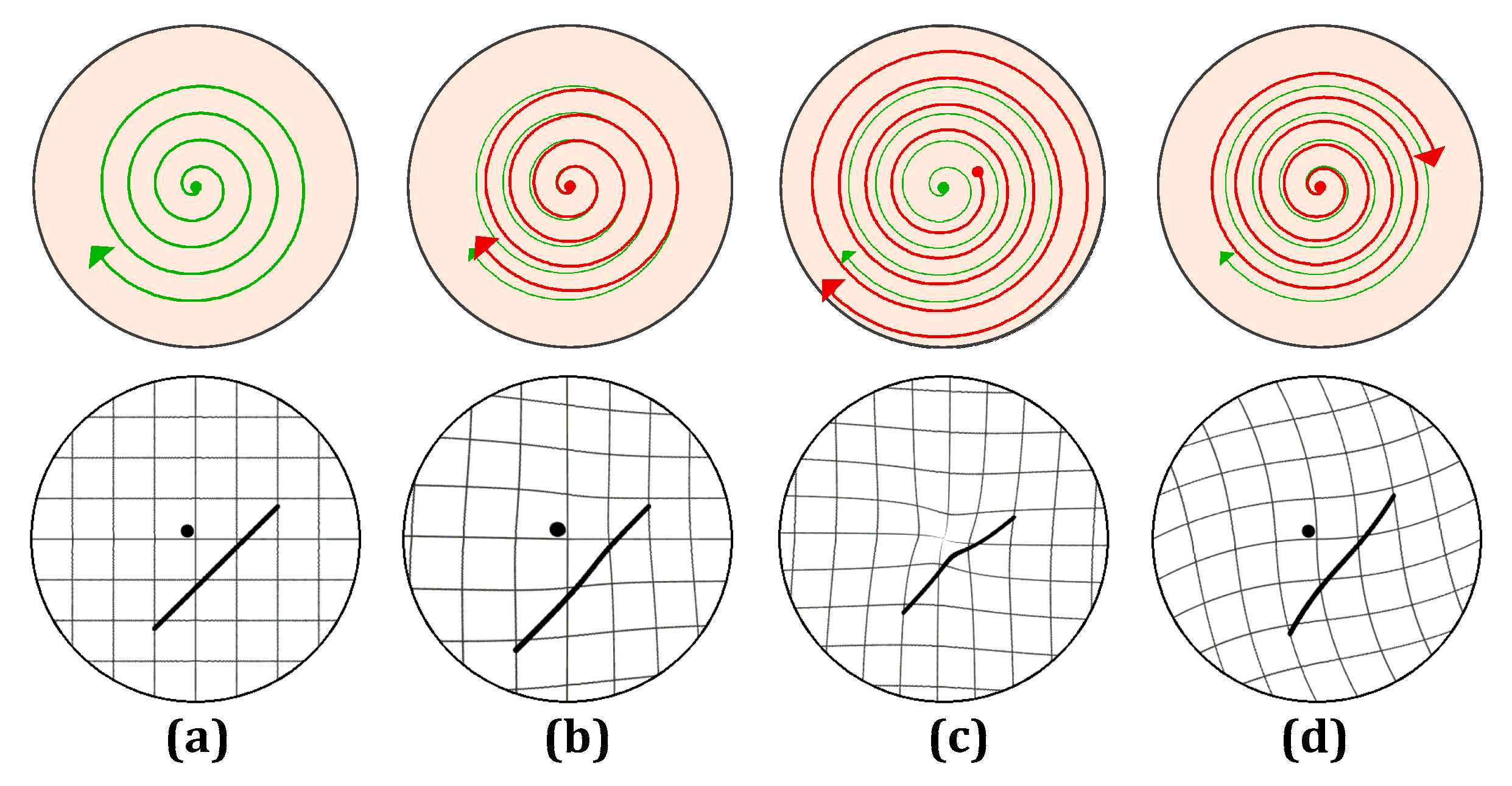
However, the practical scanning trace will differ from the ideal scanning trace due to the existence of system deviations, including the following: (1) angle deviation of the rotation axis from the axis; (2) position deviation of the initial illuminated spot from the origin ; and (3) deviations of translation velocity, rotation velocity, and sampling frequency from their setting values. Because the optical sample is precisely leveled when it is placed, the surface can be considered as a horizontal plane at the initial system state. In this case, if the ideal scanning trace is still used for image reconstruction, distortions will be introduced. This section will simulate the impacts of these system deviations on the scanning trace and image reconstruction. The specific models involved in the simulation will be given in the next section.
Figure 3 presents the simulated practical scanning traces (upper row) and the corresponding images (lower row) reconstructed using the ideal scanning trace, where a–d represent the cases with no deviation, angle deviation of the rotation axis, position deviation of the initial illuminated spot, and rotation velocity deviation, respectively. It can be seen that these system deviations can change the scanning traces to some degree and hence yield obvious distortions in the reconstructed images. The distortions will affect the accuracy of detection results in many aspects, such as causing the displacement of the defect’s location and the scaling of the defect’s size. Line-like defects, such as scratches, may appear bent, leading to an inaccurate extraction of the curvature features. Moreover, the position deviation of the initial illuminated spot will even produce an undetected area that is not scanned at the center of the surface. As shown in Figure 3c, the consequence of this issue is that the point-like defect near the center in the reconstructed image is missing. According to the analysis, the existence of system deviations will severely reduce the reliability of the SS-SDES. It is significant to propose an effective and accurate method for system calibration and image reconstruction.
3. System Calibration and Image Reconstruction Methods
To address the problems introduced by system deviations, this paper proposes a novel system calibration method based on straightness and scale constraints and an image reconstruction method based on weighted average. The methods will be described in detail below, including the following: (1) how to parameterize the system deviations and model the practical scanning trace; (2) how to calibrate and obtain the system parameters; and (3) how to reconstruct a quality image.
3.1. Modeling of the Practical Scanning Trace
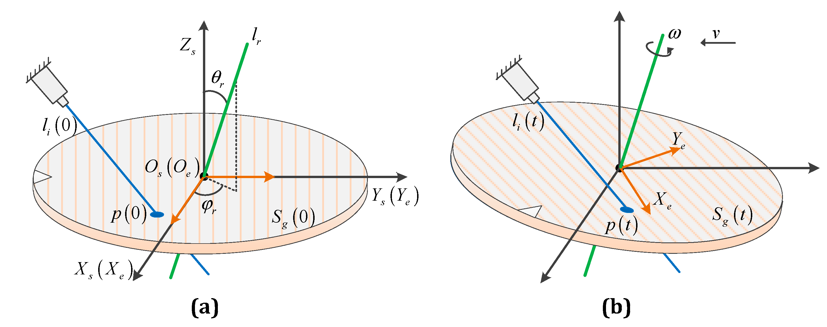
Figure 4 presents the schematic of practical system state at initial time () and scanning time . With the help of this figure, this section will parameterize the system deviations described above and finally derive the coordinate of the illuminated spot to establish a mathematical model of the practical scanning trace of the SS-SDES.
According to the definition of the system coordinate system, the rotation axis is a straight line that passes through the origin . can be described, using two parameters, by the symmetric equation of the line in space:
where and are the polar and azimuthal angles of the line as shown in Figure 4a.
The optical surface is a plane that passes through the origin . Let be the plane equation of the surface at scanning time . At the initial time (), the surface is horizontal, meaning that the normal vector of is . At any scanning time , the plane equation can be obtained by rotating counterclockwise about by an angle of as
where is the rotation matrix corresponding to a rotation by an angle of about the fixed axis , which can be computed by Rodrigues’ rotation formula [21].
Since the illuminated spot is the intersection of the illumination light and the optical surface, it is required to parameterize the illumination light by a line. Let be the equation of the illumination line at scanning time :
Four parameters are included in the equation, where and are the polar and azimuthal angles of the illumination line, and is the coordinate of the initial illuminated spot. By solving the combined equation of Equations (4) and (5), one can obtain the coordinate of in the system coordinate system, denoted as ; this is subsequently transformed into the coordinate in the surface coordinate system by
where is a matrix consisting of the first two rows of the rotation matrix .
By substituting the surface coordinate of the illuminated spot, , into Equation (2), one can finally obtain the mapping relationship from the sequence number to the image coordinate . For brevity, we use to denote the mapping relationship, and therefore, the mapping function can be written as
where is the union of all parameters involved in the modeling, called the system parameter vector, which determines the mapping relationship . In the practical implementation, the mapping function, Equation (7), is calculated by the following 7 steps:
- Step 1:
- Calculate the corresponding scanning time of the sequence number, as ;
- Step 2:
- Define the line equation of the rotation axis using Equation (3) with parameters and ;
- Step 3:
- Calculate the plane equation of the sample surface after rotation about the rotation axis using Equation (4) with the parameter ;
- Step 4:
- Define the line equation of the illumination line using Equation (5) with parameters and ;
- Step 5:
- Calculate the intersection point of the sample plane and the illumination line;
- Step 6:
- Transform the coordinate of the intersection point from the system coordinate system to the surface coordinate system using Equation (6) with parameters , and ;
- Step 7:
- Transform the surface coordinate of the intersection point to the image coordinate using Equation (2) with parameters and .
It can be found that the ideal scanning trace, introduced in Section 2.2, is a special case of the practical scanning trace with the ideal system parameter vector , where all the parameters are the setting values of the system, and the specific expression of the ideal mapping relationship is given by Equations (1) and (2). Apparently, to reconstruct an undistorted image, an accurate system parameter vector is required for establishing the actual scanning trace and mapping relationship.
3.2. System Calibration Method
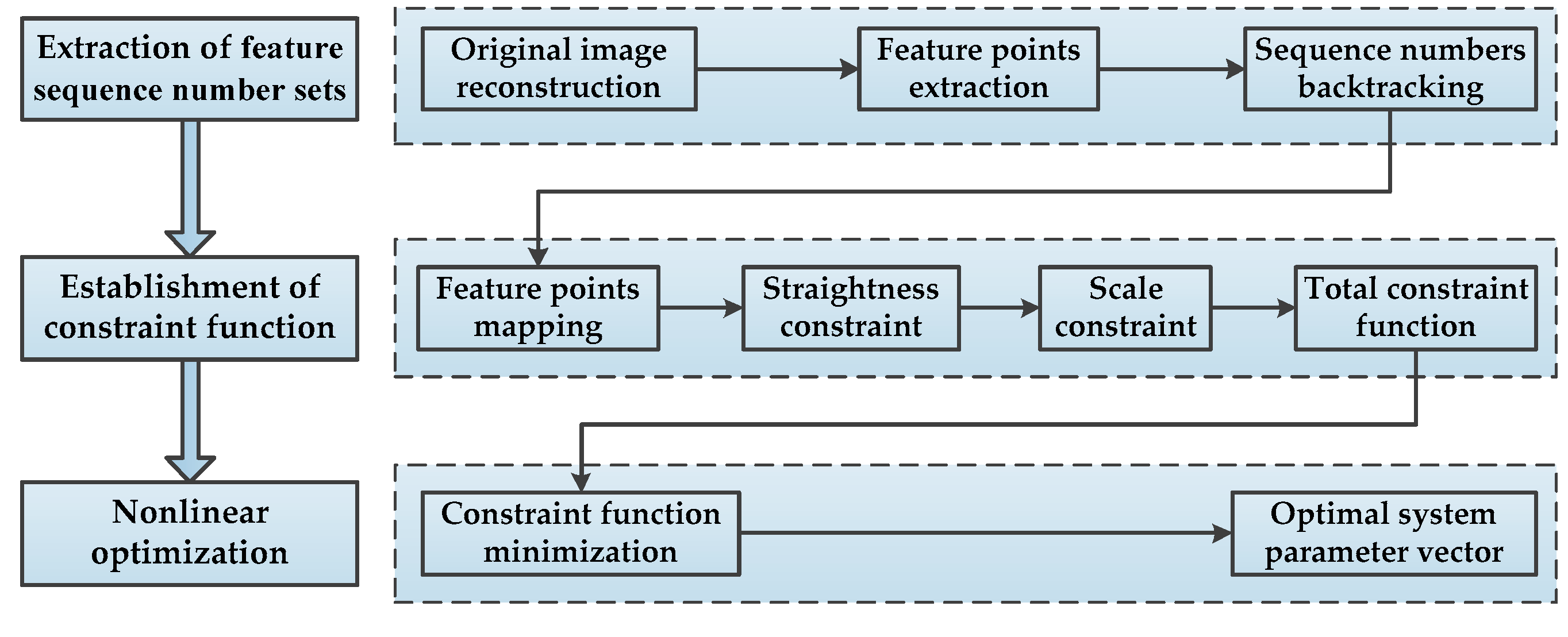
A system calibration method capable of getting the accurate system parameter vector is studied here. In this method, a specific calibration plate with a group of line-like scratches and distance-marked dot pairs on its surface is employed as the test sample. The distance-marked dot pair refers to a pair of point-like defects, such as digs, between which the distance is known. As can be found in Figure 5, this method can be divided into three major steps. The first step is to extract the feature sequence number sets, which consist of the sequence numbers of intensity signals that come from the defects. In the second step, a constraint function for constraining the image coordinates mapped from the feature sequence number sets is defined, and the third step is to perform a nonlinear optimization to minimize the constraint function, so that the optimal system parameter vector can be obtained. More details about these three steps will be given in the following.
3.2.1. Extraction of Feature Sequence Number Sets
The discrete intensity sequence acquired by the SS-SDES is one-dimensional. For each intensity signal in the sequence, although its magnitude can be used to roughly distinguish whether it is a defect signal, directly determining the location and characteristics of the defect to which the signal belongs is not possible. Hence, for the extraction of the sequence numbers corresponding to specific defects on the calibration plate, an image is first reconstructed using the ideal mapping relationship , called the original image. Then, image processing techniques are performed to find out the specific scratches and distance-marked dot pairs and to subsequently extract their feature points, which indicate the centroid for digs and the points on the skeleton for scratches. Finally, the sequence numbers corresponding to these feature points are obtained through a backtracking strategy: the discrete intensity sequence is traversed again to calculate the image coordinate for each sequence number; if the distance between the coordinate and any a feature point is less than 0.5 pixel, the sequence number is considered to correspond to this feature point. In addition, multiple groups of scratches and distance-marked dot pairs are selected to make the feature points locate at every part of the image as much as possible. Let be the number of selected scratches and be the number of selected distance-marked dot pairs. The obtained feature sequence number sets associated with them can be expressed by Equations (8) and (9), respectively:
where is the sequence number, and represents the number of sequence numbers in the th scratch, and represents the actual distance between the th distance-marked dot pairs.
3.2.2. Establishment of Constraint Function
For an arbitrary system parameter vector , the mapping relationship can be obtained according to the practical scanning trace model established in Section 3.1. By using , one can compute the image coordinates of each feature sequence number set and then observe the appearance of the corresponding defect in the reconstructed image. To avoid image distortions, our method will place two types of constraints on these coordinates. First, straight scratches should not be bent in the reconstructed image, meaning that all sequence numbers in each are expected to map to image coordinates which are collinear. Hence a straightness constraint is required. As is known, the distance of a point to a line determined by two endpoints and is , where
is the unit normal vector of the line. and denote the operations that return the absolute value of a scalar and the L2-norm of a vector, respectively. For the th selected scratch, assuming that its two endpoints correspond to the first and last sequence numbers in , the straightness constraint for can be defined by the maximum straightness error as
Second, scaling is not permitted in the reconstructed image, otherwise the relationship between the pixel size and the actual size will be changed, making the extracted geometric features of defects inaccurate. As described in Section 2.2, , the actual size of each pixel in the reconstructed image, is a fixed preset value. To maintain this characteristic, a scale constraint, for constraining the two sequence numbers in each to map to two image coordinates between which the distance is equivalent to the actual value , is constructed by the distance error , whose expression is given by
Finally, the total constraint function is defined as a weighted sum of the squares of straightness constraints and scale constraints:
where is the weight factor used to adjust the relative importance between the two types of constraints.
3.2.3. Nonlinear Optimization
Since characterizes the distortion of the reconstructed image, the optimal estimate of the system parameter vector, called the calibrated system parameter vector , can be obtained by minimizing it:
This is a nonlinear least-squares problem. As the number of variables increases, the problem becomes more complex. In the modeling of the practical scanning trace, it can be found that for the three variables, ,, and , the mapping relationship is actually related only to and . Therefore, the sampling frequency can be fixed to the setting value with only and to be optimized, thus reducing one variable. To address this issue, the Levenberg–Marquardt Algorithm [22] is employed after comparison to other optimization algorithms. It requires an initial guess of which can be set as the ideal system parameter vector .
3.3. System Adjustment and Image Reconstruction Method
Once the calibrated system parameter vector is obtained, the corresponding calibrated mapping relationship can be established to reconstruct an image free of distortions. However, because of the position deviation between the initial illuminated spot and the origin, the undetected area is still present at the central part of the surface and the image. Thus, it is required to adjust the system to make them coincide. The adjustment method is to move the two-dimensional translation stage from its original position by distances of and along the X and the Y directions, respectively, and take this position as the starting point of scanning. The values of and are dependent on the thickness of the sample to be detected. Let be the thickness difference between the sample and the calibration plate. When , the origin , which is the intersection of the rotation axis and the surface, will shift, leading to the changes of the coordinate of the initial illuminated spot. Assuming that the sample’ surface is always on the focal plane of the ellipsoidal mirror, we can derive the expression of and using simple geometric relations as
where and are the parameters that represent the coordinate of the initial illuminated spot in .
After adjustment, the SS-SDES can perform the scan for the whole optical surface in a normal way but without any missing area at the center. Let be the system parameter vector of the adjusted system. Apparently, is the same as except that the values of parameters and are equal to zero. The adjusted mapping relationship is then constructed to map the discrete intensity sequence acquired by the adjusted system to image coordinates. This is a mapping transformation from one dimension to two dimensions, and there still exist some problems to be addressed. First, the resulting coordinates are generally non-integral, failing to meet the regulation that requires the image coordinate of each pixel to be integral. Second, because the sampling frequency and the scanning velocity are fixed during scanning, the density of sampling points in the central area of the surface will be much higher than that in the edge. As a consequence, the pixel in the central part of the reconstructed image may correspond to more than one sequence number while some pixels in the edge correspond to zero. Aiming at these problems, this paper proposes an image reconstruction method based on weighted average as follows:
- Initialize an image matrix and a weight matrix with the same size determined by the actual scanning range and ; initialize the sequence number ;
- Calculate the image coordinate corresponding to the sequence number by , and round it to the integer coordinate ; define a weight value according to the distance between them as ;
- Update the image matrix by with , the corresponding intensity in the acquired discrete intensity sequence, and the weight matrix by ;
- Update the sequence number by ; if the traversal has not been completed (i.e., ), go back to step 2;
- Compute the element-wise quotient of the two matrices, i.e., ;
- Find the positions at which the elements in have the value of zero and fill the elements at these positions in (no-value pixels) using the average of 8-neighborhood.
The output is the ultimate reconstructed image. This method can not only solve the problems of non-integral coordinates and no-value pixels, but also suppress the signal noise through the weighted average strategy. For any detection system based on spot scanning, this method can effectively improve the quality of the reconstructed image.
4. Experiment Results and Discussions
4.1. Test Environment
Experiments on the proposed system calibration method and image reconstruction method were carried out and are presented in this section. The test platform is the SS-SDES introduced in Section 2.1. A 406-nm laser is used to illuminate the optical surface at a particular angle with and . The setting value of the angular velocity of the rotation stage (ND110-65FS-S204, NIKKI DENSO) is rad/s, and the translation velocity of the two-dimensional translation stage (custom made, positioning accuracy 3 µm) is µm/s. Therefore, the actual size of each pixel is µm/pixel. The sampling frequency is Hz.
A standard plate fabricated through electron beam exposure (EBE) [23] and ion beam etching (IBE) [24] was employed as the test sample. It is a 127 mm 127 mm square fused silica plate with a thickness of 2.54 mm. A group of standard defects with different sizes, such as scratches and digs, are etched on its surface. The minimum scratch width is 0.5 µm, followed by 1, 2, 3, …, 40 µm. Thus, the scratches can be used for the establishment of straightness constraints, and the dig pairs with known distances can be used for scale constraints. The system calibration and image reconstruction methods are executed on Matlab (R2011b), Windows 7 64-bit operating system (Intel Xeon E3-1535M v5 processor, 16 Gb DDR4 2133 MHz memory).
It is worth mentioning that under these setting values, it takes nearly 70 min to scan the entire standard plate. The scanning speed depends on the translation velocity . In order to keep the pixel resolution unchanged, when one increases the translation velocity, the rotation velocity must be increased accordingly. However, in our experiment, the rotation stage we used cannot provide a higher rotation velocity on the premise of stability, thus limiting the scanning efficiency. Nevertheless, this will not affect the verification of the proposed system calibration and image reconstruction methods. In the practical application of defect detections, the rotation velocity can be increased by replacing the rotation stage with a faster one, so as to improve the scanning speed.
4.2. Experiments of System Calibration
The test sample is first scanned by the SS-SDES before adjustment. According to the setting values, the ideal system parameter vector is . The corresponding mapping relationship is then established using the practical scanning trace model as described in Section 3.1. Figure 6a shows the original image reconstructed using . As can be seen, apparent distortions are present in the image, but most defects remain independent and distinguishable, allowing the original image to be used for the extraction of feature sequence number sets.
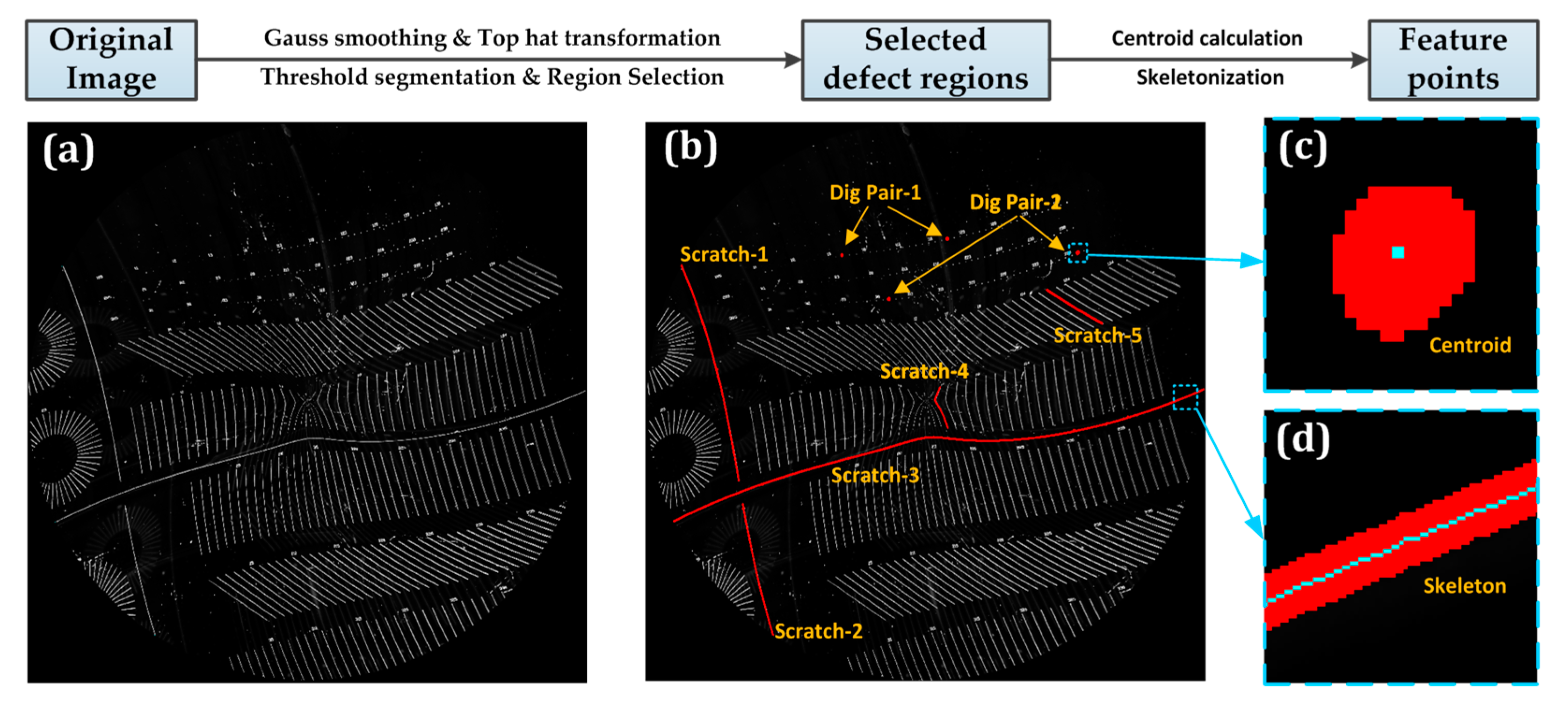
The extraction process of feature points is illustrated in Figure 6. Image processing techniques including Gauss smoothing, top hat transformation, threshold segmentation, and region selection are performed on the original image successively, to find out the regions of the specific scratches and dig pairs that are used for constraints establishment. The feature points are then extracted through skeletonization for scratches and centroid calculation for digs. Figure 6b shows some of the selected defect regions, and Figure 6c,d shows the extracted feature points of a dig and a scratch, respectively. In the calibration experiment, ten scratches and ten distance-marked dot pairs are selected. They are distributed in various parts of the image so that constraints are applied as much as possible to the entire image. With the feature points, the feature sequence number sets are obtained through the backtracking strategy, as described in Section 3.2, to subsequently construct the constraint function.
Taking as the initial guess, the Levenberg–Marquardt Algorithm is performed to obtain the calibrated system parameter vector , completing the whole process of the proposed system calibration method. The nonlinear optimization takes about 46 s, and the weight factor is chosen through experimental comparison. Table 1 gives the system calibration results where the rotation velocity is in the unit of revolutions per second (RPS). It can be seen that the calibrated values of most parameters deviate from the setting values slightly, except the azimuthal angle of rotation axis and the coordinate of the initial illuminated spot . The former is due to the fact that the rotation axis may tilt towards any azimuth in space, and the latter is caused by the lack of registration during system assembly. What is more important, shown in Table 1, is that the value of the constraint function decreases significantly after calibration, indicating that the distortion of the image is well corrected.
4.3. Experiments of Image Reconstruction
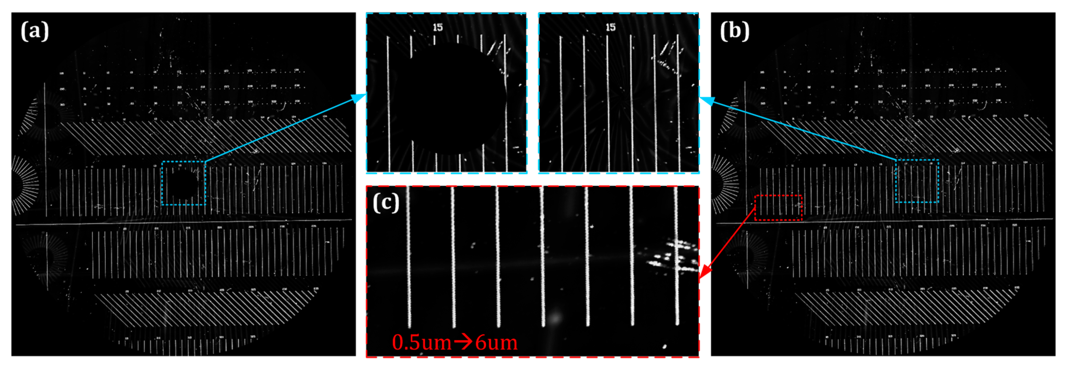
To test the validity of the system calibration method, the calibrated mapping relationship is established to reconstruct an image, called the calibrated image, for the acquired discrete intensity sequence again. Figure 7a presents the calibrated image with an enlarged image of its central area. Compared to the original image (see Figure 6a), the calibrated image shows almost no distortion but a missing area at the center, agreeing with the analysis in Section 3.3.
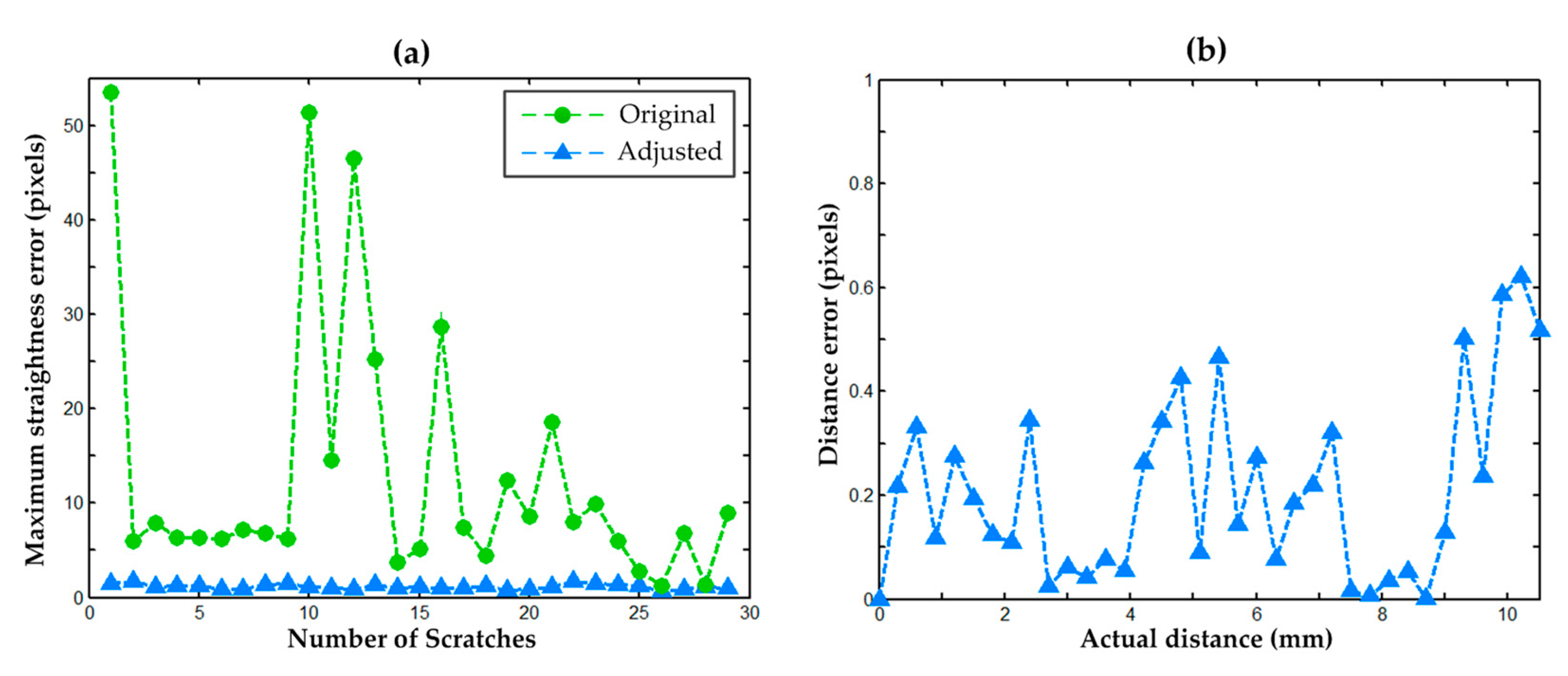
Then, the SS-SDES is adjusted as described in Section 3.3 to scan the standard plate once again and acquire the discrete intensity sequence for image reconstruction. Figure 7b presents the resulting image, called the adjusted image, which is reconstructed using the adjusted system parameter vector . It can be observed that the missing area at the center does not exist while the adjusted image remains undistorted. Moreover, Figure 7c presents an enlarged image of the scratches with widths of 0.5–6 µm. All of them can be identified clearly with high contrasts. Therefore, it can be estimated that the minimum detectable size of the SS-SDES is less than 0.5 µm. For a quantitative evaluation of the image distortion, the maximum straightness errors and the distance errors introduced above are computed for the scratches and dig pairs in the image after extraction of feature points. Figure 8a shows the maximum straightness errors comparison for different scratches between the original image (marked by circles) and the adjusted image (marked by triangles). It can be observed that some of the errors in the original image are more than 50 pixels, while those in the adjusted image are all within 1.8 pixels. The reduction is significant. Figure 8b presents the distance errors of dig pairs in the adjusted image, plotted by the actual distance on the horizontal axis. As can be seen, the distance errors are within 0.7 pixels for all the dig-pairs with different actual distances that range from 0 to about 11 mm. It means that in a defect detection based on this image, the actual geometric features of defects, such as location and length, can be extracted with subpixel accuracy. Since there is a certain error in the extraction of feature points, the results about the distortion correction are acceptable.
Additionally, to verify the effectiveness of the proposed image reconstruction method based on weighted average, the nearest-neighbor interpolation method [25] is exploited to reconstruct another image as a comparison. Figure 9 presents the gray value distributions in particular background areas of the images reconstructed by the proposed method (on the left) and the nearest-neighbor interpolation method (on the right). Figure 9a,b corresponds to a same area near the image center, with the gray value standard deviation of 0.98 and 2.48, respectively. As can be seen, the proposed method can produce a more uniform background, which is important for the following image processing to extract defects. As for the background area far from the center, as shown in Figure 9c,d, our method can eliminate the no-value pixels effectively. However, the fluctuation of background gray values, mainly caused by the signal noise, increases compared to the area near the center, with an improved gray value standard deviation of 2.16. The reason is that the density of sampling points gradually decreases from the center to the outside. Since the PMT detection duration can be shorter than 1 microsecond, if a higher sampling frequency such as MHz is employed, this problem will be mitigated, and a better noise level can be obtained. Apparently, in contrast to the nearest-neighbor interpolation method, our method has a better performance. In conclusion, the above experimental results show that with the proposed system calibration and image reconstruction methods, a complete defect image with low noise and low distortion can be obtained, thus improving the detection accuracy and reliability of the system.
5. Conclusions
A spot scanning surface defect evaluation system, which has better performances on the detection for small defects and defect classification than the traditional systems, is established. However, subject to the existing deviations, the system cannot directly provide a high-quality defect image. This paper develops research on these system deviations and then establishes the mathematical model of the practical scanning trace. On this basis, a system calibration method based on straightness and scale constraints is proposed. This method employs a calibration plate with specific defect patterns as the test sample, and places particular straightness constraints and scale constraints on the defects after being extracted. By minimizing the constraints, one can obtain the optimal estimate of the system deviations, which is used, on the one hand, to adjust the system for eliminating the position deviation of the initial illuminated spot, and on the other hand, to establish an accurate mapping relationship for reducing the distortion of the reconstructed image. The adjusted system can perform the detection for the whole optical surface in a normal way but without any missing area at the center. Additionally, an image reconstruction method based on weighted average, capable of eliminating no-value pixels and suppressing signal noise, is proposed, thus enhancing the quality of the reconstructed defect image. Finally, experiments demonstrate the effectiveness of the proposed methods, with the results that the maximum straightness error is within 1.8 pixels and the scale error is within 0.7 pixels. Our methods provide the defect image data with high quality and high precision for the following image processing to extract defects, and hence lay the foundation for improving the detection accuracy of the system. The research results of this paper can also be applied to similar problems of other detection systems based on spot scanning, such as those for wafers, films, and rough surfaces. In the future, more constraints will be considered to improve the accuracy of the system calibration method. Our system can be further improved in two ways: (1) The raw data acquired by the system contains higher-resolution information, which can be utilized to improve the detection accuracy. (2) Collecting and detecting the specular reflection light can provide additional potentials to system adjustment and defect detection.
Author Contributions
Conceptualization, Y.Y., P.C., and F.W.; methodology, F.W.; software, Y.D.; validation, F.W., P.C. and H.H.; formal analysis, F.W.; investigation, Y.D.; resources, P.C.; data curation, H.H.; writing—original draft preparation, F.W.; writing—review and editing, Y.Y.; visualization, P.C.; supervision, Y.Y.; project administration, P.C.; funding acquisition, Y.Y. All authors have read and agreed to the published version of the manuscript.
Funding
This research was supported by National Natural Science Foundation of China (NSFC, grant numbers 61627825, 61875173) and the State Key Laboratory of Modern Optical Instrumentation of Zhejiang University.
Conflicts of Interest
The authors declare no conflict of interest.
References
- Thompson, C.E.; Knopp, C.F.; Decker, D.E. Optics damage inspection for the NIF. In Proceedings of the Third International Conference on Solid State Lasers for Application to Inertial Confinement Fusion, Monterey, CA, USA, 7–12 June 1998; pp. 921–933. [Google Scholar]
- Demos, S.; Staggs, M.; Minoshima, K.; Fujimoto, J. Characterization of laser induced damage sites in optical components. Opt. Express 2002, 10, 1444–1450. [Google Scholar] [CrossRef] [PubMed]
- Kegelmeyer, L.M.; Clark, R.; Leach, R.R., Jr.; Mcguigan, D.; Kamm, V.M.; Potter, D.; Salmon, J.T.; Senecal, J.; Conder, A.; Nostrand, M. Automated optics inspection analysis for NIF. Fusion Eng. Des. 2012, 87, 2120–2124. [Google Scholar] [CrossRef]
- Pishkenari, H.N.; Meghdari, A. Surface defects characterization with frequency and force modulation atomic force microscopy using molecular dynamics simulations. Curr. Appl. Phys. 2010, 10, 583–591. [Google Scholar] [CrossRef]
- Ota, H.; Hachiya, M.; Ichiyasu, Y.; Kurenuma, T. Scanning surface inspection system with defect-review SEM and analysis system solutions. Hitachi Rev. 2006, 55, 78–82. [Google Scholar]
- Choi, W.J.; Ryu, S.Y.; Kim, J.K.; Kim, J.Y.; Kim, D.U.; Chang, K.S. Fast mapping of absorbing defects in optical materials by full-field photothermal reflectance microscopy. Opt. Lett. 2013, 38, 4907–4910. [Google Scholar] [CrossRef] [PubMed]
- Rainer, F.; Dickson, R.K.; Jennings, R.T.; Kimmons, J.F.; Maricle, S.M.; Mouser, R.P.; Schwartz, S.; Weinzapfel, C.L. Development of practical damage mapping and inspection systems. In Proceedings of the Third International Conference on Solid State Lasers for Application to Inertial Confinement Fusion, Monterey, CA, USA, 7–12 June 1998; pp. 556–563. [Google Scholar]
- Kim, G.B. A structured mechanism development and experimental parameter selection of laser scattering for the surface inspection of flat-panel glasses. Int. J. Prod. Res. 2010, 48, 3911–3923. [Google Scholar] [CrossRef]
- Tao, X.; Zhang, Z.; Zhang, F.; Xu, D. A novel and effective surface flaw inspection instrument for large-aperture optical elements. IEEE Trans. Instrum. Meas. 2015, 64, 2530–2540. [Google Scholar]
- Kim, M.S.; Choi, H.-S.; Lee, S.H.; Kim, C. A high-speed particle-detection in a large area using line-laser light scattering. Curr. Appl. Phys. 2015, 15, 930–937. [Google Scholar] [CrossRef]
- Liu, D.; Yang, Y.; Wang, L.; Zhuo, Y.; Lu, C.; Yang, L.; Li, R. Microscopic scattering imaging measurement and digital evaluation system of defects for fine optical surface. Opt. Commun. 2007, 278, 240–246. [Google Scholar] [CrossRef]
- Yongying, Y.; Chunhua, L.; Jiao, L. Microscopic dark-field scattering imaging and digitalization evaluation system of defects on optical devices precision surface. Acta Opt. Sin. 2007, 27, 1031–1038. [Google Scholar]
- Liu, D.; Wang, S.; Cao, P.; Li, L.; Cheng, Z.; Gao, X.; Yang, Y. Dark-field microscopic image stitching method for surface defects evaluation of large fine optics. Opt. Express 2013, 21, 5974–5987. [Google Scholar] [CrossRef] [PubMed]
- Li, C.; Yang, Y.; Chai, H.; Zhang, Y.; Wu, F.; Zhou, L.; Yan, K.; Bai, J.; Shen, Y.; Xu, Q. Dark-field detection method of shallow scratches on the super-smooth optical surface based on the technology of adaptive smoothing and morphological differencing. Chin. Opt. Lett. 2017, 15, 081202. [Google Scholar]
- Li, L.; Liu, D.; Cao, P.; Xie, S.; Li, Y.; Chen, Y.; Yang, Y. Automated discrimination between digs and dust particles on optical surfaces with dark-field scattering microscopy. Appl. Opt. 2014, 53, 5131–5140. [Google Scholar] [CrossRef] [PubMed]
- Takami, K. Defect inspection of wafers by laser scattering. Mater. Sci. Eng. B 1997, 44, 181–187. [Google Scholar] [CrossRef]
- Zhang, Z. A flexible new technique for camera calibration. IEEE Trans. Pattern Anal. Mach. Intell. 2000, 22, 1330–1334. [Google Scholar] [CrossRef] [Green Version]
- Wang, S.; Liu, D.; Yang, Y.; Chen, X.; Cao, P.; Li, L.; Yan, L.; Cheng, Z.; Shen, Y. Distortion correction in surface defects evaluating system of large fine optics. Opt. Commun. 2014, 312, 110–116. [Google Scholar] [CrossRef]
- Wu, F.; Du, Y.; Zhang, P.; Li, Y.; Yang, Y. Detection and discrimination of particles on and below smooth surfaces by laser scattering with polarization measurement. In Proceedings of the Applied Optical Metrology III, San Diego, CA, USA, 11–15 August 2019; p. 111021. [Google Scholar]
- Wu, F.; Yang, Y.; Jiang, J.; Zhang, P.; Li, Y.; Xiao, X.; Feng, G.; Bai, J.; Wang, K.; Xu, Q. Classification between digs and dust particles on optical surfaces with acquisition and analysis of polarization characteristics. Appl. Opt. 2019, 58, 1073–1083. [Google Scholar] [CrossRef] [PubMed]
- Brockett, R.W. Robotic manipulators and the product of exponentials formula. In Proceedings of the MTNS-83 International Symposium, Beer Sheva, Israel, 20–24 June 1983; pp. 120–129. [Google Scholar]
- Moré, J.J. The Levenberg-Marquardt algorithm: Implementation and theory. In Proceedings of the Biennial Conference, Dundee, Scotland, 28 June–1 July 1977; pp. 105–116. [Google Scholar]
- Mohammad, M.A.; Muhammad, M.; Dew, S.K.; Stepanova, M. Fundamentals of electron beam exposure and development. In Nanofabrication; Stepanova, M., Dew, S., Eds.; Springer: Vienna, Austria, 2012; pp. 11–41. [Google Scholar]
- Guzhov, V.Y. Ion-beam etching technology in the production of optical elements. J. Opt. Technol. 2002, 69, 685–687. [Google Scholar] [CrossRef]
- Bovik, A.C. Basic Gray-Level Image Processing. In Handbook of Image and Video Processing, 2nd ed.; Bovik, A.L., Ed.; Academic Press: Burlington, MA, USA, 2005; pp. 21–37. [Google Scholar]
Figure 1.
Layout of the spot scanning surface defect evaluation system.

Figure 2.
Schematic of the ideal scanning. (a) System state at scanning time ; (b) Scanning trace and the distribution of sampling points (for intuitive understanding the spacing is enlarged).
Figure 2.
Schematic of the ideal scanning. (a) System state at scanning time ; (b) Scanning trace and the distribution of sampling points (for intuitive understanding the spacing is enlarged).

Figure 3.
Simulated practical scanning traces (upper row) and the corresponding images (lower row) reconstructed using the ideal scanning trace with different system deviations. (a) Ideal case; (b) Angle deviation of the rotation axis; (c) Position deviation of the initial illuminated spot; (d) Rotation velocity deviation.

Figure 4.
Schematic of system state at different time during practical scanning. (a) Initial time (); (b) Scanning time .
Figure 4.
Schematic of system state at different time during practical scanning. (a) Initial time (); (b) Scanning time .

Figure 5.
Flow chart of the system calibration method.

Figure 6.
Flow chart of the extraction of feature points and corresponding images. (a) Original image; (b) Selected defect regions; (c) Feature point of a dig; (d) Feature points of a scratch.
Figure 6.
Flow chart of the extraction of feature points and corresponding images. (a) Original image; (b) Selected defect regions; (c) Feature point of a dig; (d) Feature points of a scratch.

Figure 7.
Reconstructed images after system calibration. (a) Calibrated image; (b) Adjusted image; (c) Enlarged image of the scratches with widths of 0.5–6 µm.
Figure 7.
Reconstructed images after system calibration. (a) Calibrated image; (b) Adjusted image; (c) Enlarged image of the scratches with widths of 0.5–6 µm.

Figure 8.
(a) The maximum straightness errors of scratches in the adjusted image with comparison to those in the original image; (b) The distance errors of dig pairs in the adjusted image.
Figure 8.
(a) The maximum straightness errors of scratches in the adjusted image with comparison to those in the original image; (b) The distance errors of dig pairs in the adjusted image.

Figure 9.
Gray value distributions in a background area near the center (upper row) and a background area far from the center (lower row) of the reconstructed images with different methods: (a,c) The proposed image reconstruction method; (b,d) The nearest-neighbor interpolation method.
Figure 9.
Gray value distributions in a background area near the center (upper row) and a background area far from the center (lower row) of the reconstructed images with different methods: (a,c) The proposed image reconstruction method; (b,d) The nearest-neighbor interpolation method.


Table 1.
System calibration results.
| Parameter | Constraint Function | ||||||||
|---|---|---|---|---|---|---|---|---|---|
| setting value | 0 | 0 | 135 | 90 | 0 | 0 | 20 | 4 | 1.7 106 |
| calibrated value | 0.038 | 102.08 | 134.99 | 88.83 | 37.45 | 960.52 | 20.034 | 4.000060 | 54.60 |
© 2020 by the authors. Licensee MDPI, Basel, Switzerland. This article is an open access article distributed under the terms and conditions of the Creative Commons Attribution (CC BY) license (http://creativecommons.org/licenses/by/4.0/).
Share and Cite
MDPI and ACS Style
Wu, F.; Cao, P.; Du, Y.; Hu, H.; Yang, Y. Calibration and Image Reconstruction in a Spot Scanning Detection System for Surface Defects. Appl. Sci. 2020, 10, 2503. https://0-doi-org.brum.beds.ac.uk/10.3390/app10072503
AMA Style
Wu F, Cao P, Du Y, Hu H, Yang Y. Calibration and Image Reconstruction in a Spot Scanning Detection System for Surface Defects. Applied Sciences. 2020; 10(7):2503. https://0-doi-org.brum.beds.ac.uk/10.3390/app10072503
Chicago/Turabian StyleWu, Fan, Pin Cao, Yubin Du, Haotian Hu, and Yongying Yang. 2020. "Calibration and Image Reconstruction in a Spot Scanning Detection System for Surface Defects" Applied Sciences 10, no. 7: 2503. https://0-doi-org.brum.beds.ac.uk/10.3390/app10072503
Note that from the first issue of 2016, this journal uses article numbers instead of page numbers. See further details here.