Synthesis of the Inverse Kinematic Model of Non-Redundant Open-Chain Robotic Systems Using Groebner Basis Theory

Featured Application

Development of a systematic procedure to synthesize the Inverse Kinematic Model of non-redundant open-chain robotic systems by the application of Groebner Basis theory.

Abstract

One of the most important elements of a robot’s control system is its Inverse Kinematic Model (IKM), which calculates the position and velocity references required by the robot’s actuators to follow a trajectory. The methods that are commonly used to synthesize the IKM of open-chain robotic systems strongly depend on the geometry of the analyzed robot. Those methods are not systematic procedures that could be applied equally in all possible cases. This project presents the development of a systematic procedure to synthesize the IKM of non-redundant open-chain robotic systems using Groebner Basis theory, which does not depend on the geometry of the robot’s structure. The inputs to the developed procedure are the robot’s Denavit–Hartenberg parameters, while the output is the IKM, ready to be used in the robot’s control system or in a simulation of its behavior. The Groebner Basis calculation is done in a two-step process, first computing a basis with Faugère’s F4 algorithm and a grevlex monomial order, and later changing the basis with the FGLM algorithm to the desired lexicographic order. This procedure’s performance was proved calculating the IKM of a PUMA manipulator and a walking hexapod robot. The errors in the computed references of both IKMs were absolutely negligible in their corresponding workspaces, and their computation times were comparable to those required by the kinematic models calculated by traditional methods. The developed procedure can be applied to all Cartesian robotic systems, SCARA robots, all the non-redundant robotic manipulators that satisfy the in-line wrist condition, and any non-redundant open-chain robot whose IKM should only solve the positioning problem, such as multi-legged walking robots.

1. Introduction

The modeling and design of a robot’s control system begins with the resolution of its kinematic problem, which is divided into two parts: the computation of the robot’s Forward Kinematics and the synthesis of the Inverse Kinematic Model (IKM).

The robot’s Forward Kinematics is the equation system that calculates the position and orientation of a specific point of the robot’s structure according to the actual state of all its actuators. This point is normally an important point of its structure, such as the end effector of a robotic arm or the center of mass of a mobile robot. The Forward Kinematics is necessary for modeling the robot’s movements, and it is also important for the synthesis of the Inverse Kinematic Model (IKM).

The IKM function is to calculate the control references required by the robot’s actuators, so the robotic system can reach a desired position or follow a predetermined path. This makes the IKM a fundamental part of the robot’s control system, as presented in Figure 1.

There are different procedures to compute the Forward Kinematics of an open-chain robotic system, which include Denavit–Hartenberg’s algorithm [1,2,3], dual quaternions [4,5], and the modeling by Displacement Matrices [6]. All these procedures calculate the Forward Kinematics through the execution of systematic algorithms, which are completely independent of the mechanical complexity of the robot’s structure or its geometry.

On the other hand, the Inverse Kinematic Problem of open-chain robotic systems presents a greater challenge because the most commonly used methods to calculate the IKM, the geometric method, and the analytical method strongly depend on the analyzed robot’s geometry and do not offer a systematic procedure for the synthesis of the desired model. The geometric method divides the analyzed robot Inverse Kinematic Problem into several plane geometry problems, and solves those problems using trigonometric relations [3,7]. It is obvious, by its own definition, that this method depends heavily on the geometry of the robot’s structure, and any sequence of steps used to calculate the IKM of a robotic system may not be valid for any other different structure.

The analytic method for the calculation of the IKM solves the state vector of the robot’s actuators in the equation system that defines the Forward Kinematics [8,9,10]. The drawback of this method is that the aforementioned equation system is composed of nonlinear equations, which forbids the use of traditional matrix algebra procedures. Instead, individual relations inside the analyzed equation system must be found, relations that are specific for each case. This implies that the analytic method is also non-systematic because the relations found to calculate the IKM of a robot with a certain structure, may not be valid or suitable for a different robot.

All the problems presented before have prompted the development of several projects that use different artificial intelligence techniques to solve the Inverse Kinematic Problem, such as Neural Networks [11,12,13], Particle Swarm Optimization (PSO) [14], PSO-optimized Neural Networks [15], Neuro-evolutionary Algorithms (combination of Neural Networks and Genetic Algorithms) [16], and PSO variants [17]. These techniques normally calculate satisfactory solutions for the Inverse Kinematic Problem (IKP), without having any problems with the geometry of the robot’s structure. However, it is important to clarify that, while these methods solve the IKP, they do not synthesize an Inverse Kinematic Model (IKM). This implies that the position references that are offered as output do not come from a differentiable function; therefore, these procedures are not capable of computing the speed or acceleration references for the robot’s actuators. In addition, these methods could suffer from the known training problems of artificial intelligence techniques, such as the over-fitting of Neural Networks and Genetic Algorithms.

Nowadays, several projects are being developed in the field of Robotics that use Groebner Basis theory [18] to implement systematic methods that solve the Kinematic Problem, in a way that is independent of the geometry of the robot’s structure. Among these projects, the works of Kendricks [19] and Wang et al. [20] stand out, which solve the Inverse Kinematic Problem of robotic manipulators using Groebner Bases. Abbasnejad et al. [21] use this theory for the kinematic analysis of cable-driven robots. Rameau et al. [22] employ it to calculate the mobility conditions of several mechanisms that can be used in robotic arms or parallel robots. The works of Gan et al. [23] and Huang et al. [24] use Groebner Basis theory for the resolution of the Kinematic Problem of parallel robots, while Uchida et al. [25] employ it to triangularize the kinematic constraint equations of closed-chain robotic systems.

Most of the aforementioned works employ Groebner Bases to solve their corresponding Kinematic Problems, proving that the full set of solutions can be obtained using this theory. However, they do not provide a procedure to synthesize a Kinematic Model that can be used in the control system of the robot (see Figure 1).

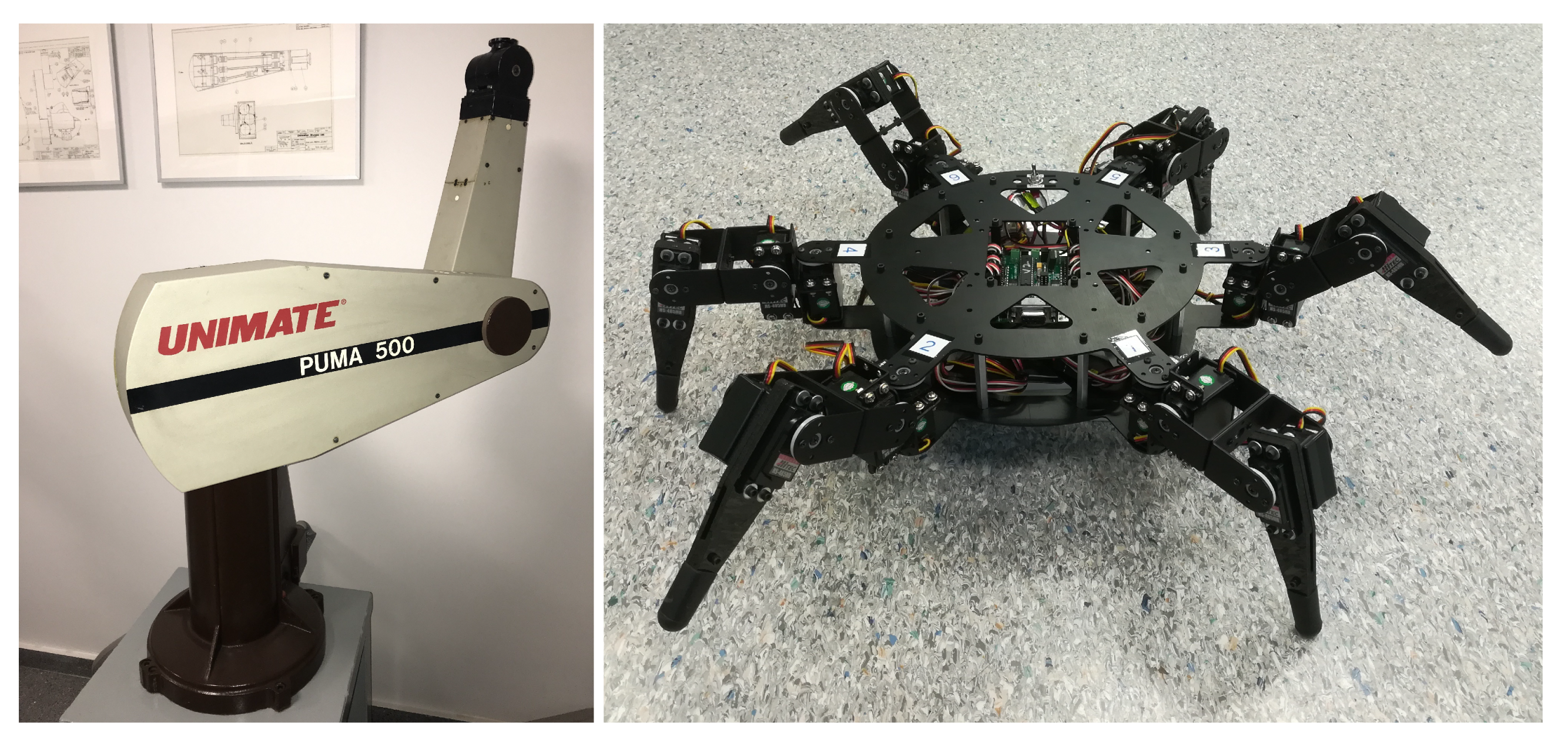
This work objective is to use Groebner Basis theory to develop a systematic procedure for the synthesis of the IKM of non-redundant open-chain robotic systems. This procedure is explained in Section 3 and was used to synthesize the IKMs of two robots: a PUMA manipulator and a walking hexapod. Section 2 presents the calculation by traditional methods of the kinematic models of the two mentioned robots, which are later used as reference models in the performance analysis of the developed procedure. Section 4 shows the procedure’s performance analysis, comparing the outputs of the IKMs synthesized in this project with those of the reference models. The possible future works that arise from this project are summarized in Section 5. In addition, finally Section 6 presents the conclusions of the obtained results and the final remarks of this work.

2. Resolution of the Kinematic Problem by Traditional Methods

The two robotic systems that were studied in this project are a Unimate’s PUMA 560 robotic arm (Danbury, CT, USA) and the walking hexapod robot BH3-R, built and distributed by Lynxmotion Inc. (Swanton, Vermont, USA). Both robots, shown in Figure 2, are non-redundant open-chain robotic systems, and they will be used as test benches for the procedure developed in this work.

The first step for the resolution of the Kinematic Problem by any of the traditional methods is to calculate the Forward Kinematics of the analyzed robot.

2.1. Forward Kinematics

The Forward Kinematics of any robotic system can be easily solved by applying the Denavit–Hartenberg’s method (D–H). The first step of this method is to establish the proper coordinate systems, following the D–H convention, as explained in [1,3].

2.1.1. Forward Kinematics of the PUMA

Figure 3 shows the coordinate systems created for all the links of the PUMA 560 robotic arm. Based on the coordinate systems presented in this figure, the D–H parameters of every link of the robot are the ones contained in

Table 1. Denavit–Hatenberg Parameters of PUMA 560.

Link	$\mathit{\theta }$	d	a	$\mathit{\alpha }$
1	$q_1+(\pi /2)$	$d_1$	0	$-\pi /2$
2	$q_2$	$d_2$	$a_2$	0
3	$q_3+(\pi /2)$	0	$-a_3$	$\pi /2$
4	$q_4$	$d_4$	0	$-\pi /2$
5	$q_5$	0	0	$\pi /2$
6	$q_6$	$d_6$	0	0

.

Table 2. Parameter dimensions of PUMA 560.

Parameter	Dimension [mm]
$d_1$	660.4
$d_2$	149.1
$a_2$	431.8
$a_3$	20.3
$d_4$	433.1
$d_6$	56.2

lists the dimensions, in mm, of these PUMA’s parameters.

For simplicity reasons, we will focus only on the first three links of the robotic arm, just before the robot’s wrist. This simplification is valid because the last three links of the arm comply with the conditions of Pieper’s Theorem [3,8], effectively conforming an in-line wrist. Therefore, the end effector of this robot will be considered to be at the anchor point of this in-line wrist, just at coordinate system number 4, shown in Figure 3.

Applying the Denavit–Hartenberg’s method, with the parameters presented in Table 1, the solution to the Forward Kinematics problem of the PUMA 560 is the homogeneous transformation shown in Equation (1), which establishes the transformation between the base of the robot and the anchor point of its in-line wrist. The term “$q_{(2+3)}$” in Equation (1) is equal to “$q_2+q_3$”.

$${}^0{A}_4=\left[\begin{array}{cccc}sin\left(q_1\right)sin\left(q_{(2+3)}\right)& sin\left(q_1\right)cos\left(q_{(2+3)}\right)& -cos\left(q_1\right)& -sin\left(q_1\right)[a_{2}cos\left(q_2\right)+d_{4}cos\left(q_{(2+3)}\right)+a_{3}sin\left(q_{(2+3)}\right)]-d_{2}cos\left(q_1\right)\\ -cos\left(q_1\right)sin\left(q_{(2+3)}\right)& -cos\left(q_1\right)cos\left(q_{(2+3)}\right)& -sin\left(q_1\right)& cos\left(q_1\right)[a_{2}cos\left(q_2\right)+d_{4}cos\left(q_{(2+3)}\right)+a_{3}sin\left(q_{(2+3)}\right)]-d_{2}sin\left(q_1\right)\\ -cos\left(q_{(2+3)}\right)& sin\left(q_{(2+3)}\right)& 0& d_1-a_{2}sin\left(q_2\right)-d_{4}sin\left(q_{(2+3)}\right)+a_{3}cos\left(q_{(2+3)}\right)\\ 0& 0& 0& 1\end{array}\right]$$

(1)

2.1.2. Forward Kinematics of the BH3-R Hexapod

The second robotic system used as a testbench in this project is the hexapod shown in Figure 2. Because this hexapod has circular geometry, its kinematic problem can be synthesized in calculating the IKM of one of the robot’s legs, to apply later the corresponding transformations between the hexapod’s center and the origin of each of its extremities. This robot was selected as a testbench because each of its legs has three rotational degrees of freedom for positioning, like most industrial robotic arms and many multi-legged walking robots, and it only requires the resolution of the positioning kinematic problem.

The calculated D–H parameters that define this robotic system are shown in

Table 3. Denavit–Hatenberg Parameters of the hexapod’s leg.

Link	$\mathit{\theta }$	d	a	$\mathit{\alpha }$
1	$q_1$	0	$L_1$	$\pi /2$
2	$q_2$	0	$L_2$	$\pi$
3	$q_3+(\pi /2)$	0	$L_3$	0

, while

Table 4. Parameter dimensions of the hexapod’s leg.

Parameter	Dimension [mm]
$L_1$	28.0
$L_2$	58.0
$L_3$	110.0

lists the dimensions, in mm, of those parameters. Finally, Equation (2) presents the homogeneous transformation between the origin of the hexapod’s leg and its final point, which was calculated following all the steps of Denavit–Hatenberg’s method [1].

$${}^0{A}_3=\left[\begin{array}{cccc}cos\left(q_1\right)sin(q_2-q_3)& -cos\left(q_1\right)cos(q_2-q_3)& -sin\left(q_1\right)& cos\left(q_1\right)[L_1+L_{2}cos\left(q_2\right)+L_{3}sin(q_2-q_3)]\\ sin\left(q_1\right)sin(q_2-q_3)& -sin\left(q_1\right)cos(q_2-q_3)& cos\left(q_1\right)& sin\left(q_1\right)[L_1+L_{2}cos\left(q_2\right)+L_{3}sin(q_2-q_3)]\\ -cos(q_2-q_3)& -sin(q_2-q_3)& 0& L_{2}sin\left(q_2\right)-L_{3}cos(q_2-q_3)\\ 0& 0& 0& 1\end{array}\right]$$

(2)

2.2. Inverse Kinematics Using Traditional Methods

2.2.1. Inverse Kinematics of the PUMA 560 by the Geometric Method

Based on the link coordinate systems presented in Figure 3, and inspired in the geometry of a human arm, various arm configurations can be identified for a PUMA robot with the assistance of three configuration indicators: ARM, ELBOW, and WRIST [3]. The first two, ARM and ELBOW, are associated with the solution of the first three joints, while WRIST is related to the solution of the last three. For a six-axis manipulator, like the PUMA 560, there are four possible solutions for the first three joints ($q_1$, $q_2$ and $q_3$), commonly referred as configurations, and for each one of these configurations, there are two possible solutions for the last three joints ($q_4$, $q_5$ and $q_6$) [3].

As was stated in Section 2.1.1, we will focus exclusively in the first three joints of the PUMA robotic arm. Thus, we only need to find the four possible solutions for $q_1$ to $q_3$, which are related to the first two configuration indicators: ARM and ELBOW.

The ARM indicator can have two possible values, LEFT and RIGHT. LEFT indicates that positive values of $q_2$ will move the robot’s wrist in the negative ${\mathbf{Z}}_{\mathbf{0}}$ direction when the third joint, $q_3$, is not activated, while RIGHT will move it in the positive ${\mathbf{Z}}_{\mathbf{0}}$ direction. ELBOW also has two possible values, ABOVE and BELOW, which indicate whether the third joint of the robot is above the imaginary line described between the top part of the robot’s body and its wrist, or below this line, respectively. The combination of the two possible values of the ARM indicator with the two of ELBOW gives the four possible configurations that constitute the four solutions of the Inverse Kinematics Problem of the PUMA 560.

If the position vector $\overrightarrow{\mathbf{p}}({\mathbf{p}}_{\mathbf{x}},{\mathbf{p}}_{\mathbf{y}},{\mathbf{p}}_{\mathbf{z}})$ is projected onto the ${\mathbf{X}}_{\mathbf{0}}-{\mathbf{Y}}_{\mathbf{0}}$ plane, as shown in Figure 4, $q_1$ could be obtained solving the equations shown in Equation (3). The “L” and “R” superscripts added to $q_1$ differentiate between the LEFT and RIGHT arm configurations.

$$\begin{array}{c}\overrightarrow{OA}=d_2\\ \overrightarrow{OE}=R_2=\sqrt{{\left(p_x\right)}^2+{\left(p_y\right)}^2}\\ \overrightarrow{AE}=r_{a2}=\sqrt{{\left(p_x\right)}^2+{\left(p_y\right)}^2-{\left(d_2\right)}^2}\\ \alpha =atan2\left({\displaystyle \frac{d_2}{R_2}},{\displaystyle \frac{r_{a2}}{R_2}}\right)\\ \phi =atan2\left({\displaystyle \frac{p_y}{R_2}},{\displaystyle \frac{p_x}{R_2}}\right)\\ q_1^L=\phi -\alpha ;q_1^R=\phi +\alpha +\pi ;\end{array}$$

(3)

To calculate $q_3$, the position vector $\overrightarrow{\mathbf{p}}$ is projected onto the plane ${\mathbf{X}}_{\mathbf{2}}-{\mathbf{Y}}_{\mathbf{2}}$, as shown in Figure 5, obtaining the geometric equations presented in Equation (4):

$$\begin{array}{c}\overrightarrow{AB}=a_2;\overrightarrow{BC}=a_3;\overrightarrow{CD}=d_4;\\ \overrightarrow{BD}=r_3=\sqrt{{\left(a_3\right)}^2+{\left(d_4\right)}^2}\\ \overrightarrow{AD}=r_{a3}=\sqrt{{\left(p_x\right)}^2+{\left(p_y\right)}^2+{\left(p_z\right)}^2-{\left(d_2\right)}^2}\\ \beta =atan2\left({\displaystyle \frac{\left|d_4\right|}{r_3}},{\displaystyle \frac{\left|a_3\right|}{r_3}}\right)\\ cos\left(\phi \right)={\displaystyle \frac{a_2^2+r_3^2-r_{a3}^2}{2·a_2·r_3}}\\ sin\left({\phi }^{LA}\right)=-\sqrt{1-cos{\left(\phi \right)}^2};sin\left({\phi }^{RA}\right)=+\sqrt{1-cos{\left(\phi \right)}^2};\\ sin\left({\phi }^{LB}\right)=+\sqrt{1-cos{\left(\phi \right)}^2};sin\left({\phi }^{RB}\right)=-\sqrt{1-cos{\left(\phi \right)}^2};\\ {\phi }^k=atan2\left(sin\left({\phi }^k\right),cos\left(\phi \right)\right)\end{array}$$

(4)

The superscript k in Equation (4) may have the values $LA$, $RA$, $LB$ or $RB$, depending on the value of the ARM and ELBOW indicators. Thus, the four possible solutions for $q_3$ can be compacted in the expression presented in Equation (5):

$$\begin{array}{c}{q}_3^k={\phi }^k-\beta \end{array}$$

(5)

Projecting the position vector $\overrightarrow{\mathbf{p}}$ onto the plane ${\mathbf{X}}_{\mathbf{1}}-{\mathbf{Y}}_{\mathbf{1}}$, as shown in Figure 6, $q_2$ is calculated solving the geometric equations presented in Equation (6).

$$\begin{array}{c}\overrightarrow{EF}=p_x;\overrightarrow{EG}=p_y;\overrightarrow{DE}=p_z;\\ \overrightarrow{AE}=r_{a2};\overrightarrow{AD}=r_{a3};\\ sin\left(\alpha \right)=-{\displaystyle \frac{p_z}{r_{a3}}}\\ cos\left({\alpha }^L\right)={\displaystyle \frac{r_{a2}}{r_{a3}}}\\ cos\left({\alpha }^R\right)=-cos\left({\alpha }^L\right)=-{\displaystyle \frac{r_{a2}}{r_{a3}}}\\ {\alpha }^i=atan2\left(sin\left(\alpha \right),cos\left({\alpha }^i\right)\right)\\ cos\left(\beta \right)={\displaystyle \frac{a_2^2+r_{a3}^2-\left(d_4^2+a_3^2\right)}{2·a_2·r_{a3}}}\\ sin\left(\beta \right)=\sqrt{1-cos\left({\beta }^2\right)}\\ \beta =atan2(sin(\beta ),cos(\beta \left)\right)\end{array}$$

(6)

In Equation (6), the superscript i could either be L or R, depending on the value of the ARM indicator. Therefore, the four possible solutions for $q_2$ are presented in Equation (7):

$$\begin{array}{c}{q}_2^{LA}={\alpha }^L-\beta ;q_2^{RA}={\alpha }^R+\beta ;\\ q_2^{LB}={\alpha }^L+\beta ;q_2^{RB}={\alpha }^R-\beta ;\end{array}$$

(7)

Finally, Equation (8) presents the four configurations structure that conforms the whole solution of the Inverse Kinematic Problem of the PUMA 560 manipulator:

$$\begin{array}{c}{q}^{LA}=\left[\begin{array}{c}{q}_1^L\\ q_2^{LA}\\ q_3^{LA}\end{array}\right]q^{RA}=\left[\begin{array}{c}{q}_1^R\\ q_2^{RA}\\ q_3^{RA}\end{array}\right]\\ q^{LB}=\left[\begin{array}{c}{q}_1^L\\ q_2^{LB}\\ q_3^{LB}\end{array}\right]q^{RB}=\left[\begin{array}{c}{q}_1^R\\ q_2^{RB}\\ q_3^{RB}\end{array}\right]\end{array}$$

(8)

2.2.2. Inverse Kinematics of the BH3-R Hexapod’s Leg by the Analytical Method

The analytical method begins with the Forward Kinematics equation system, presented in Equation (9), that calculates the position vector of the end point, $\overrightarrow{\mathbf{p}}$, from the configuration of all actuators of the hexapod’s leg ($q_1$, $q_2$ and $q_3$). In this equation, $p_{x_0}$ represents the projection of the vector $\overrightarrow{\mathbf{p}}$ over the ${\mathbf{X}}_{\mathbf{0}}$ axis, $p_{y_0}$ is the projection over ${\mathbf{Y}}_{\mathbf{0}}$, while $p_{z_0}$ constitutes the projection over ${\mathbf{Z}}_{\mathbf{0}}$:

$$\begin{array}{c}\left[\begin{array}{c}{p}_{x_0}\\ p_{y_0}\\ p_{z_0}\\ 1\end{array}\right]={}^0{A}_3·\left[\begin{array}{c}0\\ 0\\ 0\\ 1\end{array}\right]=\left[\begin{array}{c}cos\left(q_1\right)\left[L_1+L_{2}cos\left(q_2\right)+L_{3}sin(q_2-q_3)\right]\\ sin\left(q_1\right)\left[L_1+L_{2}cos\left(q_2\right)+L_{3}sin(q_2-q_3)\right]\\ L_{2}sin\left(q_2\right)-L_{3}cos(q_2-q_3)\\ 1\end{array}\right]\end{array}$$

(9)

The solution for the first actuator of the robot, $q_1$, can be obtained by dividing the second equation of the system shown in Equation (9) by the first one, as presented in Equation (10):

$$\begin{array}{c}{\displaystyle \frac{p_{y_0}}{p_{x_0}}}={\displaystyle \frac{sin\left(q_1\right)\left[L_1+L_{2}cos\left(q_2\right)+L_{3}sin(q_2-q_3)\right]}{cos\left(q_1\right)\left[L_1+L_{2}cos\left(q_2\right)+L_{3}sin(q_2-q_3)\right]}}={\displaystyle \frac{sin\left(q_1\right)}{cos\left(q_1\right)}}\Rightarrow q_1^F=arctan\left({\displaystyle \frac{p_{y_0}}{p_{x_0}}}\right)\end{array}$$

(10)

The right hand of Equation (10) shows one of the possible solutions for $q_1$, the one normally labelled as “FRONT” (F) for this type of mechanical structure. The second possible solution is the one presented in Equation (11), which also solves Equation (10). This second solution is usually identified as “BACK” (B):

$$\begin{array}{c}{\displaystyle \frac{sin\left(q_1\right)}{cos\left(q_1\right)}}={\displaystyle \frac{p_{y_0}}{p_{x_0}}}={\displaystyle \frac{-p_{y_0}}{-p_{x_0}}}\Rightarrow q_1^B=arctan\left({\displaystyle \frac{-p_{y_0}}{-p_{x_0}}}\right)=q_1^F+\pi \end{array}$$

(11)

The two possible solutions for $q_1$ are presented in Equation (12), where the arctan function has been substituted by the more general atan2, which is fully defined for all the range $[-\pi ,\pi ]$:

$$\begin{array}{c}{q}_1^F=atan2\left(p_{y_0},p_{x_0}\right);q_1^B=q_1^F+\pi ;\end{array}$$

(12)

To obtain the solution for $q_3$, we have to return to the definition of the Forward Kinematics equation system (see Equation (9)), and do the matrix operations shown in Equation (13):

$$\begin{array}{cc}\hfill \left[\begin{array}{c}{p}_{x_0}\\ p_{y_0}\\ p_{z_0}\\ 1\end{array}\right]& ={}^0{A}_3·\left[\begin{array}{c}0\\ 0\\ 0\\ 1\end{array}\right]={}^0{A}_1\left(q_1^i\right)·{}^1{A}_2·{}^2{A}_3·\left[\begin{array}{c}0\\ 0\\ 0\\ 1\end{array}\right]\hfill \\ \hfill & \Downarrow \hfill \\ \hfill {\left({}^0{A}_1\left(q_1^i\right)\right)}^{-1}·\left[\begin{array}{c}{p}_{x_0}\\ p_{y_0}\\ p_{z_0}\\ 1\end{array}\right]& ={\left({}^0{A}_1\left(q_1^i\right)\right)}^{-1}·{}^0{A}_1\left(q_1^i\right)·{}^1{A}_2·{}^2{A}_3·\left[\begin{array}{c}0\\ 0\\ 0\\ 1\end{array}\right]={}^1{A}_3·\left[\begin{array}{c}0\\ 0\\ 0\\ 1\end{array}\right]\hfill \\ \hfill & \Downarrow \hfill \\ \hfill \left[\begin{array}{c}{p}_{x_1^i}\\ p_{y_1^i}\\ p_{z_1^i}\\ 1\end{array}\right]& =\left[\begin{array}{c}{L}_{2}cos\left(q_2\right)+L_{3}sin(q_2-q_3)\\ L_{2}sin\left(q_2\right)-L_{3}cos(q_2-q_3)\\ 0\\ 1\end{array}\right]\hfill \end{array}$$

(13)

The superscript i that appears in some terms of Equation (13) may be either F (“FRONT”) or B (“BACK”), depending on the related configuration of $q_1$. The terms $p_{x_1^i}$, $p_{y_1^i}$, and $p_{z_1^i}$ represent the projection of the position vector over the ${\mathbf{X}}_{\mathbf{1}}$, ${\mathbf{Y}}_{\mathbf{1}}$, and ${\mathbf{Z}}_{\mathbf{1}}$ axes, respectively, taking into account that these axes depend on the aforementioned configuration of $q_1$.

From Equation (13), we can add the square of the first two equations of that equation system, obtaining the solution shown in Equation (14):

$$\begin{array}{c}{\left(p_{x_1^i}\right)}^2+{\left(p_{y_1^i}\right)}^2={\left[L_{2}cos\left(q_2\right)+L_{3}sin(q_2-q_3)\right]}^2+{\left[L_{2}sin\left(q_2\right)-L_{3}cos(q_2-q_3)\right]}^2\\ \Downarrow \\ {\left(p_{x_1^i}\right)}^2+{\left(p_{y_1^i}\right)}^2={\left(L_2\right)}^2+{\left(L_3\right)}^2-2L_2{L}_{3}sin\left(q_3\right)\\ \Downarrow \\ sin\left(q_3^i\right)={\displaystyle \frac{{\left(L_2\right)}^2+{\left(L_3\right)}^2-{\left(p_{x_1^i}\right)}^2-{\left(p_{y_1^i}\right)}^2}{2L_2{L}_3}}\end{array}$$

(14)

The term $sin\left(q_3^i\right)$ in Equation (14) can have two possible solutions, depending on whether the configuration of $q_1$ is F or B. Each of these solutions for $sin\left(q_3^i\right)$ yield two possible values for $cos\left(q_3\right)$ when the quadratic equation shown in Equation (15) is solved:

$$\begin{array}{c}cos\left(q_3^k\right)=\pm \sqrt{1-{\left[sin\left(q_3^i\right)\right]}^2}\end{array}$$

(15)

The four possible values for $cos\left(q_3^k\right)$ in Equation (15) lead to the expression of $q_3$ in Equation (16), where the superscript k may be $FA$ (“FRONT ABOVE”), $FB$ (“FRONT BELOW”), $BA$ (“BACK ABOVE”) or $BB$ (“BACK BELOW"). The names of these configuration identifiers were selected in a similar way as the ones of the the PUMA 560 (see Section 2.2.1):

$$\begin{array}{c}{q}_3^k=atan2\left(sin\left(q_3^i\right),cos\left(q_3^k\right)\right)\end{array}$$

(16)

Once $q_3$ has been calculated, $q_2$ may be obtained solving the equation system shown in the final part of Equation (13), as it is presented in Equation (17):

$$\begin{array}{c}sin\left(q_2^k\right)={\displaystyle \frac{p_{y_1^i}[L_2-L_{3}sin\left(q_3^i\right)]+p_{x_1^i}{L}_{3}cos\left(q_3^k\right)}{{[L_2-L_{3}sin\left(q_3^i\right)]}^2+{[L_{3}cos\left(q_3^k\right)]}^2}}\\ cos\left(q_2^k\right)={\displaystyle \frac{p_{x_1^i}-L_{3}cos\left(q_3^k\right)sin\left(q_2^k\right)}{L_2-L_{3}sin\left(q_3^i\right)}}\end{array}$$

(17)

Finally, Equation (18) presents the four configurations structure that conform the solution of the Inverse Kinematic Problem of the analyzed walking hexapod:

$$\begin{array}{c}{q}^{FA}=\left[\begin{array}{c}{q}_1^F\\ q_2^{FA}\\ q_3^{FA}\end{array}\right]q^{BA}=\left[\begin{array}{c}{q}_1^B\\ q_2^{BA}\\ q_3^{BA}\end{array}\right]\\ q^{FB}=\left[\begin{array}{c}{q}_1^F\\ q_2^{FB}\\ q_3^{FB}\end{array}\right]q^{BB}=\left[\begin{array}{c}{q}_1^B\\ q_2^{BB}\\ q_3^{BB}\end{array}\right]\end{array}$$

(18)

After analyzing the two traditional methods that are normally used to solve the Inverse Kinematics Problem, it is obvious that they are not systematic procedures because the geometric calculations done for the PUMA 560 manipulator cannot be applied to the BH3-R walking hexapod, and vice versa. Section 3 presents the procedure developed in this work to synthesize the IKM in a systematic way, using Groebner Basis theory.

3. Procedure to Synthesize the IKM Using Groebner Basis

The developed procedure for the calculation of the IKM of non-redundant open-chain robotic systems is divided into six steps:

• Information input
• Forward kinematics
• Obtention of the of the polynomial equation system
• Monomial Order selection
• Groebner Basis calculation
• Final IKM algorithm

It is important to highlight that all these steps are only executed once, out of line, to synthesize the IKM before the robotic system is activated. Therefore, the execution time of these steps does not affect in any way the online computation time of the IKM.

3.1. First Step: Information Input

The procedure begins requesting all the relevant information about the analyzed robot. The user has to supply only two data: the Denavit–Hartenberg (D–H) parameters of the robot and the movement range of its actuators.

The first data, the D–H parameters, are necessary to solve the Forward Kinematics problem, which is a required step to calculate the Groebner Basis that will constitute the IKM. These parameters represent the fundamental information of any robotic system, so they are also indispensable for all traditional methods that solve the Kinematic Problem.

The robot actuators’ movement range is employed to eliminate all the solutions that are not reachable by the robotic system. This way, the IKM is able to discard those solutions that are out of the robot’s workspace.

3.2. Second Step: Forward Kinematics

The second step in the developed procedure is the robot’s Forward Kinematics calculation, using the D–H parameters that were provided in the first step. This calculation is done applying the Denavit–Hartenberg method [1], so this part of the procedure is similar to the presented in Section 2.1 for the traditional methods.

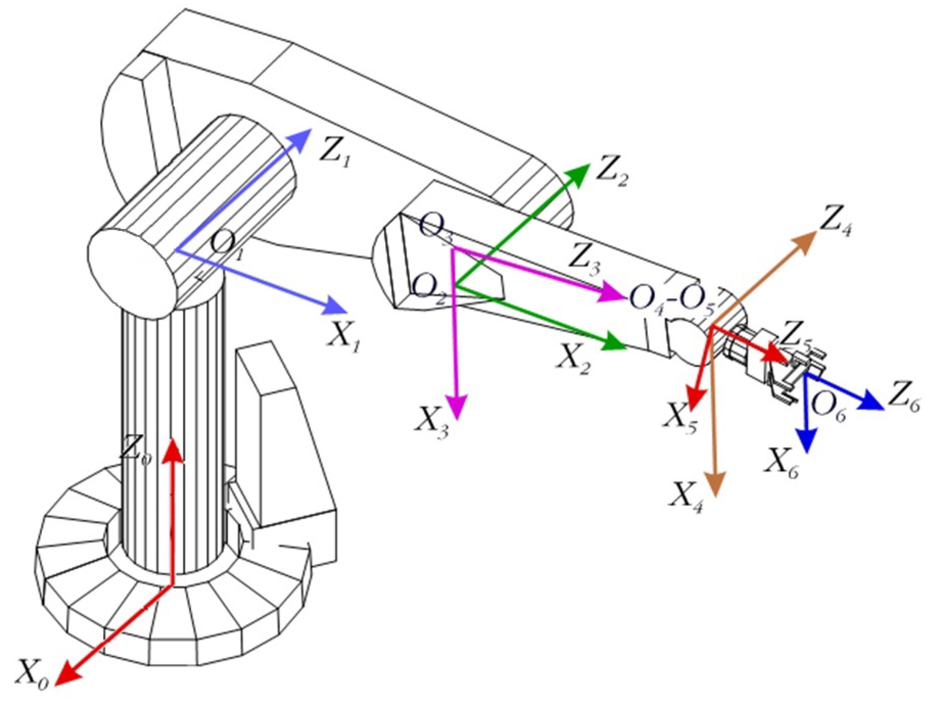
The result of this second step is the homogeneous transformation matrix (${}^0{A}_n$) between the origin of the coordinate system in the robot’s base and the one in its end effector. Therefore, after applying the developed procedure to the PUMA robot presented in Figure 3, the result of this step is the same homogeneous matrix presented in Equation (1).

3.3. Third Step: Obtention of the Polynomial Equation System

Once the robot’s Forward Kinematics is calculated, the equations that relate the pose of the end effector with the robot’s state can be extracted from the homogeneous transformation matrix obtained in the second step. In this work, for simplicity, we are only interested in the position of the end effector, which is only a part of its pose. However, all the calculations made in the developed procedure can be also extended to the orientation, to complete the whole pose.

Continuing with the case of the PUMA robot, these equations are the ones presented in Equation (19), which correspond to the first three elements of the fourth column of Equation (1):

$$\begin{array}{c}{p}_x=-sin\left(q_1\right)[a_{2}cos\left(q_2\right)+d_{4}cos(q_2+q_3)+a_{3}sin(q_2+q_3)]-d_{2}cos\left(q_1\right)\\ p_y=cos\left(q_1\right)[a_{2}cos\left(q_2\right)+d_{4}cos(q_2+q_3)+a_{3}sin(q_2+q_3)]-d_{2}sin\left(q_1\right)\\ p_z=d_1-a_{2}sin\left(q_2\right)-d_{4}sin(q_2+q_3)+a_{3}cos(q_2+q_3)\end{array}$$

(19)

As it can be seen in Equation (19), the final result obtained from the robot’s Forward Kinematics is a trigonometric equation system that establish the position of the end effector, and it is from this equation system that the calculation of the IKM begins.

The previous equation system is completed with the corresponding trigonometric identities of all the robot’s rotational degrees of freedom (DoFs), identities of the form $sin{\left(q_i\right)}^2+cos{\left(q_i\right)}^2=1$. Then, all the trigonometric expressions are expanded, and variable substitutions of the form $sin\left(q_i\right)=s_i$ and $cos\left(q_i\right)=c_i$ are applied. This step’s objective is to obtain a polynomial equation system where the variables are either a pair sine-cosine of a rotational DoF ($s_i$ and $c_i$), or directly the position value of a prismatic DoF ($q_j$).

For the case of the PUMA robot, this step’s output is the trigonometric equation system presented in Equation (20). In this equation system, $p_x$, $p_y$, and $p_z$ are the three components of the position vector of the PUMA’s wrist ($\overrightarrow{\mathbf{p}}$), and they are input parameters. The six variables of Equation (20) that should be solved are $s_1$, $c_1$, $s_2$, $c_2$, $s_3$, and $c_3$.

$$\begin{array}{c}-a_2{s}_1{c}_2-d_4{s}_1{c}_2{c}_3+d_4{s}_1{s}_2{s}_3-a_3{s}_1{s}_2{c}_3-a_3{s}_1{c}_2{s}_3-d_2{c}_1-p_x=0\\ a_2{c}_1{c}_2+d_4{c}_1{c}_2{c}_3-d_4{c}_1{s}_2{s}_3+a_3{c}_1{s}_2{c}_3+a_3{c}_1{c}_2{s}_3-d_2{s}_1-p_y=0\\ d_1-a_2{s}_2-d_4{s}_2{c}_3-d_4{c}_2{s}_3+a_3{c}_2{c}_3-a_3{s}_2{s}_3-p_z=0\\ s_1^2+c_1^2-1=0\\ s_2^2+c_2^2-1=0\\ s_3^2+c_3^2-1=0\end{array}$$

(20)

3.4. Fourth Step: Monomial Order Selection

The polynomials that integrate the equation system shown in Equation (20) would constitute the generators of an Ideal that will be the starting point for the Groebner Basis calculation [18]. It is important to highlight that any solution of the calculated Groebner Basis is also a solution of the Ideal, which translates in a solution of the original polynomial equation system [26]. Therefore, the obtention of this basis simplifies greatly the calculation of the IKM.

A fundamental step in the calculation of the Groebner Basis is the selection of the monomial order because this order will establish the way in which the variables are calculated while solving the obtained basis. Different monomial orders will produce different bases, but it is important to remember that the solution of all these bases is the same solution of the initial Ideal [26].

The main three types of monomial orderings used in Groebner Bases calculations are: Lexicographic Order (lex), Graded Lexicographic Order (grlex) and Graded Reverse Lexicographic Order (grevlex) [26]. Between these three types of monomial orderings, the one that assures the existence of a simple analytical solution for the calculated basis is the lexicographic order (lex) because this order arranges the monomials following a strict ordering in which a variable always precedes those of lesser value in the order. This strict order guarantees that the obtained basis is a triangular equation system, whose variables can be solved one at a time. In this project, we are interested in finding analytical solutions for the Inverse Kinematic Problem, and therefore we selected the lex order as the type of monomial ordering used for the calculated Groebner Basis.

Continuing with our example of the PUMA 560, the selected lex order for this robot is the one shown in Equation (21). This selected lex order represents the same order in which the variables were solved while applying the geometric method presented in Section 2.2:

$$\begin{array}{c}{c}_2>s_2>s_3>c_3>c_1>s_1\end{array}$$

(21)

3.5. Fifth Step: Groebner Basis Calculation

Once the lexicographic order is selected, the developed procedure proceeds to calculate the Groebner Basis of the polynomial equation system obtained in Section 3.3. This basis calculation is executed in a two step process: First, an initial Groebner Basis is obtained using Faugère’s F4 algorithm [27,28], with a graded reverse lexicographic order (grevlex). After this first basis is calculated, an FGLM basis conversion, based on the algorithm developed by Faugere et al [29], is made to convert the basis to the lexicographic order selected in the previous step.

This two-step process was selected because it has been proven that it is the most efficient way to calculate a Groebner Basis for a zero-order Ideal, i.e., an Ideal that has a finite amount of solutions, with six variables or less [26]. This is exactly our case because the Kinematic Problem of the studied non-redundant open-chain robotic systems contains at most six variables: one or two for each of the three DoF ($q_1$, $q_2$ and $q_3$), depending on whether it is a rotational DoF or a prismatic one. In addition, it also has a finite number of solutions: at most four, as is typical when solving the position of non-redundant open-chain robots.

When the developed procedure is applied to the PUMA 560, the output of this fifth step is the Groebner Basis presented in Equations (22) to (27). In these equations, all the parameters of the robot are already substituted by their numerical values. In order to reduce the computation time of the F4 algorithm, all these parameters were given as integer numbers. This means that a dimension conversion, from mm to tenths of mm, was done to the PUMA’s parameters (see Table 2). This dimension conversion has to be taken into account in the last step of the procedure, to ensure that all the parameter dimensions and positions are in the same units:

$$\begin{array}{c}\hfill 2223081-p_x^2+2982p_y{s}_1+[p_x^2+p_y^2]s_1^2=0\end{array}$$

(22)

$$\begin{array}{c}\hfill 1491+p_y{s}_1+p_x{c}_1=0\end{array}$$

(23)

$$\begin{array}{c}\hfill p_x^4+p_y^4+p_z^4+2(p_x^2{p}_y^2+p_x^2{p}_z^2+p_y^2{p}_z^2)-26416(p_x^2{p}_z+p_y^2{p}_z+p_z^3)+182342946p_z^2\\ \hfill +7891682(p_x^2+p_y^2)-104233335856p_z+12496273537617\\ \hfill +[988024862656p_z-295168762271912-74805032(p_x^2+p_y^2+p_z^2)]c_3+1402021590789920c_3^2& =0\hfill \end{array}$$

(24)

$$\begin{array}{c}\hfill 13208p_z-p_x^2-p_y^2-p_z^2-3945841+37402516c_3+1753108s_3=0\end{array}$$

(25)

$$\begin{array}{c}\hfill 203(p_x^3{p}_z+p_x{p}_z^3+p_x{p}_y^2{p}_z)-1340612(p_x^3+p_x{p}_y^2)-6457521(p_x^2{p}_y+p_y^3+p_y{p}_z^2)-4021836p_x{p}_z^2\\ \hfill +26077729363p_x{p}_z-55281595746468p_x+85290937368p_y{p}_z-25480351120161p_y\\ \hfill +[57203848(p_x^2{p}_z+p_y^2{p}_z)-4331(p_x^4+p_y^4+p_x^2{p}_z^2+p_y^2{p}_z^2)-8662p_x^2{p}_y^2-17089437371(p_x^2+p_y^2)]s_1\\ \hfill +242058150980520p_y{c}_3+162346177720[p_x^2+p_y^2]s_1{c}_3\\ \hfill +[1753108(p_x^3+p_x{p}_y^2+p_x{p}_z^2)-23155050464p_x{p}_z+72560675546380p_x]s_2& =0\hfill \end{array}$$

(26)

$$\begin{array}{c}\hfill 4331(p_x^3{p}_z+p_x{p}_y^2{p}_z+p_x{p}_z^3)+302673(p_x^2{p}_y+p_y^3+p_y{p}_z^2)-28601924(p_x^3+p_x{p}_y^2)-85805772p_x{p}_z^2\\ \hfill +12481050765897p_y-3997704984p_y{p}_z+394863649563p_x{p}_z-112858644398084p_x\\ \hfill +[203(p_x^4+p_y^4+p_x^2{p}_z^2+p_y^2{p}_z^2)+406p_x^2{p}_y^2-2681224(p_x^2{p}_z+p_y^2{p}_z)+8370926067(p_x^2+p_y^2)]s_1\\ \hfill +[1072134157662880p_x-162346177720p_x{p}_z]c_3\\ \hfill +[1753108(p_x^3+p_x{p}_y^2+p_x{p}_z^2)-23155050464p_x{p}_z+72560675546380p_x]c_2& =0\hfill \end{array}$$

(27)

As can be seen in the previous equations, the obtained Groebner Basis constitutes a triangular equation system that can be solved in a staggered way. This is because the first equation of the system, shown in Equation (22), only depends on one variable, the lesser monomial in the selected lex order (see Equation (21)). After that equation is solved, the second one has at most two variables, the one that was previously calculated in the first equation and a new one, while the third depends at most on three variables, two computed in the preceding equations and a new one, and so on. Solving this triangular equation system gives the solution for the all the variables of the original polynomial equation system, the one that was calculated in Section 3.3.

3.6. Sixth Step: Final IKM Algorithm

The last step of the developed procedure consists of transforming the triangular polynomial equation system of the calculated Groebner Basis in an algorithm that implements the final IKM. As was shown in the previous step, this triangular equation system can be solved in a staggered way, solving one new variable in each equation, so it is just a matter of implementing a procedure that transforms this set of equations into an executable algorithm.

Table 5. Possible types of polynomial equations that can be encountered when solving the final basis.

Type	Degree	Polynomial
Lineal	1	$a_{1}x+a_0=0$
Quadratic	2	$a_2{x}^2+a_{1}x+a_0=0$
Bi-Quadratic	4	$a_4{x}^4+a_2{x}^2+a_0=0$
Quartic	4	$a_4{x}^4+a_3{x}^3+a_2{x}^2+a_{1}x+a_0=0$

shows all the possible polynomial equations that can be encountered by our procedure when computing the final IKM. The maximum possible degree of this polynomial equations is four because the Inverse Kinematic Problem of the positioning of non-redundant open-chain robotic systems has at most four solutions, as it was shown in Section 2.2.

The lineal and quadratic equations that our procedure encounters are solved by the very well known algorithms for these types of polynomials. The bi-quadratic polynomial equation is solved as two concatenated quadratic equations. In addition, finally, the quartic equations that the developed procedure may encounter are solved using Salzer’s algorithm [30]. It is important to highlight that is not necessary to prepare for the appearance of cubic equations because the solutions of the IKP of open-chain robotic systems always come in pairs [3].

As was stated before, the variables of the obtained solution correspond to either a prismatic DoF ($q_j$) or a pair sine–cosine of a rotational DoF ($s_i$ and $c_i$). Therefore, to finish the IKM synthesis of the analyzed robot, it is only necessary to compute the final value of the rotational DoFs, using the corresponding expression of the form presented in Equation (28):

$$\begin{array}{c}{q}_i=atan2(s_i,c_i)\end{array}$$

(28)

The output of this last step is the algorithm of the systematically generated IKM that solves all the polynomial equations obtained in the fifth step, implemented in two different languages: C++, as compiled code ready to be used in the robot’s microcontroller, and MATLAB^® script (R2017b, MathWorks^®, Natick, MA, USA). This IKM can be used directly in the robot’s control system, as the generator of the references for the multi-axis control (see Figure 1), or to simulate the robot’s behavior.

The developed procedure can be used to synthesize the IKM in all the following types of open-chain robots [31]:

• Cartesian robotic systems.
• SCARA robots.
• Non-redundant robotic manipulators that satisfy the in-line wrist condition, like the PUMA 560 presented in this work.
• Non-redundant open-chain robot whose IKM should only solve the positioning problem, as is the case of most multi-legged walking robots.

To demonstrate the application of this procedure to multi-legged walking robots, it was also used to synthesize the IKM of a leg of the hexapod robot shown in Figure 2. As it was said before, the user just has to give as inputs the D–H parameters of the hexapod, presented in Table 3, the restrictions of its actuators and a lexicographic order for the monomials. The selected lex order for this IKM is the one presented in Equation (29), that constitutes the same order in which the variables were solved in Section 2.2.2.

$$\begin{array}{c}{s}_2>c_2>s_3>c_3>s_1>c_1\end{array}$$

(29)

When the developed procedure is applied to the hexapod’s leg, the output of the fifth step is the Groebner Basis presented in Equations (30) to (35). The final output of the full procedure, as was also the case for the PUMA 560, is the IKM for the hexapod’s leg, implemented both in C++, as a compiled code ready to be used in robot’s microcontroller, and as a MATLAB^® script:

$$\begin{array}{c}\hfill -p_x^2+[p_x^2+p_y^2]c_1^2=0\end{array}$$

(30)

$$\begin{array}{c}\hfill -p_y{c}_1+p_x{s}_1=0\end{array}$$

(31)

$$\begin{array}{c}\hfill p_x^5+p_x{p}_y^4+p_x{p}_z^4+2(p_x^3{p}_y^2+p_x^3{p}_z^2+p_x{p}_y^2{p}_z^2)-26224(p_x^3+p_x{p}_y^2)-29360p_x{p}_z^2+52684800p_x\\ \hfill +[1644160(p_x^2+p_y^2)-112(p_x^4+p_y^4+p_x^2{p}_z^2+p_y^2{p}_z^2)-224p_x^2{p}_y^2]c_1+162817600p_x{c}_3^2& =0\hfill \end{array}$$

(32)

$$\begin{array}{c}\hfill p_x^3+p_x{p}_y^2+p_x{p}_z^2-14680p_x-56[p_x^2+p_y^2]c_1+12760p_x{s}_3=0\end{array}$$

(33)

$$\begin{array}{c}\hfill 28(p_x^5+p_x{p}_y^4+p_x{p}_z^4)+56(p_x^3{p}_y^2+p_x^3{p}_z^2+p_x{p}_y^2{p}_z^2)+200704(p_x^3+p_x{p}_y^2-p_x{p}_z^2)-174562304p_x\\ \hfill +[10304(p_x^4+p_y^4)+20608p_x^2{p}_y^2-p_x^6-p_y^6-4p_x^2{p}_y^2{p}_z^2-3(p_x^4{p}_y^2+p_x^2{p}_y^4)-2(p_x^4{p}_z^2+p_y^4{p}_z^2)\\ \hfill +7168(p_x^2{p}_z^2+p_y^2{p}_z^2)-p_x^2{p}_z^4-p_y^2{p}_z^4-7463680(p_x^2+p_y^2)]c_1\\ \hfill +[12760(p_x^3{p}_z+p_x{p}_z^3+p_x{p}_y^2{p}_z)+10003840p_x{p}_z]c_3+714560[p_x^2{p}_z+p_y^2{p}_z]c_1{c}_3\\ \hfill +[116(p_x^5+p_x{p}_y^4+p_x{p}_z^4)+232(p_x^3{p}_y^2+p_x^3{p}_z^2+p_x{p}_y^2{p}_z^2)+181888(p_x{p}_z^2-p_x^3-p_x{p}_y^2)+71300096p_x]c_2& =0\hfill \end{array}$$

(34)

$$\begin{array}{c}\hfill 10304(p_x^3{p}_z+p_x{p}_y^2{p}_z)-p_x^5{p}_z-p_x{p}_z^5-p_x{p}_y^4{p}_z-2(p_x^3{p}_z^3+p_x^3{p}_y^2{p}_z+p_x{p}_y^2{p}_z^3)+7168p_x{p}_z^3+6234368p_x{p}_z\\ \hfill +489216[p_x^2{p}_z+p_y^2{p}_z]c_1+[357280(p_x{p}_z^2-p_x^3-p_x{p}_y^2)+280107520p_x]c_3\\ \hfill +[10003840(p_x^2+p_y^2)-12760(p_x^4+p_y^4+p_x^2{p}_z^2+p_y^2{p}_z^2)-25520p_x^2{p}_y^2]c_1{c}_3\\ \hfill +[116(p_x^5+p_x{p}_y^4+p_x{p}_z^4)+232(p_x^3{p}_y^2+p_x^3{p}_z^2+p_x{p}_y^2{p}_z^2)+181888(p_x{p}_z^2-p_x^3-p_x{p}_y^2)+71300096p_x]s_2& =0\hfill \end{array}$$

(35)

The performance analyses of the two synthesized IKMs are presented in Section 4.

4. Performance Analysis

The procedure presented in Section 3 was used to synthesize the IKMs of the PUMA 560 robot and a leg of the BH3-R walking hexapod, both presented in Figure 2. As was previously explained in Section 3, the output of the developed procedure is the calculated IKM, both in C++ and in MATLAB^® script.

The performance of the two IKMs was simulated in MATLAB^®, testing their ability to solve the Inverse Kinematic Problem in all the workspace of their corresponding robotic systems. All the obtained solutions for both IKMs were compared with their corresponding reference models that are the kinematic models calculated by traditional methods (see Section 2).

4.1. Performance Analysis of the IKM Synthesized for the PUMA 560

Figure 7 presents the comparison, in all the robot’s workspace, of the results obtained by the IKM synthesized for the PUMA 560 and the corresponding reference model. This figure has marked in green (“Correctly calculated”) all those positions in which the IKM obtains the same amount of solutions as the reference model and, for all those solutions, the root mean square error (RMS) in the configuration space is less than $1\times {10}^{-8}$. This figure proves that the IKM calculated by the developed procedure successfully computes all the possible solutions inside the PUMA’s workspace.

Figure 8 shows the histogram of the RMS error for all the analyzed points inside the robot’s workspace. It can be seen in this histogram that the errors for all the solutions computed by our IKM are completely negligible.

The synthesized IKM performance was also tested following a trajectory that covers the majority of the PUMA’s workspace. Figure 9 presents these tests results, where it can be seen that the outputs given by our IKM allow the PUMA’s wrist to follow any trajectory, with high precision and a completely negligible positioning error.

Regarding the computation time of the synthesized IKM for the PUMA robot,

Table 6. Computation times of the PUMA’s IKM and its reference model (“Ref.” row), for all the points in the predetermined trajectory. Column “Avg [s]” presents the average computation times obtained during the trajectory’s execution (in seconds), while “Min [s]” and “Max [s]” show the minimum and maximum registered times, respectively.

Mod	Min [s]	Avg [s]	Max [s]
Ref.	$0.98\times {10}^{-4}$	$1.16\times {10}^{-4}$	$1.33\times {10}^{-3}$
IKM	$2.20\times {10}^{-4}$	$2.59\times {10}^{-4}$	$1.69\times {10}^{-3}$

contains a summary of the times required by this IKM to follow the previously mentioned test trajectory (row identified as “IKM”), and compares them with the ones of the reference model (row named “Ref”). This table shows the maximum (“Max [s]”), minimum (“Min [s]”) and average (“Avg [s]”) times required to compute all the different positions of the trajectory. It is important to highlight that it is impossible to achieve computation times that are less than the ones of the reference model calculated by traditional methods because this model is already composed of equations specially crafted for the analyzed robot. The computation times of the IKM shown in Table 6 are close enough to the ones of the reference model, while achieving a negligible positioning error, so it can be concluded that the IKM synthesized by our procedure is equivalent to this reference model.

4.2. Performance Analysis of the IKM Synthesized for the Hexapod’s Leg

Figure 10 compares the results obtained with the IKM synthesized for the hexapod’s leg and those of the corresponding reference model. This figure shows that the calculated IKM successfully computes all the possible solutions inside the workspace of the hexapod’s leg, while also finding all the singularities of the leg’s mechanism, marked by the red circles (“Singularities”). These singularities are located in the axis defined by the intersection of the planes $X=0\cap Y=0$.

Figure 11 shows the hexapod’s IKM performance following a trajectory. As shown, the outputs given by our IKM allow the hexapod’s leg to follow any trajectory with a negligible positioning error.

Table 7. Computation Times of the hexapod’s IKM and its reference model (“Ref.” row), for all the points in the predetermined trajectory. Column “Avg [s]” presents the average computation times obtained during the trajectory’s execution (in seconds), while “Min [s]” and “Max [s]” show the minimum and maximum registered times, respectively.

Mod	Min [s]	Avg [s]	Max [s]
Ref.	$0.98\times {10}^{-4}$	$1.23\times {10}^{-4}$	$1.50\times {10}^{-3}$
IKM	$2.19\times {10}^{-4}$	$2.68\times {10}^{-4}$	$3.69\times {10}^{-3}$

contains a summary of the computation times required by the hexapod’s IKM to follow the test trajectory (row identified as “IKM”), and compares them with the ones of the reference model (row named “Ref”). As it happened in the PUMA’s case, these times are close enough, while also achieving negligible positioning error. Thus, it can be concluded that the hexapod’s IKM, synthesized by the developed procedure, is equivalent to the reference model.

5. Future Work

After proving that the developed procedure can be successfully employed to synthesize the IKMs of a multi-legged walking robot (Lynxmotion’s BH3-R hexapod) and a non-redundant manipulator with an in-line wrist (PUMA 560), the next logical step is to extend the procedure to also cover the end effector’s orientation, in order to complete the calculation of the full pose of all types of non-redundant robots. It is important to highlight that the extension to the generic 6R manipulator will present more than four solutions, and therefore it will not be possible to find an analytical solution, like it was done in this project. That case will surely require the application of numerical methods to find the final solution. However, all the cases of non-redundant manipulators that have an in-line wrist, non-redundant multi-legged walking robots, Cartesian robotic systems, and SCARA robots would still have analytical solutions, as it was shown in this work.

Another proposed future work is the extension to redundant robots, to fully cover all the spectrum of open-chain robotic systems. The application of Groebner Basis theory to a redundant robot will surely produce an underdetermined equation system that has infinite solutions. The final solution of these types of equation systems will require the application of kinematic restrictions, such as Lagrange multipliers, as is common for redundant robotic systems.

6. Conclusions

This project presents a procedure that applies the Groebner Basis theory to synthesize the IKM of non-redundant open-chain robotic systems. The IKM calculations are performed in a systematic way that do not require any special knowledge of the robot’s mechanical structure, besides its Denavit–Hartenberg parameters and the movement range of its actuators. The procedure’s output is the IKM, both in C++ and as a MATLAB^® script, which can be used directly in the robot’s control system or to simulate its behavior.

The performance analysis presented in Section 4 shows that the synthesized IKMs are totally comparable, both in precision and computation time, with the kinematic models calculated by traditional methods. This implies that the developed procedure represents a systematic solution to the Kinematic Problem of non-redundant open-chain robotic systems that is independent of the robot’s mechanical structure or its geometry.

The IKMs synthesized in this work showed how the developed procedure can be applied to non-redundant manipulators that satisfy the in-line wrist condition, such as the PUMA 560, as well as multi-legged walking robots, like the Lynxmotion’s BH3-R hexapod. However, it can also be applied to all Cartesian robotic systems and SCARA robots, covering a large range of open-chain robotic systems.

References

1. Atique, M.U.; Sarker, R.I.; Ahad, A.R. Development of an 8DOF quadruped robot and implementation of Inverse Kinematics using Denavit–Hartenberg convention. Heliyon 2018, 4. [Google Scholar] [CrossRef] [PubMed] [Green Version]
2. Flanders, M.; Kavanagh, R.C. Build-A-Robot: Using Virtual Reality to Visualize the Denavit–Hartenberg Parameters. Comput. Appl. Eng. Educ. 2015, 23, 846–853. [Google Scholar] [CrossRef]
3. Fu, K.S.; Gonzalez, R.C.; Lee, C.S.G. Robotics: Control, Sensing, Vision and Intelligence ( CAD/CAM, Robotics, and Computer Vision); McGraw-Hill: New York, NY, USA, 1987. [Google Scholar]
4. Özgür, E.; Mezouar, Y. Kinematic modeling and control of a robot arm using Unit Dual Quaternions. Robot. Auton. Syst. 2016, 77, 66–73. [Google Scholar] [CrossRef]
5. Wang, X.; Han, D.; Yu, C.; Zheng, Z. The geometric structure of unit dual quaternion with application in kinematic control. J. Math. Anal. Appl. 2012, 389, 1352–1364. [Google Scholar] [CrossRef] [Green Version]
6. Barrientos, A.; Álvarez, M.; Hernández, J.D.; del Cerro, J.; Rossi, C. Modelado de Cadenas Cinemáticas mediante Matrices de Desplazamiento. Una alternativa al método de Denavit–Hartenberg. RIAI Rev. Iberoam. De Automática E Informática Ind. 2012, 9, 371–382. [Google Scholar] [CrossRef] [Green Version]
7. Petrescu, R.V.; Aversa, R.; Apicella, A.; Mirsayar, M.; Kozaitis, S.; Abu-Lebdeh, T.; Petrescu, F.I. Geometry and Inverse Kinematic at the MP3R Mobile Systems. J. Mechatronics Robot. 2017, 1, 58–65. [Google Scholar] [CrossRef]
8. Rodriguez, R.; Cardozo, T.; Ardila, D.L.; Cuellar, C.A. A Consistent Methodology for the Development of Inverse and Direct Kinematics of Robust Industrial Robots. ARPN J. Eng. Appl. Sci. 2018, 13, 293–301. [Google Scholar]
9. Chen, S.; Luo, M.; Abdelaziz, O.; Jiang, G. A General Analytical Algorithm for Collaborative Robot (cobot) with 6 Degree of Freedom (DOF). In Proceedings of the 2017 IEEE International Conference on Applied System Innovation for Modern Technology, ICASI 2017, Sapporo, Japan, 13–17 May 2017; pp. 698–701. [Google Scholar] [CrossRef]
10. Bouzgou, K.; Ahmed-Foitih, Z. Geometric modeling and singularity of 6 DOF Fanuc 200IC robot. In Proceedings of the 4th IEEE International Conference on Innovative Computing Technology, INTECH 2014, Luton, UK, 13–15 August 2014; pp. 208–214. [Google Scholar] [CrossRef]
11. Mahajan, A.; Singh, H.P.; Sukavanam, N. An unsupervised learning based neural network approach for a robotic manipulator. Int. J. Inf. Technol. 2017, 9, 1–6. [Google Scholar] [CrossRef]
12. Duka, A.V. Neural Network based Inverse Kinematics Solution for Trajectory Tracking of a Robotic Arm. Procedia Technol. 2014, 12, 20–27. [Google Scholar] [CrossRef] [Green Version]
13. Toshani, H.; Farrokhi, M. Real-time inverse kinematics of redundant manipulators using neural networks and quadratic programming: A Lyapunov-based approach. Robot. Auton. Syst. 2014, 62, 766–781. [Google Scholar] [CrossRef]
14. Rokbani, N.; Alimi, A.M. Inverse Kinematics using Particle Swarm Optimization. A Statistical Analysis. Procedia Eng. 2013, 64, 1602–1611. [Google Scholar] [CrossRef] [Green Version]
15. Jiang, G.; Luo, M.; Bai, K.; Chen, S. A Precise Positioning Method for a Puncture Robot Based on a PSO-Optimized BP Neural Network Algorithm. Appl. Sci. 2017, 7, 969. [Google Scholar] [CrossRef]
16. Köker, R. A genetic algorithm approach to a neural-network-based inverse kinematics solution of robotic manipulators based on error minimization. Inf. Sci. 2013, 222, 528–543. [Google Scholar] [CrossRef]
17. Rokbani, N.; Casals, A.; Alimi, A.M.; Azar, A.T.; Vaidyanathan, S. IK-FA, a new heuristic inverse kinematics solver using firefly algorithm. Stud. Comput. Intell. 2015, 575, 369–385. [Google Scholar] [CrossRef] [Green Version]
18. Buchberger, B. Gröbner Bases and systems theory. Multidimens. Syst. Signal Process. 2001, 12, 223–251. [Google Scholar] [CrossRef]
19. Kendricks, K.D. A kinematic analysis of the GMF a-510 robot: An introduction and application of Groebner Basis theory. J. Interdiscip. Math. 2013, 16, 147–169. [Google Scholar] [CrossRef]
20. Wang, Y.; Hang, L.B.; Yang, T.L. Inverse kinematics analysis of general 6R serial robot mechanism based on groebner base. Front. Mech. Eng. China 2006, 1, 115–124. [Google Scholar] [CrossRef]
21. Abbasnejad, G.; Carricato, M. Direct Geometrico-static Problem of Underconstrained Cable-Driven Parallel Robots with n Cables. IEEE Trans. Robot. 2015, 31, 468–478. [Google Scholar] [CrossRef]
22. Rameau, J.F.; Serré, P. Computing mobility condition using Groebner Basis. Mech. Mach. Theory 2015, 91, 21–38. [Google Scholar] [CrossRef]
23. Gan, D.; Liao, Q.; Dai, J.S.; Wei, S.; Seneviratne, L.D. Forward displacement analysis of the general 6–6 Stewart mechanism using Gröbner Bases. Mech. Mach. Theory 2009, 44, 1640–1647. [Google Scholar] [CrossRef]
24. Huang, X.; He, G. Forward Kinematics of the General Stewart-Gough Platform Using Gröbner Basis. In Proceedings of the 2009 IEEE International Conference on Mechatronics and Automation, ICMA 2009, Changchun, China, 9–12 August 2009; pp. 3557–3561. [Google Scholar] [CrossRef]
25. Uchida, T.; McPhee, J. Using Gröbner Bases to generate efficient kinematic solutions for the dynamic simulation of multi-loop mechanisms. Mech. Mach. Theory 2012, 52, 144–157. [Google Scholar] [CrossRef]
26. Cox, D.A.; Little, J.; O’Shea, D. Ideals, Varieties, and Algorithms: An Introduction to Computational Algebraic Geometry and Commutative Algebra, 4th ed.; Undergradute Texts in Mathematics Series; Springer International Publishing: Cham, Switzerland, 2015. [Google Scholar] [CrossRef]
27. Faugère, J.C. FGb: A library for computing Gröbner bases. In Lecture Notes in Computer Science (including subseries Lecture Notes in Artificial Intelligence and Lecture Notes in Bioinformatics); Springer: Berlin/Heidelberg, Germany, 2010; Volume 6327 LNCS, pp. 84–87. [Google Scholar] [CrossRef]
28. Faugère, J.C. A new efficient algorithm for computing Gröbner bases (F4). J. Pure Appl. Algebra 1999, 139, 61–88. [Google Scholar] [CrossRef]
29. Faugère, J.C.; Gianni, P.; Lazard, D.; Mora, T. Efficient computation of zero-dimensional Gröbner Bases by change of ordering. J. Symb. Comput. 1993, 16, 329–344. [Google Scholar] [CrossRef] [Green Version]
30. Salzer, H.E. A Note on the Solution of Quartic Equations. Math. Comput. 1960, 14, 279–281. [Google Scholar] [CrossRef]
31. World Robotics Industrial Robots 2013; IFR Statistical Department, Hosted by VDMA Robotics + Automation: Frankfurt am Main, Germany, 2013.
Figure 1. Inverse Kinematic Model (IKM) in the robot’s control system. The IKM’s function is to calculate the required references for the robot’s multi-axis control.
Applsci 10 02781 g001
Figure 2. Robotic systems used in this project: Unimate’s PUMA 560 robotic arm (left) and BH3-R hexapod walking robot by Lynxmotion Inc. (right).
Applsci 10 02781 g002
Figure 3. Coordinate systems for all the links of the PUMA 560 robotic arm.
Applsci 10 02781 g003
Figure 4. Geometric solution for joint 1 ( q 1 ), showing both possible configurations: “LEFT Arm” (left) and “RIGHT Arm” (right) [3].
Applsci 10 02781 g004
Figure 5. Geometric solution for joint 3 ( q 3 ), showing two of the possible four configurations: “LEFT and BELOW Arm” (left) and “LEFT and ABOVE Arm” (right) [3].
Applsci 10 02781 g005
Figure 6. Geometric solution for joint 2 ( q 2 ) [3].
Applsci 10 02781 g006
Figure 7. Performance analysis of the synthesized IKM for the PUMA 560. The left side shows the isometric view of the PUMA’s workspace, while the right side presents the top, side, and front views of the same workspace. Marked in green (“Correctly calculated”) are all the the positions in which the IKM obtains the same amount of solutions as the reference model, with an RMS error lesser than 1 × 10 8 . The data show that all the positions of the analyzed workspace are correctly calculated.
Applsci 10 02781 g007
Figure 8. Histogram of the RMS errors in the computations of the PUMA’s IKM. The x-axis presents a partition of 100 sets of the obtained RMS errors for all the calculated points inside the PUMA’s workspace, while the y-axis shows the frequency of occurrence of each of these error sets, in a logarithmic scale. The majority of the obtained RMS errors fall inside the first sets, the ones that represent less error. It can also be seen that the higher sets still represent a completely negligible error.
Applsci 10 02781 g008
Figure 9. Trajectory tracking analysis for the PUMA’s IKM. The red dots represent the outputs of the reference model, for each of the PUMA’s DoFs, when it is supplied with the predetermined trajectory, while the continuous blue lines are the IKM’s outputs for that same trajectory. The upper left figure presents the computed outputs for the first DoF ( q 1 ), the upper right one corresponds to the second ( q 2 ), while the bottom figure are the ones for the third DoF ( q 3 ). The data show that the IKM’s outputs follow the ones of the reference model, with high accuracy and a negligible error along all the desired trajectory, in the robot’s three DoFs.
Applsci 10 02781 g009aApplsci 10 02781 g009b
Figure 10. Performance analysis of the synthesized IKM for the hexapod’s leg. The left side shows the isometric view of the leg’s workspace, while the right side presents the top, side, and front views of the same workspace. Marked in green (“Correctly calculated”) are all the the positions in which the IKM obtains the same amount of solutions as the reference model, with an RMS error lesser than 1 × 10 8 . The red circles correspond to the singularities of the leg’s mechanism that are correctly identified by the synthesized IKM. The data show that all the positions of the analyzed workspace are correctly calculated.
Applsci 10 02781 g010
Figure 11. Trajectory tracking analysis for the hexapod’s IKM. The red dots represent the outputs of the reference model, for each of the leg’s DoFs, when it is supplied with the predetermined trajectory, while the continuous blue lines are the IKM’s outputs for that same trajectory. The upper left figure presents the computed outputs for the first DoF ( q 1 ), the upper right one corresponds to the second ( q 2 ), while the bottom figure is the one for the third DoF ( q 3 ). The data show that the IKM’s outputs follow the ones of the reference model, with high accuracy and a negligible error along all the desired trajectory, in all three DoFs.
Applsci 10 02781 g011aApplsci 10 02781 g011b