Fault Diagnosis for Wind Turbines Based on ReliefF and eXtreme Gradient Boosting

Featured Application

The algorithm described in this paper can be applied to the real-time fault diagnosis of wind turbine. By using this algorithm, the fault type of wind turbine can be determined according to the real-time monitoring parameters of SCADA system.

Abstract

In order to improve the accuracy of fault diagnosis on wind turbines, this paper presents a method of wind turbine fault diagnosis based on ReliefF algorithm and eXtreme Gradient Boosting (XGBoost) algorithm by using the data in supervisory control and data acquisition (SCADA) system. The algorithm consists of the following two parts: The first part is the ReliefF multi-classification feature selection algorithm. According to the SCADA history data and the wind turbines fault record, the ReliefF algorithm is used to select feature parameters that are highly correlated with common faults. The second part is the XGBoost fault recognition algorithm. First of all, we use the historical data records as the input, and use the ReliefF algorithm to select the SCADA system observation features with high correlation with the fault classification, then use these feature data to build the XGBoost multi classification fault identification model, and finally we input the monitoring data generated by the actual running wind turbine into the XGBoost model to get the operation status of the wind turbine. We compared the algorithm proposed in this paper with other algorithms, such as radial basis function-Support Vector Machine (rbf-SVM) and Adaptive Boosting (AdaBoost) classification algorithms, and the results showed that the classification accuracy using “ReliefF + XGBoost” algorithm was higher than other algorithms.

1. Introduction

Wind power generation is the most mature technology in renewable energy utilization, with the widest development conditions and prospects [1]. The environmental conditions of the wind farm construction site are harsh, and the wind farms are generally located in mountains, deserts or the sea, which leads to frequent failure and difficult maintenance of the wind turbine. After studying the wind farm fault data in Germany, Denmark, Sweden and Finland, scholars found that faults in electrical systems, sensors and hydraulic systems were very common, but more than half of the faults that caused wind turbine shutdown were generator and gearbox related faults [2,3,4]. Gearbox is the component with the longest downtime for each failure, mainly due to the difficulty in internal maintenance of the pod [5]. The failure rate of the generator is very low, but the shutdown time is very long [6]. In contrast, due to rapid maintenance and refurbishments, the control system has the highest cumulative failure rate but lower cumulative downtime. In a word, timely and accurately making a fault diagnosis for generator and gearbox has a great significance in reducing downtime and improving wind power production efficiency.

The wind farm Supervisory Control And Data Acquisition (SCADA) system has a wind farm operation monitoring module and a wind farm fault alarm module. The wind farm operation monitoring module will record the values of observation parameters in real time. The fault alarm module of wind farm will generate corresponding operation records and alarm information [7,8]. Various faults of wind turbines are hidden in the observed parameters of the SCADA system that can characterize their operating status. Therefore, by mining the data records in the wind turbine SCADA system, the fault diagnosis of the wind turbine can be completed.

With the continuous development of the wind power industry, research on the fault diagnosis of wind turbine is also in-depth. Some scholars analyze the vibration signal of rotating parts to realize fault diagnosis. A method of fault diagnosis based on wavelet packet transform of vibration signal can be found in [9]. A wind turbine fault diagnosis method is proposed based on the Morlet wavelet transformation and Wigner–Ville Distribution (WVD) in [10]. This method uses continuous wavelet transform (CWT) to filter out the useless noise in the original vibration signal, and uses the Automatic iTem Window (ATW) function to suppress the cross term in WVD. Some people study the data of the SCADA system of wind turbine to realize fault diagnosis. An optimal variable selection algorithm based on principal component analysis (PCA) was proposed for wind turbine fault identification in [11]. A new method using SCADA data for detecting and classifying faults in wind turbine actuators and sensors can be found in [12], but in the algorithm experiment, the similar faults are combined to be identified, so it is impossible to give the specific fault types accurately. In the work of Frances et al. [13], a strategy is given to complete the condition monitoring of a wind turbine based on statistical data modeling. In this method, multi-channel principal component analysis (MPCA) is used to obtain the standard model of data from healthy wind turbines. There are also some scholars who use algorithms to predict a SCADA system variable of a wind turbine and diagnose faults by judging the difference between the predicted and actual values. Liang Ying established a regression prediction model based on the Support Vector Regression (SVR) algorithm with the monitoring items of SCADA system as the input and active power as the output, and judged whether the wind turbine was in fault according to the residual of the real-time power and predicted power of the wind turbine in [14]. In the work of Pramod et al. [15], a method of wind turbine condition monitoring was proposed based on Artificial Neural Networks (ANN), which uses a neural network to predict the temperature value of the gearbox bearing, and calculates the Markov distance between the predicted and actual measured values to determine whether the bearing is faulty. A method is proposed for predicting the gearbox oil pressure using a deep neural network and determining whether the gearbox is faulty based on the oil pressure in [16]. In fact, using classification algorithms to analyze the characteristics of each type of fault data and the characteristics of normal data can also achieve fault diagnosis [17].

Although the aforementioned efforts give specific methods for wind turbine fault diagnosis, there are still some shortcomings. First, there are difficulties in feature extraction and selection. Due to the large number of monitoring characteristic parameters in the SCADA system of a wind turbine, how to select the characteristic monitoring parameters related to a fault has great influence on the accuracy of fault diagnosis. However, the commonly used methods still rely on experience to determine the parameters, which lacks scientific basis. The second problem is the lack of high-precision fault diagnosis methods. The existing fault diagnosis classification methods and models are highly complex in principle and have a large number of parameters; some of them require a lot of experience to construct and train. Therefore, it is difficult to achieve high diagnostic accuracy in practical applications. The third problem is the simplification of fault diagnosis results. Most fault methods only diagnose a specific fault or two to three faults, but they require a variety of complex algorithms, so they have little significance in actual fault diagnosis of wind farms.

Aimed at the current problems of wind turbine fault diagnosis, this paper proposes a fault diagnosis method for key parts of wind turbine based on the ReliefF feature selection algorithm and eXtreme Gradient Boosting (XGBoost) classification algorithm [18,19,20]. This method takes the gearbox and generator, which cause the longest shutdown time of the wind turbine as the research object, and uses the SCADA system data to diagnose the faults related to the gearbox and generator of the wind turbine, so as to ensure that the maintenance personnel can timely and accurately judge whether the faults occur and the specific fault types during the operation of the wind turbine. First, we obtained the multi-class fault data sets and normal data sets from the SCADA system, and then used the ReliefF algorithms to complete the feature selection of multi-class faults. Finally, we used the XGBoost multi-class model to identify different fault types, so as to complete the fault diagnosis of the wind turbine.

The rest of this article is organized as follows. In Section 2, this paper introduces the principle of the ReliefF algorithm and the principle of the XGBoost algorithm. In Section 3, the fault diagnosis method used in this paper is described in detail. In Section 4, the feasibility of the method proposed in this paper is verified through actual experimental comparison. Finally, Section 5 summarizes the main conclusions of this paper.

2. Introduction to the ReliefF and XGBoost Algorithms

2.1. The Principle of the ReliefF Algorithm

If the dimension of the data sample is too large, the performance of the algorithm will be negatively affected by irrelevant or redundant features, resulting in problems such as dimensional disaster. Therefore, before the large-scale data operation, we had to select the characteristics of the data to reduce the sample dimension.

The Relief algorithm, which was first proposed by Kira in 1992, is a classic feature selection algorithm and it is mainly suitable for feature selection of binary classification [21]. The Relief algorithm draws on the ideas of the nearest neighbor learning algorithm and is widely used [22]. The Relief algorithm is a supervised feature evaluation method. Its core idea is to give weight to each feature parameter to be selected in the sample to represent the correlation degree between the parameter and the category. After calculating the weight, the parameter with larger weight is selected as the feature parameter to form the output feature set. The implementation principle of the algorithm is as follows. First, select a sample R randomly from the sample set, then select the nearest sample A from the same class set of sample R, and select the nearest sample B from different class sets of sample R. Then, calculate the distance between sample R and sample A and the distance between sample R and sample B in each feature dimension, respectively. If the distance between R and A in a feature dimension is less than the distance between R and B, it means that the feature is meaningful to distinguish the same samples and different samples, so the feature weight is increased; on the other hand, the feature weight is decreased. Finally, the total weight is obtained by accumulating the weights calculated by multiple iterations.

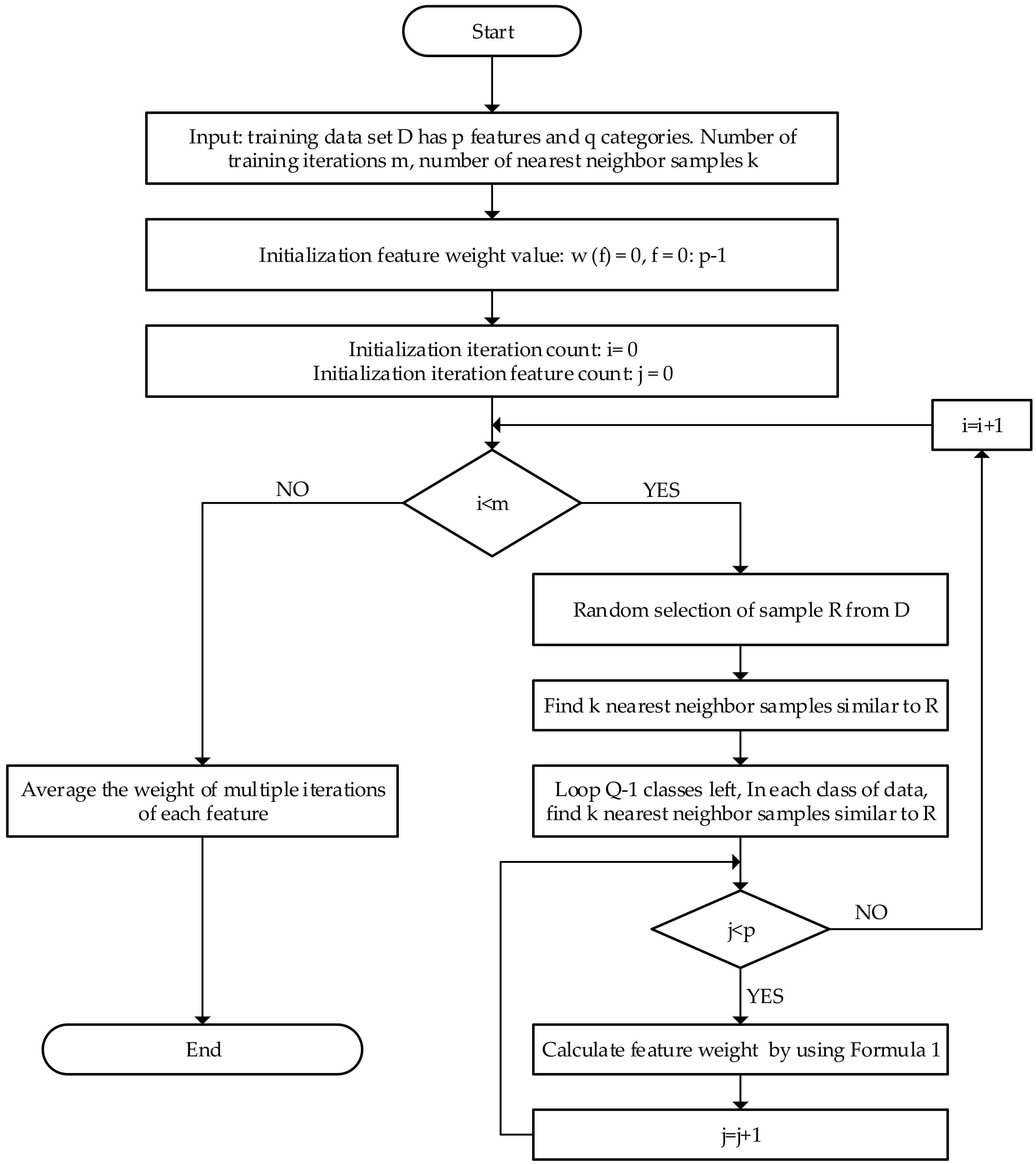
The ReliefF algorithm is an improvement on the Relief algorithm and is mainly used for feature selection of multi-class labels [18,19]. The core idea of the ReliefF algorithm is to judge the correlation between observed features and categories by calculating the weight of each feature. The larger the weight, the more sensitive it is to multi-class classification. The specific implementation process of the algorithm is as follows: Suppose you want to sample the sample set m times, and there are n observation features in the data set. In each sampling, first select sample R randomly from the sample set, then select k nearest samples from the same kind of samples of R, then select k nearest samples from the rest of each kind of samples, and then use Equation (1) to calculate the weight of each feature circularly. Since m times are sampled, the above process iterates m times, and finally gets the average weight of each feature. A feature subset is output by preserving the features whose weight is greater than the threshold value. The flow chart of the ReliefF algorithm is shown in Figure 1.

The equation to calculate the weight of each feature circularly is shown as:

$$\begin{array}{l}\mathrm{W}{(T)}_i=W{(T)}_{i-1}-{\displaystyle \sum _{\mathrm{j}=1}^{k}diff(T,R,H_j)}/(mk)\\ +{\displaystyle {\sum }_{C\ne class(R)}}[\frac{p(C)}{1-p(class(R))}{\displaystyle \sum _{j=1}^{k}diff(T,R,M_j(C))}]/(mk)\end{array},$$

(1)

where $\mathrm{W}{(T)}_i$ represents the weight of the t-th feature in the i-th iteration, and the initial value is 0, $H_j$ represents k nearest neighbor samples of the same kind as R, $M_j(C)$ represents k nearest neighbor samples different from R, $p(C)$ is the probability of class C, $diff(T,R,H_j)$ represents the distance between sample R and sample $H_j$ on feature T, and $diff(T,R,M_j(C))$ represents the distance between sample R and sample $M_j(C)$ on feature T. The distance equation is shown as:

$$diff(T,R_1,R_2)=\left\{\begin{array}{l}\frac{\left|R_1[T]-R_2[T]\right|}{\max (T)-\min (T)};ifTiscontinuous\\ \\ 0;ifTisdiscreteand{R}_1[T]=R_2[T]\\ 1;ifTisdiscreteand{R}_1[T]\ne R_2[T]\end{array}\right..$$

(2)

2.2. The Principle of the XGBoost Algorithm

The XGBoost algorithm was originally proposed by Chen Tianqi in 2016. It is a large-scale parallel machine learning algorithm based on Integrated Learning [20]. The XGBoost algorithm is a combination of multiple Classification and Regression Tree (CART) based on boosting integrated learning ideas.

The CART is a kind of decision tree algorithm that can be used for both classification and regression. The generation of a CART is the process of recursively constructing a binary decision tree. Assuming that the characteristics of the data set are a, b, and c, the binary tree constructed by a CART is shown in Figure 2.

The CART uses a top-down design method. Each iteration loop selects a feature attribute to be forked until it cannot be forked again. In the process of a CART construction, there are two major issues. The first is how to choose the best bifurcation feature attribute, and the second is how to get the best prediction score.

There are two main ideas of boosting learning. The first point is that the selection of training set in each iteration is related to the learning results of the previous rounds; the second point is that it changes the data distribution by updating the weight of each sample in each iteration. There are two steps to train the classifier by using boosting learning. The first step is to learn each weak classifier step by step. The final strong classifier is composed of all the classifiers generated step by step. The second step is to change the weight of each sample according to the result in the previous step.

The main idea of the XGBoost algorithm is to build a classification regression tree by using all the features in the data set. Each time a classification feature node is added, it is to learn a new function, and use the learning results to fit the last prediction residual; after the training, it is a K tree containing K classification feature nodes. For the prediction score of each sample, we need to find all the corresponding leaf nodes according to the characteristics of the sample, and the sum of the scores of all the leaf nodes is the prediction value of the sample.

The XGBoost is integrated by multiple CART trees. The model expression is shown as:

$${\widehat{y}}_{\mathrm{i}}={\displaystyle \sum _{k=1}^K{f}_k(x_i)}\hspace{1em}\hspace{1em}{f}_k\in F,$$

(3)

where ${\widehat{y}}_i$ is the predicted value; $x_i$ is the sample of i-th input; $K$ is the total number of trees, $F$ represents the function space of decision tree (all cart trees), and $f_k$ represents a function in function space $F$. In order to better learn the aforementioned model, it is necessary to minimize the objective function. The objective function of the XGBoost algorithm is shown as:

$$Obj(\mathsf{\Phi })={\displaystyle \sum _{i=1}^{n}l({\widehat{y}}_i,y_i)}+{\displaystyle \sum _{k=1}^K\mathsf{\Omega }(f_k)}.$$

(4)

The objective function consists of two parts. The first part is the loss function used to measure the difference between the predicted value and the true value. The second part is the penalty term of the model complexity, it is represented by $\mathsf{\Omega }$. The expansion of $\mathsf{\Omega }$ is shown in Equation (5):

$$\mathsf{\Omega }(f)=\gamma T+\frac{1}{2}\lambda ||\omega |{|}^2,$$

(5)

where $\gamma$ represents the regularization parameter of leaf number, which is used to restrain the node from further splitting; $\lambda$ represents the regularization parameter of leaf weight, which is used to prevent the node score from being too large; $T$ represents the number of leaf nodes; $\omega$ represents the score of leaf nodes.

In the process of constructing a CART, the XGBoost algorithm solves the problem of bifurcation feature selection through greedy thoughts on the one hand, and solves the problem of obtaining prediction scores by optimizing the objective function on the other. When selecting the bifurcation feature, the XGBoost algorithm uses the “greedy strategy” to select the feature with the smallest target function value at the current moment as the bifurcation feature by enumerating the target function value. When calculating the predicted score of each leaf node, the XGBoost calculates the minimum value of the objective function, and the minimum value point is the predicted score of the leaf node.

Because the XGBoost algorithm uses a gradient boosting strategy internally, when constructing a classification regression tree, not all the trees are obtained at once, but a new tree is added each time, and the previous test results are continuously patched while adding new trees. Assume that the predicted value after generating t trees is ${\widehat{y}}_i{}^{(t)}$. The derivation process is shown as:

$$\left\{\begin{array}{l}{\widehat{y}}_i{}^{(0)}=0\\ {\widehat{y}}_i{}^{(1)}=f_1(x_i)={\widehat{y}}_i{}^{(0)}+f_1(x_i)\\ {\widehat{y}}_i{}^{(2)}=f_1(x_i)+f_2(x_i)={\widehat{y}}_i{}^{(1)}+f_2(x_i)\\ ⋮\\ {\widehat{y}}_i{}^{(t)}={\displaystyle \sum _{k=1}^t{f}_k(x_i)}={\widehat{y}}_i{}^{(t-1)}+f_t(x_i)\end{array}\right..$$

(6)

Therefore, the objective function of each layer is shown as:

$$\begin{array}{l}{\mathrm{Obj}}^{(t)}={\displaystyle \sum _{i=1}^{n}l({\widehat{y}}_i{}^{(t)},y_i)}+{\displaystyle \sum _{i=1}^t\mathsf{\Omega }(f_i)}\\ ={\displaystyle \sum _{i=1}^{n}l({\widehat{y}}_i{}^{(t-1)}+f_t(x_i),y_i)}+\mathsf{\Omega }(f_t)\end{array},$$

(7)

The purpose of Equation (7) is to find a way to minimize the objective function. The Taylor expansion of the objective function at $f_t=0$ is shown in Equation (8):

$${\mathrm{Obj}}^{(t)}={\displaystyle \sum _{i=1}^n\left[l({\widehat{y}}_i{}^{(t-1)},y_i)+g_i{f}_t(x_i)+\frac{1}{2}{h}_i{f}_t^2(x_i)\right]}+\mathsf{\Omega }(f_t),$$

(8)

where $g_i={\partial }_{{\widehat{y}}_i{}^{(t-1)}}l(y_i,{\widehat{y}}_i^{(t-1)})$ is the first derivative and $h_i={\partial }_{{\widehat{y}}_i^{(t-1)}}^{2}l(y_i,{\widehat{y}}_i^{(t-1)})$ is the second derivative. Delete the constant term and get the objective function of step t as shown as:

$${\mathrm{Obj}}^{(t)}={\displaystyle \sum _{i=1}^n\left[g_i{f}_t(x_i)+\frac{1}{2}{h}_i{f}_t^2(x_i)\right]}+\mathsf{\Omega }(f_t).$$

(9)

Put $\mathsf{\Omega }(f_t)$ into Equation (9) and the object function is shown as:

$$\begin{array}{l}{\mathrm{Obj}}^{(t)}={\displaystyle \sum _{i=1}^n\left[g_i{w}_q(x_i)+\frac{1}{2}{h}_i{w}_q^2(x_i)\right]}+\gamma T+\frac{1}{2}\lambda {\displaystyle \sum _{j=1}^T{w}_j^2}\\ ={\displaystyle \sum _{j=1}^T\left[G_j{w}_j+\frac{1}{2}(H_j+\lambda )w_j^2\right]}+\gamma T\end{array},$$

(10)

where $G_j={\displaystyle {\sum }_{i\in I_j}{g}_i}$, $H_j={\displaystyle {\sum }_{i\in I_j}{h}_i}$, $I_j=\left\{i|q(x_i)=j\right\}$ represents the sample set belonging to the j-th leaf node. The minimum value of the objective function of the aforementioned leaf node score $w$ can be obtained by making its derivative zero. The minimum value point is the optimal leaf node prediction score and is shown as:

$$w_j^{*}=-\frac{G_j}{H_j+\lambda }.$$

(11)

Take Equation (11) into the objective function, and the minimum value of the objective function is shown as:

$$Ob{j}^{*}=-\frac{1}{2}{\displaystyle \sum _{j=1}^T\frac{G_j^2}{H_j+\lambda }}+\lambda T.$$

(12)

3. Design of Fault Diagnosis Algorithm for Key Parts of Wind Turbine

In order to reduce and avoid the losses caused by the wind turbine shutdown, it is necessary to timely and accurately detect whether there are faults and specific fault types in the gearbox and generator of the wind turbine. Therefore, the fault diagnosis algorithm proposed in this paper is as follows.

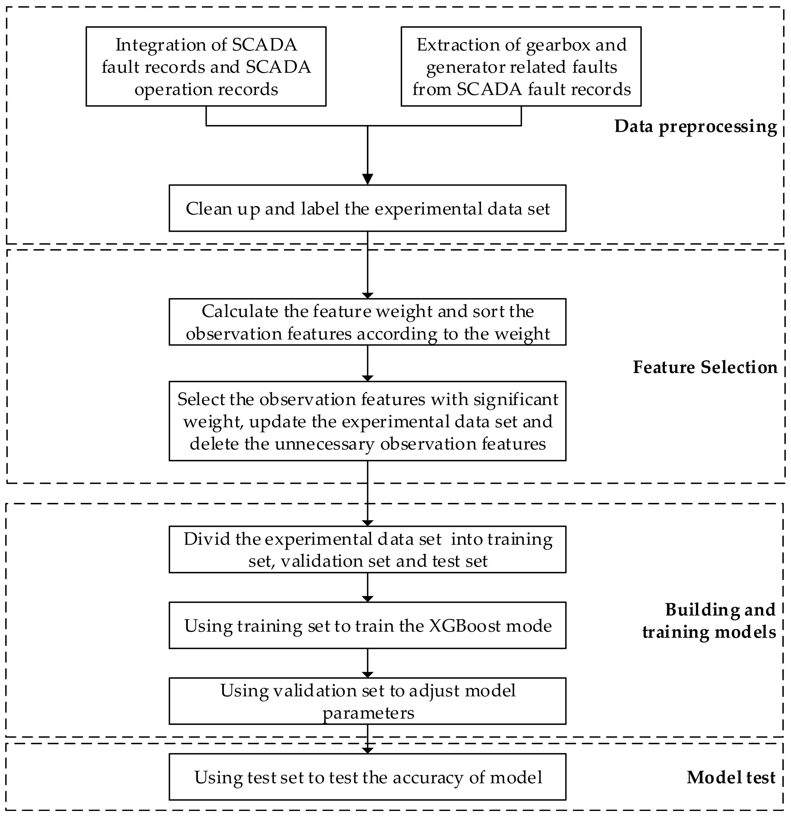
Step 1: Data acquisition and data preprocessing. First of all, we need to obtain the operation monitoring records and fault records of the SCADA system. Select relevant faults of gearbox and generator from the fault records of the SCADA system, and sort out the types of fault records. We need to find the normal data set and each type of fault data set according to the fault record and SCADA system monitoring record, and combine the normal data set and fault data set as the experimental data set. Before selecting the features of the SCADA system data, the experimental data set needs to be pre-processed, including deleting the empty data record. After data preprocessing, data categories need to be labeled. Common sequence encoding and one hot encoding can be adopted.

Step 2: Use the ReliefF algorithm to find the weight of each SCADA system observation parameter in the fault classification. Due to the imbalance of data proportion between normal data and fault data in the experimental data set, this paper adopts a stratified sampling strategy for the experimental data set in the calculation process of the ReliefF algorithm, which not only covers all the classified sample features, but also avoids the result deviation caused by the different sample data amount. Then we arrange the feature parameters calculated by the ReliefF algorithm in the order of weight from large to small, select the feature parameters that have a greater impact on the related faults of the gearbox and generator, and remove the observation features with a smaller correlation. Next, we reorganize the experimental data set according to the selected characteristic parameters.

Step 3: We divide the rearranged experimental data set into a training set, validation set and a test set. Then we use the training set to train the XGBoost multi classification model, and use the validation set to adjust the model parameters.

Step 4: Use the optimized XGBoost model to perform a fault multi-classification test on the test set data. The algorithm flow chart is shown in Figure 3.

4. Case Analysis and Result Comparison

In this paper, the information from the SCADA system recorded from 33 Vestas wind turbines in Daguangding Wind Farm in Inner Mongolia from 1 January 2019 to 1 December 2019 was used as experimental data. In order to obtain as many fault data as possible, this paper selected multiple wind turbines of the same type in the same wind farm and counted the fault types of the gearbox and generator in one year, and selected six faults shown in

Table 1. Fault type.

Number	Fault Types
1	Rotor RPM, generator RPM
2	Excessive speed of rotor
3	High temperature on generator
4	High temperature on Gen bear
5	High temperature on bear
6	Gear oil radiator overload

as the fault type set according to the frequency sequence of all fault types.

We needed to use the SCADA system operation monitoring record and fault record to get the fault data set, and then combined the normal data set to form the original data set. We first deleted the empty data in the original data set and then selected 1000 data of each type as the experimental data set. The experimental data set had a total of 7000 data. In the last, we coded the fault categories in the experimental data set. The fault code table is shown in

Table 2. Fault code.

Fault Types	Fault Code
Normal operation	1
Rotor RPM, generator RPM	2
Excessive speed of rotor	3
High temperature on generator	4
High temperature on Gen bear	5
High temperature on bear	6
Gear oil radiator overload	7

. We used the Python function library to build the ReliefF algorithm and we also used the scikit-learn function library to build the XGBoost classification model. The programming software was pycharm.

4.1. Selecting Characteristic Parameters by ReliefF

There are 42 observation characteristic parameters in the SCADA system of Vestas wind turbine. The weight values of each observation feature were obtained after calculation by the ReliefF algorithm, and the values of each observation feature were arranged as shown in

Table 3. Observed feature weights.

Features	Weights
Active setting feedback value	0.276603
Annual power generation	0.17884
Blade 1 pitch angle A	0.177146
Total generating capacity	0.170743
Gearbox inlet oil pressure	0.169514
Impeller speed	0.159299
Generator speed	0.151687
Ambient temperature	0.140054
Phase C current at grid side	0.132598
Phase A current at grid side	0.13121
Active power	0.130947
Phase B current at grid side	0.128243
Fan status reception	0.120974
Ambient wind direction	0.096194
Converter coolant inlet temperature	0.083146
Daily power loss	0.078387
Power factor	0.078157
Daily power generation	0.074917
The temperature of inverter grid-side IGBT	0.074055
Monthly power generation	0.072639
Hydraulic system oil temperature V1	0.070859
Generator stator winding temperature W1	0.068143
Generator stator winding temperature U1	0.065242
Generator stator winding temperature V1	0.064828
Daily power generation	0.063899
Generator slip ring temperature	0.062178
Converter control cabinet temperature	0.061467
Temperature of reactor 1 at converter grid side	0.057386
Phase C voltage at grid side	0.043991
Generator drive side bearing temperature	0.036021
Frequency	0.035615
Phase B voltage at grid side	0.033013
Converter controller temperature	0.032884
A-phase voltage at grid side	0.031477
Ambient wind speed	0.030492
Gearbox high speed bearing temperature	0.026052
Gearbox oil temperature	0.021837
Reactive power	0.007668
The temperature of converter rotor side L1	0.006128
The temperature of converter rotor side L3	0.005562
The temperature of converter rotor side L2	0.005536
Hydraulic system oil pressure	0.001442

according to the weight values from large to small.

Finally, we chose 27 characteristic parameters as the observation parameters of fault diagnosis. The list of selected observation parameters is shown in

Table 4. Observed features.

Number	Features
1	Active setting feedback value
2	Annual power generation
3	Blade 1 pitch angle A
4	Total generating capacity
5	Gearbox inlet oil pressure
6	Impeller speed
7	Generator speed
8	Ambient temperature
9	Phase C current at grid side
10	Phase A current at grid side
11	Active power
12	Phase B current at grid side
13	Fan status reception
14	Ambient wind direction
15	Converter coolant inlet temperature
16	Daily power loss
17	Power factor
18	Daily power generation
19	The temperature of inverter grid-side IGBT
20	Monthly power generation
21	Hydraulic system oil temperature V1
22	Generator stator winding temperature W1
23	Generator stator winding temperature U1
24	Daily power generation
25	Generator slip ring temperature
26	Converter control cabinet temperature
27	Temperature of reactor 1 at converter grid side

.

4.2. Fault Identification with XGBoost

In order to get the operation status of the wind turbine by using the SCADA system monitoring parameters, it is necessary to realize the mapping from the feature space to the state space of the wind turbine. After extracting the fault related parameters, we had to modify the original experimental data set and delete the monitoring values of unrelated items. The data set consisted of 28 columns, including 27 observation parameter columns and one status coding column. Then we needed to use the XGBoost classifier to complete the mapping from the observation parameter value to the state of the wind turbine. Finally, we were able to achieve the goal of obtaining the fault type through the value of 27 observation parameters.

We divided 70% of the experimental data into a training set, 20% into a validation set, and 10% in the test set. Then we input the training data set into the XGBoost model for fault recognition training. By constantly adjusting the parameters, we finally obtained the optimal classification model. The optimal parameters are shown in

Table 5. Parameters for extreme gradient boosting.

Parameter	Value
n estimators	200
learning rate	0.12
max dapth	5
min child weight	1
objective	Multi:softmax
num class	7
nthread	4

.

In Table 5, “n estimators” is the maximum number of trees generated and the maximum number of iterations. “learning rate” refers to the step size of each iteration, and the system default value is 0.3. If the value of “learning rate” is too large, the running accuracy will be low, and if it is too small, the running speed will be slow. “max depth” is the maximum depth of the tree. The default value is 6, which is used to control over fitting. The larger the value of “max depth”, the more specific the model learning. “min child weight” refers to the minimum sample weight required to generate a child node. If the sample weight on the newly generated child node is less than the number you specify, then the child node will not grow. “objective” is used to define learning tasks and corresponding learning objectives. The objective function selected in this paper is “multi: softmax”. The purpose of using this parameter is to let XGBoost use softmax objective function to deal with multi classification problems. “num class” refers to the number of categories in multi classification, and “nthread” refers to the number of threads opened when the program is running.

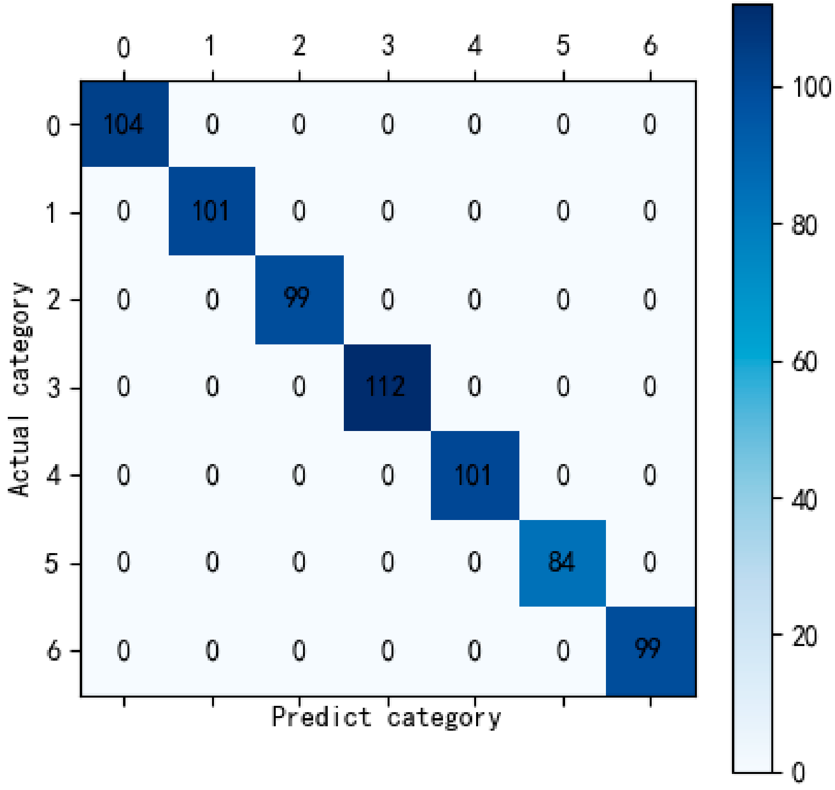
After training and parameter adjustment, we finally got a XGBoost model with better classification effect. Confusion matrix, also known as error matrix, is a standard format for precision evaluation. After inputting the test data set into the XGBoost model, we finally got the confusion matrix of the test set as shown in Figure 4.

The abscissa in Figure 4 represents the prediction category of the sample, and the ordinate represents the actual category of the sample. It can be seen from the confusion matrix that there are 700 samples in the test sample set. According to Figure 4, the predicted and actual categories of all samples are exactly the same. Through the analysis, the classification accuracy of the test set data in the XGBoost model was as high as 100%.

4.3. Comparison of Experimental Results

In order to evaluate the fault diagnosis performance of the algorithm described in this paper, we used the accuracy, macro precision ($P_{Macro}$), macro recall ($R_{Macro}$) and macro F1-Score ($F_{1,Macro}$) of the final classification results as the evaluation indexes. Accuracy is the most common evaluation index. Accuracy refers to the number of correctly classified samples divided by all samples. Generally speaking, the higher the accuracy, the better the classifier performance. The precision, recall and F1-Score are the evaluation indexes of the binary classification model, which are now used in the evaluation of the multi classification model. We treat each category individually as “positive” and all other categories as “negative”. Precision refers to the ratio between the number of samples that are predicted to be positive and the number of samples actually positive. Recall refers to the ratio between the number of samples predicted as positive and the actual number of samples in this category. F1-Score is a classification accuracy of the model which is obtained by combining the precision and recall. Macro precision is the average value of precisions in multiple binary classification models. Macro recall is the average value of recalls in multiple binary classification models. Macro F1-Score is the average of all F1-Score values. In order to prove the superiority of the algorithm described in this paper, we used the test set to carry out the following two experiments.

Experiment 1: “ReliefF + Support Vector Machine based on radial basis kernel function (rbf-SVM)” algorithm. Support Vector Machine (SVM) algorithm was originally designed for the binary classification problem. The basic principle of SVM is to find the hyperplane with the maximum interval in feature space. In the face of multi classification tasks, SVM can use different mapping kernel functions to map the feature points that are difficult to be separated in low dimension to high dimension, and create a hyperplane to separate them in high dimension. After the completion of the model construction, the optimal parameters selected through repeated adjustment are: “C = 3”, “kernel = RBF”, “gamma = 0.01”, “decision_function_shape = ovr”. The value of “C” is the penalty coefficient, which refers to the tolerance of error. The higher the value of “C”, the more intolerable the error is, and it is easy to over fit. The smaller the value of “C”, the less fitting it is. The value of “kernel” is used to set the kernel function of the model. “Gamma” is a parameter that comes with the RBF function when it is selected as the kernel. The value of gamma determines the distribution of data mapped to the new feature space. The larger the value of gamma, the less the support vector. The smaller the value of gamma, the more the support vector. The number of support vectors affects the speed of training and prediction.

Experiment 2: “ReliefF + Adaptive Boosting (AdaBoost)” algorithm. AdaBoost is also a kind of boosting algorithm. AdaBoost’s core idea is to train different classifiers (weak classifiers) for the same training set, and then combine these weak classifiers to form a stronger final classifier. There are two kinds of weights in AdaBoost: sample weight and classifier weight. In the iterative process, the sample weight of the wrong samples will increase, and the next classification will pay more attention to the wrong samples. Each iteration will produce a classifier, each classifier has a classifier weight, and finally the weak classifier will be combined according to the classifier weight to form a strong classifier. After the completion of the ReliefF + AdaBoost model, the final optimization parameters of the model are: “n estimators = 500”, “learning rate = 1.0”. The value of “n estimators” is the maximum number of iterations. The value of “learning rate” is the model’s learning rate, which refers to the step length of each iteration.

The results of the algorithm described in this paper and two comparative experiments is shown in Figure 4.

In Figure 5, the height of the red column represents the accuracy of the aforementioned three experiments; the height of the blue column represents the macro precision of every experiment; the height of the green column represents the macro recall of the aforementioned three experiments; the height of the purple column represents the macro F1-Score of the experiments. From Figure 5, we can clearly see that the algorithm described in this paper is the most accurate no matter which evaluation standard is used.

In conclusion, using “ReliefF + XGBoost” algorithm for fault diagnosis has the highest accuracy and the best effect.

5. Conclusions

In this paper, a solution for fault diagnosis of a wind turbine is proposed. In the algorithm described in this paper, we take the historical data of SCADA system as the input, use the ReliefF algorithm to select the fault related parameters, then use the fault related data to establish a fault diagnosis model, and finally send the real-time running wind turbine’s data to the XGBoost model to complete the fault diagnosis. The experimental results showed that the “ReliefF + XGBoost” algorithm could realize fault diagnosis, and the algorithm had the advantage of high precision as verified through comparison.

References

- Xiaoli, L.; Chuanglin, F. Wind energy resources distribution and spatial differences of wind power industry in China. In Proceedings of the 2007 Non-Grid-Connected Wind Power Systems—Wind Power Shanghai 2007—Symposium on Non-Grid-Connected Wind Power, NGCWP 2007, Shanghai, China, 2 November 2007; pp. 182–197. [Google Scholar]
- Zhang, Z.; Verma, A.; Kusiak, A. Fault Analysis and Condition Monitoring of the Wind Turbine Gearbox. IEEE Trans. Energy Convers. 2012, 27, 526–535. [Google Scholar] [CrossRef]
- Ribrant, J.; Bertling, L.M. Survey of failures in wind power systems with focus on Swedish wind power plants during 1997–2005. IEEE Trans. Energy Convers. 2007, 22, 167–173. [Google Scholar] [CrossRef]
- Pinar Perez, J.M.; Garcia Marquez, F.P.; Tobias, A.; Papaelias, M. Wind turbine reliability analysis. Renew. Sustain. Energy Rev. 2013, 23, 463–472. [Google Scholar] [CrossRef]
- Spinato, F.; Tavner, P.J.; Van Bussel, G.J.W.; Koutoulakos, E. Reliability of wind turbine subassemblies. Iet Renew. Power Gener. 2009, 3, 387–401. [Google Scholar] [CrossRef] [Green Version]
- McMillan, D.; Ault, G.W. Condition monitoring benefit for onshore wind turbines: Sensitivity to operational parameters. IET Renew. Power Gener. 2008, 2, 60–72. [Google Scholar] [CrossRef]
- Guo, P.; Infield, D.; Yang, X. Wind turbine gearbox condition monitoring using temperature trend analysis. Proc. Chin. Soc. Electr. Eng. 2011, 31, 129–136. [Google Scholar]
- Yin, H.; Jia, R.; Ma, F.; Wang, D. Wind Turbine Condition Monitoring based on SCADA Data Analysis. In Proceedings of the 3rd IEEE Advanced Information Technology, Electronic and Automation Control Conference, IAEAC 2018, Chongqing, China, 12–14 October 2018; pp. 1101–1105. [Google Scholar]
- Gomez, M.J.; Castejon, C.; Corral, E.; Garcia-Prada, J.C. Analysis of the influence of crack location for diagnosis in rotating shafts based on 3 x energy. Mech. Mach. Theory 2016, 103, 167–173. [Google Scholar] [CrossRef]
- Tang, B.; Liu, W.; Song, T. Wind turbine fault diagnosis based on Morlet wavelet transformation and Wigner-Ville distribution. Renew. Energy 2010, 35, 2862–2866. [Google Scholar] [CrossRef]
- Wang, Y.; Ma, X.; Qian, P. Wind Turbine Fault Detection and Identification Through PCA-Based Optimal Variable Selection. IEEE Trans. Sustain. Energy 2018, 9, 1627–1635. [Google Scholar] [CrossRef] [Green Version]
- Ruiz, M.; Mujica, L.E.; Alferez, S.; Acho, L.; Tutiven, C.; Vidal, Y.; Rodellar, J.; Pozo, F. Wind turbine fault detection and classification by means of image texture analysis. Mech. Syst. Signal Process. 2018, 107, 149–167. [Google Scholar] [CrossRef] [Green Version]
- Pozo, F.; Vidal, Y.; Salgado, O. Wind turbine condition monitoring strategy through multiway PCA and multivariate inference. Energies 2018, 11. [Google Scholar] [CrossRef] [Green Version]
- Liang, Y.; Fang, R. An online wind turbine condition assessment method based on SCADA and support vector regression. Autom. Electr. Power Syst. 2013, 37, 7–12. [Google Scholar] [CrossRef]
- Bangalore, P.; Tjernberg, L.B. An artificial neural network approach for early fault detection of gearbox bearings. IEEE Trans. Smart Grid 2015, 6, 980–987. [Google Scholar] [CrossRef]
- Wang, L.; Zhang, Z.; Long, H.; Xu, J.; Liu, R. Wind Turbine Gearbox Failure Identification with Deep Neural Networks. IEEE Trans. Ind. Inform. 2017, 13, 1360–1368. [Google Scholar] [CrossRef]
- Vidal, Y.; Pozo, F.; Tutiven, C. Wind turbine multi-fault detection and classification based on SCADA data. Energies 2018, 11. [Google Scholar] [CrossRef] [Green Version]
- Kononenko, I. Estimating attributes: Analysis and extensions of RELIEF. In Proceedings of the European Conference on Machine Learning, ECML 1994, Catania, Italy, 6–8 April 1994; pp. 171–182. [Google Scholar]
- Robnik-ikonja, M.; Kononenko, I. Theoretical and Empirical Analysis of ReliefF and RReliefF. Mach. Learn. 2003, 53, 23–69. [Google Scholar] [CrossRef] [Green Version]
- Chen, T.; Guestrin, C. XGBoost: A scalable tree boosting system. In Proceedings of the 22nd ACM SIGKDD International Conference on Knowledge Discovery and Data Mining, KDD 2016, San Francisco, CA, USA, 13–17 August 2016; pp. 785–794. [Google Scholar]
- Kira, K.; Rendell, L.A. Feature selection problem: Traditional methods and a new algorithm. In Proceedings of the Tenth National Conference on Artificial Intelligence—AAAI-92, San Jose, CA, USA, 12–16 July 1992; pp. 129–134. [Google Scholar]
- Xie, Y.; Li, D.; Zhang, D.; Shuang, H. An improved multi-label relief feature selection algorithm for unbalanced datasets. In Proceedings of the 2nd International Conference on Intelligent and Interactive Systems and Applications, IISA 2017, Beijing, China, 17–18 June 2017; pp. 141–151. [Google Scholar]
Figure 1.
The flow chart of the ReliefF algorithm.
Figure 2.
Classification and Regression Tree (CART).
Figure 3.
Algorithm flow chart.
Figure 4.
The confusion matrix.
Figure 5.
The result of the fault classification algorithm.