Magnetic Resonance-Electrical Properties Tomography by Directly Solving Maxwell’s Curl Equations

Abstract

Magnetic Resonance-Electrical Properties Tomography (MR-EPT) is a method to reconstruct the electrical properties (EPs) of bio-tissues from the measured radiofrequency (RF) field in Magnetic Resonance Imaging (MRI). Current MR-EPT approaches reconstruct the EP profile by solving a second-order partial differential wave equation problem, which is sensitive to noise and can induce large reconstruction artefacts near tissue boundaries and areas with inaccurate field measurements. In this paper, a novel MR-EPT approach is proposed, which is based on a direct solution to Maxwell’s curl equations. The distribution of EPs is calculated by iteratively fitting the RF field calculated by the finite-difference-time-domain (FDTD) technique to the measured values. To solve the time-consuming problem of the iterative fitting, a graphics processing unit (GPU) is used to accelerate the FDTD technique to process the field calculation kernel. The new EPT method was evaluated by investigating a numerical head phantom, and it was found that EP values can be accurately calculated and were relatively insensitive to simulated RF field errors. The feasibility of the proposed method was further validated using phantom-based experimental data collected from a 9.4 Tesla (T) Magnetic Resonance Imaging (MRI) system. The results also indicated that more accurate EP values could be reconstructed from the new method compared with conventional methods. Moreover, even in the absence of phase information of the RF field, the proposed approach is still capable of offering robust EPT solutions, thus having improved practicality for potential clinical applications.

1. Introduction

Magnetic Resonance-Electrical Properties Tomography (MR-EPT) is an imaging technique which maps the electrical properties (permittivity and conductivity) of a subject by analyzing the radiofrequency (RF) magnetic field measured during an MR scan. This technique has shown promise for clinical diagnosis and interests in ultra-high field Magnetic Resonance Imaging (MRI), because of its potential in the evaluation of patient-specific absorption rate (SAR) [1]. MR-EPT has also shown promise for clinical diagnosis and guiding the treatment of malignant tissues [2,3] and improving the patient-specific electromagnetic (EM) modelling of hyperthermia [4]. The concept of MR-EPT was introduced by Haacke et al. in 1991 [5], and Wen et al. [6] verified this concept through experiments in 2003. The initial development of MR-EPT was based on the utilization of the Helmholtz equation, in which the permittivity and conductivity were assumed constant (also known as the “local homogeneity assumption” (LHA)) [7,8]. The methods based on this LHA have been found to be sensitive to noise, and severe distortions at the boundaries of different tissues may occur [9,10]. To reduce the noise amplification in the utilization of second-order derivatives, several methods have been proposed. Additional regularization terms were added to solve the EPT inverse problem [11,12], the Laplacian operator was replaced with a surface integral [8,13], the k-space data were weighted properly [14], and the region of interest (ROI) was expanded with more voxels [15]. Numerical and experimental results in References [11,12,13,14,15] demonstrated that these methods improved the noise robustness but failed to correct the edge artefacts caused by the LHA. To eliminate these edge artefacts, a new set of partial differential equations (PDE) was introduced [16,17,18,19,20,21]. In References [16,17,18], the special gradients of EPs were considered as unknown variables in the PDE, which were resolved by using multi-channel parallel transmit coils. In this scheme, the condition number of the constructed PDE was reduced, and the inverse solution was thus improved. An alternative method to resolve the unknown EP variables is to transform the PDE into a linearly regularized system and search for its global solution [19,20,21]. Although the methods in References [16,17,18,19,20,21] have been tested in experiments, it is noteworthy that the EP reconstructions were implemented in an inverse process, in which the solution robustness could be weakened by the ill-conditioned property of the linear system. For these reasons, the development of new EPT approaches without the involvement of second-order PDE (i.e., Laplacian-operator free) is of interest.

Recently, EP reconstruction in MRI has been alternatively investigated using the integral equations (IE). The IE-based EPT methods rely on a global convolution between the Green function and the contrast source [22,23,24,25,26] With the integral of global convolution, the noise robustness is theoretically improved in those IE-based methods. However, the development of IE-EPT is still at an initial stage and facing several practical problems. The technical problems include the requirement of the estimation of the incident electromagnetic fields, low spatial resolution, the accuracy issue associated with the use of the free-space Green function to construct the contrast source and the necessity of using global convolution.

In this paper, a novel MR-EPT method is proposed. In the presented method, the EP reconstruction was achieved by directly solving Maxwell’s equations [27,28]. That is, the first-order PDE was numerically solved by using an in-house finite-difference-time-domain (FDTD) method with the graphics processing unit (GPU)-based acceleration. The unknown EP profile was involved in the FDTD kernel solver, and an optimization procedure was performed to refine the EP profile to minimize the difference between the calculated and measured transmit magnetic fields ($B_1^{+}$). To demonstrate the feasibility of the proposed EPT method, human brain simulation and phantom-based experimental studies have been carried out, and EP reconstruction results were compared with conventional approaches.

2. Theory and Method

Figure 1 shows the frameworks of different EPT methods. Conventional differential-based methods (Figure 1a,b) rely on inverse processes involving second-order differential kernels in the EP reconstruction. In the proposed approach (Figure 1d), a forward process is used, which investigates the relationship between the EPs and the amplitude of $B_1^{+}$ data, and only involves first-order derivative; thus, it is Laplacian-operator free. Details of differential equations for the description of radiofrequency problems in MRI can be found in the literature [18]. When the other conditions are pre-known (such as the structures of the coil and subject), the amplitude of the $B_1^{+}$ field is mainly determined by the EPs of the imaging subject. Therefore, it is possible to optimize the EPs during the forward process so that the calculated amplitude of the $B_1^{+}$ field can match the measured one. The efficiency and accuracy of this approach rely on the forward solver and the optimizer. Because the EPs are iteratively optimized during each forward process, an efficient forward EM solver is required to achieve a practical solution. As opposed to conventional methods, the proposed method calculates the EP values using the full set of magnetic field components available from the EM solver, without neglecting the z-component of the magnetic field ($B_z$) [18]. The details of the forward solver and optimization process are given below.

2.1. GPU-Accelerated FDTD Solver

The in-house built FDTD solver [29] was constructed based on the differential form of the Maxwell equations (ME). As the first-order central differential scheme was used to implement the partial derivatives in the ME numerically, the noise effects were only amplified in the first-order rate, which was more robust than conventional EPT methods based on second-order wave equation. In the FDTD computational domain, a uniform mesh was used to discretize the subject-coil space, and specific cell sizes were problem-dependent. The calculation volume was truncated with perfectly matched layers (PML). The PML was composed of 8 to 10 layers, and the conductivities of each layer were calculated based on the method presented in Reference [30].

In the FDTD solver, the vector forms of the electric and magnetic fields were calculated for the evaluation of $\left|B_1^{+}\right|=\left|B_x+i{B}_y\right|/2$ [31]. Here, as Maxwell’s curl equations state, the calculated $\left|B_1^{+}\right|$ fields were a function of EPs of the imaged subject. For more details about the in-house developed FDTD solver, please refer to our previous work [29].

In the constructed optimization problem, the forward process was implemented in each iteration step; thus the FDTD solver was required to run efficiently for the evaluation of the $\left|B_1^{+}\right|$ field. To this end, a GPU-accelerated FDTD solver [29] was applied to the proposed EPT solution procedure. In this study, a 12-rung birdcage coil was modelled as an EM source and loaded with a subject (phantom or head), as shown in Figure 2. A perfect electric conductor (PEC) was placed around the birdcage coil to simulate the RF shield, and PML boundary conditions were placed at the top and bottom of the computation domain. In the FDTD simulation, Maxwell’s curl equations are approximated with Yee’s ‘leap-frog’ finite-difference algorithm, and the entire computational space is translated from standard Cartesian space to Yee-cell space, where the FDTD equations exhibit inherent strong parallelism. At each Yee-cell, this parallelism permits the simultaneous calculation of magnetic and electric field components in both space and time domains. The explicit field updating procedure was easily implemented in multiple, synchronized threads within the parallel-computing framework of a GPU. In this work, all computations have been executed on an Intel Xeon CPU E5-2680 V2 @ 2.80 GHz (128 GB RAM) equipped with an NVIDIA TITAN V GPU (12 GB RAM, 5120 CPUs, and 1455 MHz clock frequency) and more details about the GPU-FDTD computing can be found in Reference [29].

2.2. Optimization

EPs were estimated through an iterative optimization procedure. The optimization variables (EPs) are ${\mathit{x}}_{\mathrm{EP}}=\left[{\mathit{\epsilon }}_{\mathrm{tissue}}{\mathit{\sigma }}_{\mathrm{tissue}}\right]$, that is, the permittivity and conductivity values of each voxel of the imaging subject. Using the developed FDTD solver described in Section 2.1, the tissue dielectric properties variable ${\mathit{x}}_{\mathrm{EP}}$ were mapped to the $B_1^{+}$ field as:

$$B_1^{+}={ℱ}_{\mathrm{FDTD}}\left({\mathit{x}}_{\mathrm{EP}}\right),$$

(1)

where ${ℱ}_{\mathrm{FDTD}}$ denotes the FDTD process.

Then, a cost function which describes the residual between the mapped $B_1^{+}$ fields and the measured $B_1^{+}$ field can be built as:

$$C={\Vert \left|B_1^{+}\right|-\left|B_{1;meas}^{+}\right|\Vert }_2,$$

(2)

Therefore, an unconstrained optimization problem which aims to minimize the cost function can be formed as:

$$\underset{\mathit{x}}{\min }{\Vert \left|{ℱ}_{\mathrm{FDTD}}\left({\mathit{x}}_{\mathrm{EP}}\right)\right|-\left|B_{1;meas}^{+}\right|\Vert }_2,$$

(3)

The problem in Equation (3) can be efficiently solved by using optimization methods such as quasi-Newton or trust-region techniques. The EPs of the imaging subject can be obtained after the optimum ${\mathit{x}}_{\mathrm{EP}}$ is found from Equation (3).

In this work, the genetic algorithm (GA, standard MATLAB function) was used to find the optimal solution of ${\mathit{x}}_{\mathrm{EP}}$. In the optimization procedure, an initial EP distribution denoted as ${\mathit{x}}_{\mathbf{O}}$ was set based on the LHA. Inside the uniform region, the EP distribution was directly derived from the LHA-based result. On the tissue boundaries, average EPs of the neighboring tissues were used. This operation avoided the boundary artifacts in the LHA-based results. The variable range in the GA was set as ${\mathit{x}}_{\mathbf{O}}\pm 0.3{\overline{\mathit{x}}}_{\mathbf{O}}$, where ${\overline{\mathit{x}}}_{\mathbf{O}}$ is the mean value of ${\mathit{x}}_{\mathbf{O}}$. Alternatively, the initial EPs of each tissue can be set based on the data from Reference [32], and the variable range was set as ${\mathit{x}}_{\mathbf{O}}\pm 0.3{\mathit{x}}_{\mathbf{O}}$, where ${\mathit{x}}_{\mathbf{O}}$ are the reported values in Reference [33]. The GA-based optimization was implemented to satisfy one of the following stop criteria: (1) the fitness, $C$, was less than the expected fitness (least-square residual error), $C_{\mathrm{desired}}$, and (2) the number of iterations exceeds certain pre-set limits, $N_{\mathrm{desired}}$. Once condition (1) or (2) was satisfied, the optimization process could be terminated. The parameter setup of $C_{\mathrm{desired}}$ and $N_{\mathrm{desired}}$ is problem-dependent. In this study, it was observed that the variation of residual error was negligible after 50 iterations, and when it reached a value of around ${10}^{-3}$. Therefore, we chose $C_{\mathrm{desired}}$ and $N_{\mathrm{desired}}$ as ${10}^{-3}$ and 100, respectively.

The iterative optimization procedure is implemented in MATLAB (R2015a, 64 bits, The MathWorks, Inc., Natick, MA, USA).

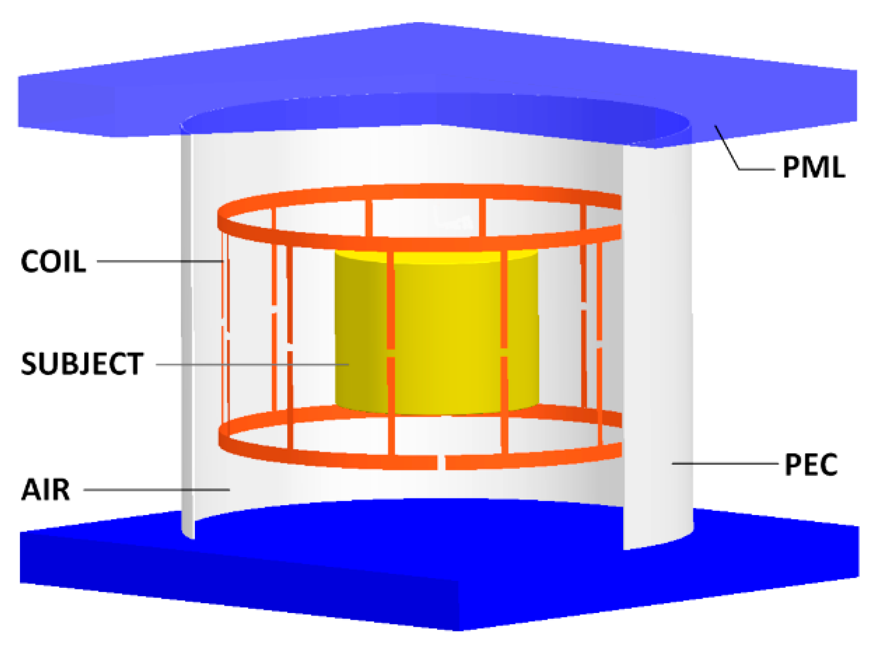
2.3. Simulation Study

The proposed EPT method was first evaluated using a simple phantom. The phantom was composed of an inner compartment with a diameter of 15 mm and an outer compartment with a diameter of 40 mm. The height of the inner and outer compartments was 50 mm. The relative permittivity for the inner and outer compartments was 78.5, and the conductivities were 0.43 S/m and 0.78 S/m, respectively. After the phantom evaluation, the head of the realistic human model Duke, from the virtual family [32], was used to study the proposed EPT method. The initial model resolution of 1 mm³ was re-meshed as 2 mm³, as a trade-off between accuracy and computational efficiency of the forward solver. The electrical properties of the brain tissues at 298 MHz (the operating frequency of 7T MRI) were determined based on the reports from Reference [33]. The head model was placed at the center of the coil (Figure 2). To assess the noise robustness of the proposed method, white Gaussian noise (GWN) was added to the simulated $B_1^{+}$ field data to achieve signal-to-noise ratios (SNR) between 15 and 55 dB [34].

2.4. Experimental Setup

To evaluate the practicality of the proposed EPT method, a phantom-based experiment at 9.4T preclinical MRI system (BioSpec 94/30 USR, Bruker, Germany) located at the Centre for Advanced Imaging, the University of Queensland, was conducted. A Bruker birdcage coil (Øouter/Øinner = 112/86 mm) was used to acquire images and the $B_1^{+}$ field. The phantom described in Section 2.3 was fabricated, with conductivities of 0.43 S/m and 0.78 S/m for the inner and outer compartments respectively, and permittivity of 78 for both compartments. The two compartments were separated by a wall (thickness = 2 mm) made of acrylic material. The EPs of the liquid solution were measured using a dielectric probe (Kit DAK-12, SPEAG Ltd., Zurich, Switzerland). The probe uncertainty and temperature-associated variation in dielectric properties were 3.3% and 2%, respectively. After careful calibration, the total measurement error can be considered less than 6.6%. The aqueous solutions consist of distilled water, NaCl, and CuSO4∙5H2O with mass ratios of 100:0.18:0.025 and 100:0.5:0.025, respectively.

Figure 3 shows the phantom and its cross-section, acquired with a gradient echo sequence. Two MR images with flip angles equal to 45° and 90° were obtained by using the fast low-angle shot (FLASH) sequence (echo time (TE) equals 5 ms and repetition time (TR) equals 5000 ms). The field-of-view in the experiment was set to 48 × 48 × 48 mm, and a 0.5 mm isotropic resolution was used in the image acquisition. The double-angle-method (DAM) [35,36] was applied to calculate the amplitude of the $B_1^{+}$ field, while the phase was calculated by using the transceive phase assumption (TPA) [6,37]. To implement the TPA, two images with different TEs (TE1 = 2.5 ms and TE2 = 3.5 ms) were used to estimate the phase difference due to the inhomogeneous $B_{\mathrm{o}}$ field. Another two images, generated using identical TE/TR but reversed gradient directions, were used to cancel the gradient-induced phase (e.g., eddy current) [6]. It should be noted that the $B_1^{+}$ phase was not used in the EP reconstruction but only for the purpose of evaluating the accuracy of the forward solver, as illustrated in the following section.

3. Results

3.1. Simulation Results

The simple phantom described in Section 2.3 was first used to evaluate the performance of the proposed EPT method. To implement the FDTD calculation, the Yee-cell size was 1 mm, and the entire computational domain was divided into D_x × D_y × D_z = 112 × 112 × 112 ≈ 1,404,928 cells. Each GPU-FDTD iteration time was approximately 18 seconds, and the total time for the optimization was around 30 min. In the evaluation, six different noise levels were added to the simulated $B_1^{+}$ field. As shown in

Table 1. Reconstructed EPs of the phantom (based on simulated data).

SNR	Inner		Outer
	εr	σ(S/m)	εr	σ
Target	78.5	0.43	78.5	0.78
Noise-free	78	0.4309	78	0.7784
SNR = 15	77	0.4428	79	0.7644
SNR = 25	77	0.4212	78	0.7918
SNR = 35	78	0.4278	78	0.7843
SNR = 45	78	0.4326	78	0.7762
SNR = 55	78	0.4322	78	0.7824

SNR: signal-to-noise ratio. σ in S/m.

, the EPs can be retrieved with high accuracy using the proposed approach, even under an extreme scenario in which the SNR level declined to 15 dB (the lowest SNR level used in current MR-EPT numerical evaluations was 35 dB). The maximum errors were 3% and 0.63% for the permittivity and conductivity reconstruction, respectively. These results show the strong robustness of the method to noise.

Following the simple phantom evaluation, the numerical head model, as described in Section 2.3, was used to assess the performance of the proposed EPT method. The target and reconstructed EP profiles are shown in Figure 4. It can be seen that accurate EPs can be retrieved by using the proposed EPT method.

To further illustrate the effectiveness of the new method, the traditional algorithm based on LHA and a recently developed EPT solution using a modified Finite-Difference (mFD) scheme [18] were both used for comparison. As a recently developed second-order differential equation-based approach, the mFD approach is a good candidate for comparison between the conventional EPT method with the proposed one. The root-mean-square-error (RMSE) [16] was used to evaluate the performance quantitatively, and the corresponding results are shown in Figure 5. It can be seen from this figure that the new EPT method achieved significantly better results than those from compared methods across SNR levels from 15 to 55 dB. In the extreme case, in which the SNR level was 15 dB, both comparison methods obtained RMSE values larger than 1.5 for the permittivity reconstruction and 1.2 for the conductivity reconstruction. However, the proposed method was capable of retrieving more accurate EP’s values with an RMSE less than 0.2 for both the permittivity and conductivity for all SNR levels.

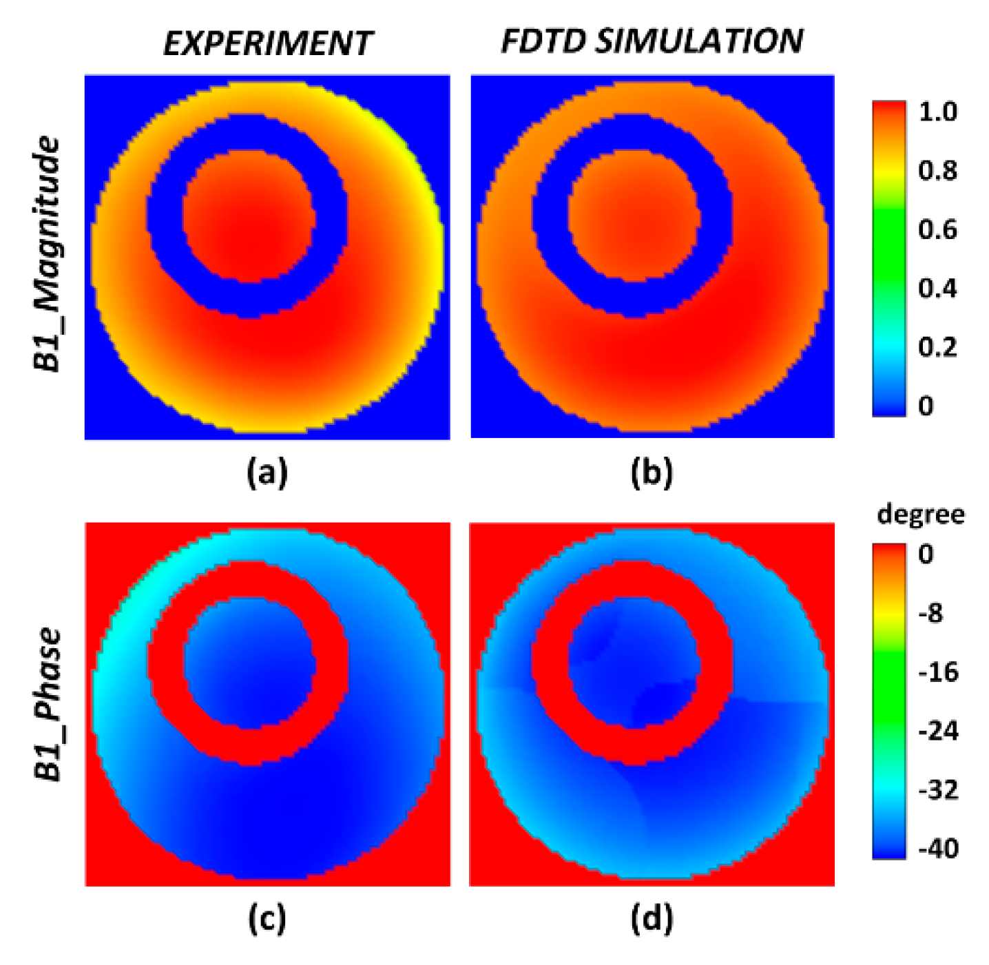
3.2. Experimental Results

The new EPT method was further verified by using experimental data obtained from the 9.4T MRI system. The measured $B_1^{+}$ field data were compared with that from the GPU-FDTD solver, as shown in Figure 6, indicating that an accurate $B_1^{+}$ field can be calculated for both the magnitude and phase. These results confirmed the accuracy of the forward solver in the new EPT approach, thus showing that stable and fast convergence can be expected. The measured $B_1^{+}$ data (including the magnitude and phase information) was firstly used to generate the EP profile by using the conventional method with the LHA.

As shown in Figure 7b,f, large reconstruction artefacts can be clearly observed in the two solutions. In the inner and outer regions of the acrylic container, more distortions are observed compared with the results from mFD and the proposed method. This is because the LHA-based method is susceptible to measurement noise; hence EP distortions still appear in those homogenous regions. Figure 7c,g showed the reconstruction results by using the mFD and Figure 7d,h are the solutions of the new EPT method. It can be observed that although the artifacts were reduced when using the mFD method, and the specific EPs were still deviated from the measured values. With the proposed method, an accurate estimation of the EPs in the two solutions can be achieved. The proposed method attempted to seek the optimum EP values of the inner and outer regions by fitting the measured and calculated $B_1^{+}$ field. This process mainly considers the global $B_1^{+}$ field distribution, thereby mitigating the local measurement noise effect and significantly improving the robustness of the algorithm. Owing to this feature, accurate EP values of the inner and outer regions can be calculated.

Table 2. Reconstructed EPs of the phantom (based on simulated data).

Compartment		Probe Measurement	Reconstructed
Inner	εr	78.5	78
	σ	0.78	0.7768
Outer	εr	78.5	78
	σ	0.43	0.4324

shows that permittivity and conductivity values can be calculated with less than 0.6% errors, which indicated the superiority of the proposed EPT in a practical utilization. The excellent results shown in Figure 7 are obtained with the available exact acrylic boundaries derived from the acquired MR image, and the EPs in segmented regions are taken as unknown constants to reconstruct through optimization. The precise position of the acrylic pixels is also known from segmentation and excluded in the EP reconstruction.

In addition to EP reconstruction, the new EPT can also provide information about the $B_z$ field, which is usually neglected in current differential and integral-based MR-EPT methods. Figure 8 shows the exported $B_z$ components from the proposed solution procedure. As expected, in the central plane of the birdcage coil, the $\left|B_z\right|$ was quite small. Close to the coil ends, the $\left|B_z\right|$ value was elevated. The availability of these magnetic field components should be helpful to improve the EPT solution and its applications in MRI.

4. Discussion

4.1. Advantages of the Proposed Method

It has been well recognized that most EPT methods developed so far are based on the second-order differential wave equation. These methods are theoretically sound but practically un-robust in real imaging applications. In particular, these methods all rely on the accurate phase information of the $B_1^{+}$ data, which is particularly challenging to obtain in ultra-high field MRI. To find EPT solutions, assumptions and simplifications have to be made and cause system errors. By directly solving Maxwell’s equations related to EPT (in which first-order differential operation only is involved) and probing dielectric properties via analysis of the $\left|B_1^{+}\right|$ data, the proposed method inversely finds solutions [38,39] with improved robustness and practicability for ultra-high field applications. This has been demonstrated in both simulation studies and phantom-based experimental testing at 9.4T. Results indicated that the proposed EPT offers a significant enhancement in the reconstruction quality compared with existing EPT approaches. Specifically, lower tissue boundary artefacts and less sensitive to measurement noise are observed, and acceptable EP reconstruction can be achieved with less than a 0.2 RMSE value when the SNR level reached 15 dB.

As shown in the experimental results, the proposed method can provide EPT solutions, as well as export full components of the magnetic and electrical fields. With the available $B_z$ profiles, one can see that near the birdcage center, the EPT reconstruction should be quite accurate without using the $B_z$ information. However, in the regions close to the birdcage end rings, neglecting the $B_z$ component would introduce system errors as the intensity of $B_z$ component becomes comparable with that of $B_x$ and $B_y$. This $B_z$ issue will be more prominent in array coil systems because of the larger value of $\left|B_z\right|/\left|B_{x,y}\right|$ in such cases, and it is therefore expected that the new EPT method can provide much better solutions when surface coils are used. Furthermore, the proposed EPT method can also export the electric fields, which cannot be measured inside patients. The availability of these field components will be particularly useful to the estimation of patient-specific SAR and also new development of imaging methods in ultra-high field MRI.

4.2. Limitations of the Proposed Method

Two main limitations can be identified regarding the proposed method. Firstly, the imaged subject needs to be modelled in the EM field solver. As it is challenging to find solutions to the formed optimization problem with millions of unknowns, the following assumption was made: one type of tissue has uniform EP values. In electromagnetic computing, a segmented MR image is required as prior information to help assign initial EP values of corresponding FDTD cells representing the imaged subject. The structure of the imaged subject can be constructed by using image registration techniques or implementing segmentation of the obtained MR images [40,41]. During optimization, several or tens of unknown variables are only required to update. With a significant dimension reduction, superior convergence can thus be achieved. Owing to an ideal experimental setup involving birdcage coil and sample phantom, the FDTD model can match the experiment shown in this work. Compared with conventional EPT approaches with z-field independency and LHA, the full-wave EM calculation is capable of regularizing the EPT solution closer to measurements. Even with the $\left|B_1^{+}\right|$ data only, the strong coupling mechanism of E- and H-fields in Maxwell’s curl equation can still faithfully find the EP values. Lastly, the proposed EP solution is sensitive to the initial setup of the EP values. We expect that the accuracy of the proposed method for human tissue mapping could be much lower than the given simple phantom and simulation results, and further validation is thus required. On the other hand, the coil structure can be obtained using a reference-based approach [42,43]. That is, using a phantom with pre-known dielectric properties, one can determine the coil information. The coil model can then be used for EPT studies. Secondly, Maxwell’s curl equations are solved by the FDTD technique, which is usually time-consuming, and may take up to several hours to converge. In this study, to balance the spatial resolution and computational cost, an mm-level grid size for the FDTD solver was found to be effective to resolve the MRI-EPT problem. In this work, we have successfully employed GPU acceleration to enable an efficient implementation of the FDTD computing (in only tens of seconds). Through appropriately applying these techniques, it is then feasible to use a standard optimization technique to retrieve accurate EP distributions in practice.

5. Conclusions

In conclusion, this work proposed a novel EPT method that reconstructs tissue dielectric properties by directly solving Maxwell’s curl equations. This method has several advantages over existing methods: (a) Without the use of second-order differential operations, the EPT solutions are more robust against $B_1^{+}$ measurement errors and noise, (b) the GPU-enabled FDTD solver allows for the efficient implementation of an iterative optimization procedure for finding the EPT solutions, and the proposed method could therefore be used in clinical environments, and (c) since $B_1^{+}$ phase information is not required in the solution procedure, the proposed method is more straightforward than many of the existing methods, particularly for the cases involving coil arrays in high-field MRI. These advantages have been validated through simulation and phantom-based experimental studies. The feasibility and effectiveness of the proposed EPT method will be further tested in human imaging at 7T, using both a birdcage coil and phased array coils.

References

1. Collins, C.M.; Liu, W.Z.; Wang, J.H.; Gruetter, R.; Vaughan, J.T.; Ugurbil, K.; Smith, M.B. Temperature and SAR calculations for a human head within volume and surface coils at 64 and 300 MHz. J. Magn. Reson. Imaging 2004, 19, 650–656. [Google Scholar] [CrossRef]
2. Aberg, P.; Nicander, I.; Hansson, J.; Geladi, P.; Holmgren, U.; Ollmar, S. Skin cancer identification using multifrequency electrical impedance-a potential screening tool. IEEE Trans. Biomed. Eng. 2004, 51, 2097–2102. [Google Scholar] [CrossRef]
3. Halter, R.; Schned, A.; Heaney, J.; Hartov, A.; Schutz, S. and Paulsen, K. Electrical impedance spectroscopy of benign and malignant prostatic tissues. J. Urol. 2008, 179, 1580–1586. [Google Scholar] [CrossRef] [PubMed]
4. Balidemaj, E.; Kok, H.; Schooneveldt, G.; Van Lier, A.; Remis, R.; Stalpers, L.; Westerveld, H.; Nederveen, A.; van den Berg, C.; Crezee, J. Hyperthermia treatment planning for cervical cancer patients based on electrical conductivity tissue properties acquired in vivo with EPT at 3T MRI. Int. J. Hyperther. 2016, 32, 558–568. [Google Scholar] [CrossRef] [PubMed] [Green Version]
5. Haacke, E.; Petropoulos, L.; Nilges, E.; Wu, D. Extraction of conductivity and permittivity using magnetic resonance imaging. Phys. Med. Biol. 1991, 36, 723–734. [Google Scholar] [CrossRef]
6. Wen, H. Noninvasive quantitative mapping of conductivity and dielectric distributions using RF wave propagation effects in high-field MRI. In Proceedings of the Medical Imaging 2003 Conference, San Diego, CA, USA, 17–20 February 2003; pp. 471–477. [Google Scholar]
7. Katscher, U.; Voigt, T.; Findeklee, C.; Vernickel, P.; Nehrke, K.; Dossel, O. Determination of electric conductivity and local SAR via B1 mapping. IEEE Trans. Med. Imaging 2009, 28, 1365–1374. [Google Scholar] [CrossRef] [PubMed]
8. Voigt, T.; Katscher, U.; Doessel, O. Quantitative conductivity and permittivity imaging of the human brain using electric properties tomography. Magn. Reson. Med. 2011, 66, 456–466. [Google Scholar] [CrossRef] [PubMed]
9. Seo, J.; Kim, M.; Lee, J.; Choi, N.; Woo, E.; Kim, H.; Kwon, O.; Kim, D. Error analysis of nonconstant admittivity for MR-based electric property imaging. IEEE Trans. Med. Imaging 2012, 31, 430–437. [Google Scholar] [PubMed]
10. Katscher, U.; Kim, D.; Seo, J. Recent progress and future challenges in MR electric properties tomography. Comput. Math. Methods Med. 2013, 2013, 1–11. [Google Scholar] [CrossRef] [Green Version]
11. Borsic, A.; Perreard, I.; Mahara, A.; Halter, R. An inverse problems approach to MR-EPT image reconstruction. IEEE Trans. Med. Imaging 2016, 35, 244–256. [Google Scholar] [CrossRef]
12. Ropella, K.; Noll, D. A regularized, model-based approach to phase-based conductivity mapping using MRI. Magn. Reson. Med. 2016, 78, 2011–2021. [Google Scholar] [CrossRef] [PubMed] [Green Version]
13. Zhang, X.; Van de Moortele, P.; Schmitter, S.; He, B. Complex B1 mapping and electrical properties imaging of the human brain using a 16-channel transceiver coil at 7T. Magn. Reson. Med. 2013, 69, 1285–1296. [Google Scholar] [CrossRef] [PubMed] [Green Version]
14. Shin, J.; Kim, M.; Cho, S.; Kim, D. Fast spin echo imaging based electric property tomography with k-space weighting via T2 relaxation (rEPT). IEEE Trans. Med. Imaging 2017, 36, 1615–1625. [Google Scholar] [CrossRef] [PubMed]
15. Lee, S.; Bulumulla, S.; Hancu, I. Theoretical investigation of random noise-limited signal-to-noise ratio in MR-based electrical properties tomography. IEEE Trans. Med. Imaging 2015, 34, 2220–2232. [Google Scholar] [CrossRef] [Green Version]
16. Liu, J.; Shao, Q.; Wang, Y.; Adriany, G.; Bischof, J.; Van de Moortele, P.; He, B. In vivo imaging of electrical properties of an animal tumor model with an 8-channel transceiver array at 7T using electrical properties tomography. Magn. Reson. Med. 2017, 78, 2157–2169. [Google Scholar] [CrossRef]
17. Liu, J.; Zhang, X.; Schmitter, S.; Moortele, P.; He, B. Gradient-based electrical properties tomography (gEPT): A robust method for mapping electrical properties of biological tissues in vivo using magnetic resonance imaging. Magn. Reson. Med. 2015, 74, 634–646. [Google Scholar] [CrossRef] [Green Version]
18. Liu, C.; Jin, J.; Guo, L.; Li, M.; Tesiram, Y.; Chen, H.; Liu, F.; Xin, X.; Crozier, S. MR-based electrical property tomography using a modified finite difference scheme. Phys. Med. Biol. 2018, 63, 14. [Google Scholar] [CrossRef]
19. Gurler, N.; Ider, Y. Gradient-based electrical conductivity imaging using MR phase. Magn. Reson. Med. 2016, 77, 137–150. [Google Scholar] [CrossRef]
20. Hafalir, F.; Oran, O.; Gurler, N.; Ider, Y. Convection-reaction equation based magnetic resonance electrical properties tomography. IEEE Trans. Med. Imaging 2014, 33, 777–793. [Google Scholar] [CrossRef] [Green Version]
21. Wang, Y.; Van de Moorele, P.; He, B. Contrast conformed electrical properties tomography (CONCEPT) based on multi-channel transmission and alternating direction method of multipliers. IEEE Trans. Med. Imaging 2018, 99, 349–359. [Google Scholar] [CrossRef]
22. Schmidt, R.; Webb, A. A new approach for electrical properties estimation using a global integral equation and improvements using high permittivity materials. J. Magn. Reson. 2016, 262, 8–14. [Google Scholar] [CrossRef] [PubMed]
23. Leijsen, R.; Brink, W.; van den Berg, C.; Webb, A.; Remis, R. 3-D contrast source inversion-electrical properties tomography. IEEE Trans. Med. Imaging 2018, 37, 2080–2089. [Google Scholar] [CrossRef] [PubMed]
24. Guo, L.; Jin, J.; Liu, C.; Liu, F.; Crozier, S. An efficient integral-based method for three-dimensional MR-EPT and the calculation of the RF-coil induced Bz field. IEEE Trans. Biomed. Eng. 2018, 65, 282–293. [Google Scholar] [CrossRef] [PubMed]
25. Guo, L.; Jin, J.; Li, M.; Wang, Y.; Liu, C.; Liu, F.; Crozier, S. Reference-based integral MR-EPT: Simulation and experiment studies on the 9.4T MRI. IEEE Trans. Biomed. Eng. 2019, 66, 1832–1843. [Google Scholar] [CrossRef]
26. Hong, R.; Li, S.; Zhang, J.; Zhang, Y.; Liu, N.; Yu, Z.; Liu, Q. 3-D MRI-Based Electrical Properties Tomography Using the Volume Integral Equation Method. IEEE Trans. Microw. Theory Tech. 2017, 65, 4802–4811. [Google Scholar] [CrossRef]
27. Abenius, E.; Strand, B. Solving inverse electromagnetic problems using FDTD and gradient-based minimization. Int. J. Numer. Meth. Eng. 2006, 68, 650–673. [Google Scholar] [CrossRef]
28. Takenaka, T.; Tanaka, T.; Harada, H.; He, S. FDTD approach to time-domain inverse scattering problem for stratified lossy media. Microw. Opt. Techn. Let. 1997, 16, 292–296. [Google Scholar] [CrossRef]
29. Chi, J.; Liu, F.; Weber, E.; Li, Y.; Crozier, S. GPU-accelerated FDTD modeling of radio-frequency field-tissue interactions in high-field MRI. IEEE Trans. Biomed. Eng. 2011, 58, 1789–1796. [Google Scholar]
30. Taflove, A.; Hagness, S. Computational Electrodynamics: The Finite-Difference Time-Domain Method, 3rd ed.; Artech House: Boston, MA, USA, 2005. [Google Scholar]
31. Hoult, D. The principle of reciprocity in signal strength calculations—A mathematical guide. Concepts Magn. Reson. 2000, 12, 173–187. [Google Scholar] [CrossRef]
32. Andreas, C.; Wolfgang, K.; Eckhart, G.; Katharina, H.; Marcel, Z.; Esra, N.; Rascher, W.; Janka, R.; Bautz, W.; Chen, J. The virtual family-development of surface-based anatomical models of two adults and two children for dosimetric simulations. Phys. Med. Biology. 2010, 55, 23–38. [Google Scholar]
33. Joines, W.; Dhenxing, Y.; Jirtle, R. The measured electrical properties of normal and malignant human tissues from 50 to 900 MHz. Med. Phys. 1994, 21, 547–550. [Google Scholar] [CrossRef] [PubMed]
34. Dietrich, O.; Raya, J.G.; Reeder, S.B.; Reiser, M.F.; Schoenberg, S.O. Measurement of signal-to-noise ratios in MR images: Influence of multi-channel coils, parallel imaging, and reconstruction filters. J. Magn. Reson. Imaging. 2007, 26, 375–385. [Google Scholar] [CrossRef] [PubMed]
35. Akoka, S.; Franconi, F.; Seguin, F.; Pape, A. Radiofrequency map of an NMR coil by imaging. Magn. Reson. Med. 1993, 11, 437–441. [Google Scholar] [CrossRef]
36. Cunningham, C.; Pauly, J.; Nayak, K. Saturated double-angle method for rapid B 1 + mapping. Magn. Reson. Med. 2006, 55, 1326–1333. [Google Scholar] [CrossRef]
37. Lier, A.; Brunner, D.; Pruessmann, K.; Klomp, D.; Luijten, P.; Lagendijk, J.; van den Berg, C. B1+ phase mapping at 7T and its application for in vivo electrical conductivity mapping. Magn. Reson. Med. 2012, 67, 552–561. [Google Scholar] [CrossRef]
38. Ider, Y.; Boga, C. Inverse problem approach to cr-MREPT. In Proceedings of the ISMRM 27th Annual Meeting & Exhibition, Montreal, QC, Canada, 11–16 May 2019. abstract number 5052. [Google Scholar]
39. Rahimov1, A.; Litman, A.; Ferrand, G. MRI-based electric properties tomography with a quasi-Newton approach. Inv. Prob. 2017, 33, 105004. [Google Scholar] [CrossRef] [Green Version]
40. Devi, C.; Chandrasekharan, A.; Sundararaman, V.; Alex, Z. Neonatal brain MRI segmentation: A review. Comput. Biol. Medicine. 2015, 64, 163–178. [Google Scholar] [CrossRef]
41. Despotovic, I.; Goossens, B.; Philips, W. MRI segmentation of the human brain: Challenges, methods, and applications. Comput. Math. Methods Med. 2015, 2015, 1–23. [Google Scholar] [CrossRef] [Green Version]
42. Liu, F.; Beck, B.; Xu, B.; Fitzsimmons, J.; Blackband, S.; Crozier, S. Numerical modelling of 11.1 T MRI of a human head using a MoM/FDTD method. Concepts Magn. Reson. Part B Magn. Reson. Eng. 2005, 24, 28–38. [Google Scholar] [CrossRef]
43. Jin, J.; Liu, F.; Weber, E.; Crozier, S. Improving SAR estimations in MRI using subject-specific models. Phys. Biol. Med. 2012, 57, 8153–8171. [Google Scholar] [CrossRef]
Figure 1. Frameworks of different types of Electrical Properties Tomography (EPT) methods, (a) the local homogeneity assumption (LHA)-based solution [7,8], (b) the second-order differential wave equation-based solution [16,17,18,19,20], (c) integral equation-based solution [11,23,24,25,26], and (d) the proposed EPT approach. It is noted that the proposed method finds the EPT solution without accessing the phase information of the radiofrequency (RF) field.
Applsci 10 03318 g001
Figure 2. The finite-difference-time-domain (FDTD) configuration. Here, a 12-leg birdcage coil was modelled and loaded with a subject (phantom or head); a perfect electric conductor (PEC) was placed around the birdcage coil to simulate the RF shield, and perfectly matched layers (PML) boundary conditions were placed at the top and bottom of the computation domain. With the graphics processing unit (GPU) computing, the FDTD calculation of the electromagnetic (EM) fields only took about 18 s for the given case involving 1.4 million Yee-cells.
Applsci 10 03318 g002
Figure 3. (a) The photo of the phantom used in the experiment and (b) the MR image obtained at 9.4 Tesla (T).
Applsci 10 03318 g003
Figure 4. The target and reconstructed EP profiles under different SNR levels (15~35 dB). (a,e) are the target EPs. (b,f) are the results under SNR level is 15 dB. (c,g) are the results under SNR level is 25 dB. (d,h) are the results under SNR level is 35 dB.
Applsci 10 03318 g004
Figure 5. The root-mean-square-errors (RMSE) concerning the reconstructed εr and σ by using the traditional LHA-based method (blue line), the recently proposed modified Finite-Difference (mFD) method (purple line) and the proposed method (red line) under different SNR levels (from 55 dB to 15 dB). (a,d) retrieve EP’s values in the cerebrospinal fluid (CSF) CSF region, (b,e) retrieve EP’s values in the white matter’s region, (c,f) the retrieved EP’s values in the gray matter’s region.
Applsci 10 03318 g005
Figure 6. (a,c) indicate the magnitude and phase of the measured B 1 + data. (b,d) indicate the magnitude and phase of the calculated B 1 + data from the GPU-FDTD solver.
Applsci 10 03318 g006
Figure 7. (ad) indicate the measured permittivity and the reconstructed one by using the traditional method based on LHA (Helmholtz), the wave-equation-based finite-difference method (modified Finite-Difference (mFD)) and the proposed method, respectively. (eh) indicate the measured conductivity and the reconstructed one by using the three methods, respectively.
Applsci 10 03318 g007
Figure 8. The calculated magnitude and phase of the Bz field component from the experiment, (a,d): on the upper plane, which is 0.85 mm away from the central slice, (b,e): on the central slice, (c,f): on the lower plane, which is 0.85 mm away from the central slice.
Applsci 10 03318 g008