Article

Multi-Period Maximal Covering Location Problem with Capacitated Facilities and Modules for Natural Disaster Relief Services

1
Division of Mathematical Science for Social Systems, Department of Systems Innovation, Graduate School of Engineering Science, Osaka University, Machikaneyama-Cho 1-3, Toyonaka City, Osaka 560-8531, Japan
2
Graduate School of Natural Sciences, Department of Industrial Innovation Engineering, Okayama University, Tsushima-naka 3-1-1, Kita-ku, Okayama City, Okayama 700-8530, Japan
3
Department of Industrial Engineering, Faculty of Engineering, Alzahra University, Tehran 1993893973, Iran
4
School of Strategy and Leadership, Faculty of Business and Law, Coventry University, Coventry CV1 5FB, UK
*
Authors to whom correspondence should be addressed.
Submission received: 27 October 2020 / Revised: 17 December 2020 / Accepted: 19 December 2020 / Published: 4 January 2021

Abstract

:
The paper aims to study a multi-period maximal covering location problem with the configuration of different types of facilities, as an extension of the classical maximal covering location problem (MCLP). The proposed model can have applications such as locating disaster relief facilities, hospitals, and chain supermarkets. The facilities are supposed to be comprised of various units, called the modules. The modules have different sizes and can transfer between facilities during the planning horizon according to demand variation. Both the facilities and modules are capacitated as a real-life fact. To solve the problem, two upper bounds—(LR1) and (LR2)—and Lagrangian decomposition (LD) are developed. Two lower bounds are computed from feasible solutions obtained from (LR1), (LR2), and (LD) and a novel heuristic algorithm. The results demonstrate that the LD method combined with the lower bound obtained from the developed heuristic method (LD-HLB) shows better performance and is preferred to solve both small- and large-scale problems in terms of bound tightness and efficiency especially for solving large-scale problems. The upper bounds and lower bounds generated by the solution procedures can be used as the profit approximation by the managerial executives in their decision-making process.

1. Introduction

The maximal covering location problem (MCLP), introduced by Church and Revelle [1] maximizes the demands covered by the specified number of facilities to be located. MCLP has a wide range of applications in locating public facilities—such as health care facilities, police stations, schools, and fire stations, etc.—but it can also be used in locating private sector facilities such as warehouses, distribution centers, chain supermarkets, etc. Developing a model for each of the applications with the specific real situation, resulted in various extensions developed for the covering models since their introduction. The hierarchical MCLP [2,3], probabilistic MCLP [4,5] MCLP in competitive environments [6], large-scale dynamic MCLP [7], continuous MCLP for natural disasters [8], and maximal hub location problem [9] are some examples among the vast literature of the MCLP. The growing attention and interest in covering location problems are due to their applications. However, the developed models are far from real-world problems and there is still much work to do [10]. Farahani et al. [11] suggested the areas that could be considered for further research, such as having different facilities and capacitated facilities. In the current paper by considering modular capacitated facilities, we attempt to modify a closer model to real-world problems such as disaster relief service location problems.
Disaster relief services have been receiving global attention due to the scarcity of resources, accountability concerns, and the potential opportunities provided by advances in global information technologies [12]. One of the solutions to overcome the scarcity of resources is modularization. Modularization of services in the case of disaster can be interpreted as what the World Vision International is doing, i.e., relief supplies are stored in four locations globally, and can be immediately shipped anywhere in the world [13]. Furthermore, using mobile housing structures—such as temporary and portable offices, shelters, restrooms, warehouses, etc.—even modularization of the facilities is possible. These mobile structures are commonly used now and result in fast construction that is profoundly essential in a disaster situation like the Chinese government action caused by COVID-19 in building the Wuhan city 1000 bed hospital in 10 days utilizing the prefabricated constructions [14]. In modular facilities, the mobile structures can move to the other areas when their mission is finished and it can result in total cost reduction because of the reusability of modules in other situations like the unique solution Japan has decided to offer praying rooms during the 2020 Olympic games [15]. Attempting to optimize the module assignment decision, it increases flexibility [16], reduces the costs and as a result increases sustainability. The rescue missions [17], temporary housing [18], and goods distribution [19] in a disaster situation are more or less investigated in the literature, but addressing the service providing facilities in a modular and dynamic framework remains as a research gap that this gap is fulfilled in the current study.
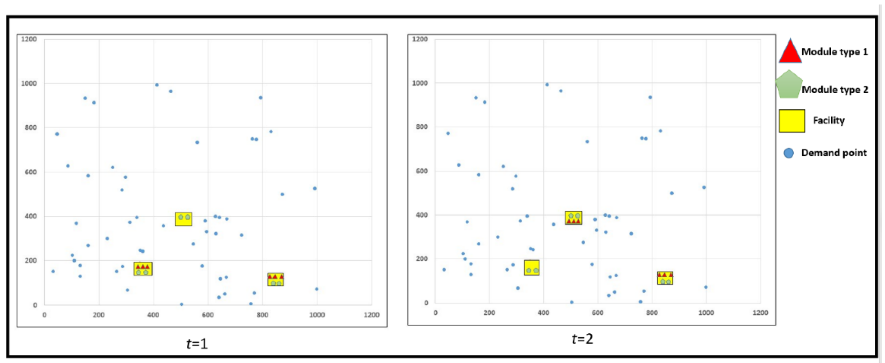
In this paper, another extension of the MCLP is presented that mainly concentrates on the structure of the facilities to be located. Almost all facilities are composed of different units and departments, which provide a special kind of services or products called modules of facilities. In real examples of hospital application, facilities are hospital location and modules are ambulances, operating rooms and staff members over time horizon. In the disaster relief centers, facility is the location of centers and the modules are tents, waters, foods, etc. In the supermarkets, facility is the location of supermarkets and the modules are hot food shelf, beverage shelf, cold product shelf, etc. In a practical setting, e-commerce companies adopt different pricing policies over different time periods under different demand forecasts. Those real-world problems and demand variation in different time periods necessitate to develop a multi-period model that optimizes the objective value in different time periods looking for optimal solutions for assigning the modules to the facilities and allocating the demand points to the modules. The proposed mathematical model in this paper locates the capacitated facilities at the beginning of the planning horizon and then in each time period, assigns the optimum number of capacitated modules to the facilities with the objective of maximizing the covered demands and minimizing the module assignment cost. Modularization of the facilities provides the opportunity to develop more cost and energy-efficient smart facilities. One of the main applications of this model is for a disaster relief situation in which government is the decision maker. The service request of demand points is not the same in all disasters and depends on many factors such as the severity of the disaster. Demand fluctuation can be reflected by having the multi-period planning model. In this application, the facilities are the disaster relief centers, the modules can be ambulances, trucks, helicopters, first aid units, food providing units, sleeping tents, shower rooms, etc. and the demand points are the residents or residential areas affected by the disaster and having service requests. The locations of a limited number of disaster relief facilities are first determined and having the assumption that each disaster is happening in one of the time periods of the planning horizon, the modules are assigned to the located facilities. The modules are capacitated and they have different sizes. The optimal number and size of each module’s kind that should be assigned to the relief centers are determined by the model in order to have maximized allocated and covered demand points. After terminating the mission of modules in one of the affected areas in one period, in the next period the modules can be transferred to the other affected area to provide service there.
Other applications of this model can be in locating and service providing of chain convenient stores as the facilities and decision maker is the operation planning department. There are many product categories available in these stores that can be assumed as the modules and customers are the demand points. Most of the time, there is no need to provide all kinds of products in all stores when there might be not enough demand for them in different seasons. According to our model, the predefined stores can be located using the developed model at the beginning of the planning horizon. Afterwards, according to the demand variation in different areas and time periods, the optimal number and size of modules are assigned to the located stores. The objective of maximizing the covered demands from one hand, and minimizing the cost of module assignments on the other hand creates a good balance between service quality and cost management.
The mathematical model of the multi-period modular capacitated maximal covering location problem (MMCMCLP) is a mixed integer linear programming model. The objective is to maximize the profit that is obtained from the income of covering demand points and the cost of module assignment. Accordingly, three kinds of decisions are determined by MMCMCLP as:
  • Location of the predefined number of facilities;
  • Type and number of each module assigned to the located facilities in each time period during the planning horizon;
  • Percentage of allocated demands of points to the assigned modules in each time period.
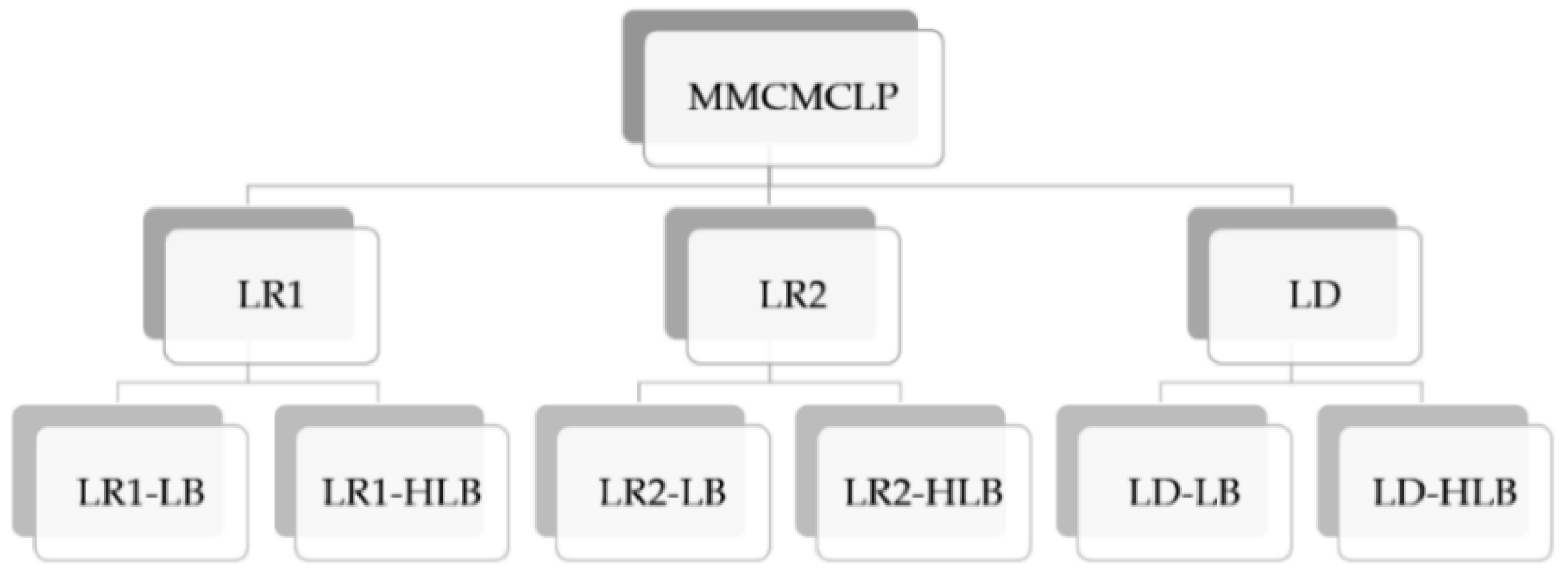
The small-size test instances can be solved to optimality using general solvers such as CPLEX. As the size of the problems increases, this solver is unable to solve the problems. To overcome this difficulty, a Lagrangian decomposition-based algorithm is developed that obtains an upper value and lower value for the optimal objective value, for which the decision makers can be assured that their profit is a value between the generated bounds and will not exceed these values. For MMCMCLP that is a maximization problem, the Lagrangian relaxation (LR) can generate an upper bound on the optimal objective value. Furthermore, many possible relaxations have been examined to figure out the relaxation of which constraints yields to the most time-efficient subproblem. In order to be able to provide sufficient evaluations on the possible methods, two procedures are proposed. In both approaches, the upper bounds are calculated by using two different sets of relaxed constraints and a decomposed problem. We also have developed two procedures to obtain a lower bound for the optimal objective value of the proposed model. In the first approach, the lower bound is computed by generating feasible solutions. In the second procedure, the lower bound is obtained from a developed heuristic method that locates the predefined number of facilities according to the criteria of more capacity and coverage of demands. Afterward, a sufficient number of modules with lower cost and more capacity would be assigned to the located facilities to maximize the number of allocated demands. Two relaxation problems and a decomposed problem provide three different upper bounds, which in addition to two lower bounds obtained from constructed feasible solutions and a heuristic method provide various bounds. The best method is the one that can produce the tightest upper and lower bounds, for which the bounds obtained from different approaches are analyzed to investigate the tightest bounds to select the best method.
The main contributions and innovations of this study are summarized as follows:
  • We propose a new model called multi-period modular capacitated maximal covering location problem, which in addition to the facility location decisions, it determines module assignment and demand allocation decisions in different periods of the planning horizon.
  • The configuration of the facilities using the modularity concept results in having three-level facilities. Different size of modules (first level) along with having a different kind of modules (second level) makes it possible to have different facilities (third level).
  • An efficient Lagrangian decomposition-based method is developed to derive the upper bound. Furthermore, two different lower bounds are developed and compared to synthesize the proposed Lagrangian decomposition (LD) method.
  • Different upper bounds and lower bounds from various approaches are compared to evaluate the efficiency and tightness of the bounds. Our findings approve the superiority of the bounds obtained from Lagrangian decomposition-based (upper bound) and heuristic method (lower bound) over large-scale instances.
  • Sensitivity analysis for the problem is conducted to investigate the validity of the proposed model under different parameters.
The remainder of the paper is organized as follows. Section 2 reviews the related studies. The mathematical model for the MMCMCLP is provided in Section 3. In Section 4, the solution approach to obtain Lagrangian upper bound integrated with a heuristic method to achieve the lower bound of the problem is proposed. Then numerical examples are analyzed in Section 5 and finally, conclusions are discussed in Section 6.

2. Literature Review

This section surveys the current literature of this study regarding the three major topics as MCLP, modular location problem, and Lagrangian relaxation method.

2.1. MCLP

In the basic formulation of the maximal covering location problem, there is no limitation for the capacity of the located facilities and they are formulated for a single time period. Uncapacitated facility means that service by each facility can be provided limitless as long as the recipients are within the coverage standard. However, in most of the real-world applications of covering problems, considering capacity limitations for facilities is a more realistic assumption. Most facilities have limits on service capabilities due to physical, political, structural, regional, and other reasons [20].
Another restrictive assumption of basic covering location problems is considering the planning through the time horizon called multi-period or dynamic models. So-called dynamic location models consider a multi-period operating context where the demand varies between different time periods [21]. In multi-period MCLP, decision makers are interested in finding the optimal way of locating a definite number of facilities in different periods. The application of multi-period MCLP can be found in locating emergency service centers in populated regions that on-road accidents may happen and the number of facilities to be located may fluctuate between different periods of time because of daily traffic, weather situation, etc. Moreover, each opened facility at the beginning of a time period can be closed at the end of that time period in a multi-period MCLP [22]. In this regard, Marin et al. [23] addressed a general discrete covering location model in which they considered a finite planning horizon that is partitioned into several time-periods. Because the time periods are not necessarily of the same length and in each period, it is allowed that multiple facilities/equipment can be opened or closed in each location at some cost. Furthermore, Marin et al. [23] assumed that each demand point should be covered by at least a specific number of facilities and coverage lower than the minimum threshold undergoes a time-dependent penalty cost. These features of the studied problem result in a different way of demand point allocations to the facilities in each time period.
Bagherinejad and Shoeib [24] studied a multi-period maximal covering location problem in which the total number of facilities that have to be opened, is located gradually over time. From this perspective, their model is an implicitly dynamic model. Another characteristic of their developed model is the dynamic capacity for each of the located facilities. As the application of their model is locating ambulances in emergency bases, locating a different number of ambulances in each time period makes it possible to set different levels of capacities in each time period. Vatsa and Jayaswal [25] developed the multi-period capacitated maximal covering problem considering uncertainties in server availability. Their problem addressed allocating doctors to non-operational primary health centers and as the population that needs to be served by the facilities was changing over time, they studied their problem in different time periods.

2.2. Modular Location Problem

Modularity is a strategy recognized by academia and the industry and plays an important role in the development of sustainable systems [26]. Modularity is also one of the newest concepts in location problems. One can classify the models which use the concept of modularity in two categories:
(1) Modularity which happens in points. For instance, Correia and Melo [27] presented a multi-period facility location problem with modular capacity adjustments and flexible demand fulfillment. In their model, customers were divided according to their sensitivity to delivery lead times. They also proposed two mixed integer linear programming formulations and provided an extensive numerical study on randomly generated data with different demand patterns. More recently, Allman and Zhang [28] addressed a modular facility location problem with application in the chemical industry in a way that modules assignment should be conducted considering the fact that one module product is necessary for the operation of the next module. In addition to this consideration, Allman and Zhang’s model is capable of assigning modules with different capacities. Silva et al. [29] studied a dynamic facility location problem with modular capacities as an extension of well-known location-allocation problem with capacity expansions possibilities that can be performed via a finite set of projects, and modules are represented as capacity blocks in facilities. As the problem is studied in a finite time horizon of discrete periods and module relocation costs are not considered, the modules can easily close in one facility and open in other one in each time period to optimize the objective demand points allocations.
(2) Modularity that happens in arcs. Tanash et al. [30] presented two mixed integer programming formulations, a flow-based and a path-based formulation for the modular hub location problem. Their problem formulated the flow-dependent transportation costs using modular arc costs and then they compared the models using linear programming relaxation bounds. Mikić et al. [31] addressed a capacitated modular single assignment hub location problem having modular link capacities between nodes and hubs. They also solved the proposed model with an extension of existing neighborhood structures called a general variable neighborhood search. In a similar attempt, Fard and Alfandari [32] investigated the trade-offs between the stepwise cost function and its linear approximation for the modular hub location problem. The modularity in their work arose from the transportation costs depicted as a stepwise function of the number of vehicles that had a significant cost reduction, which could not be properly measured by using a simple linear cost function.
According to the models described above, the MMCMCLP considers the modularity that happens in the arcs. There has not been any problem that focuses exclusively on modularity in maximal covering location problem. In addition, MMCMCLP is considered in a dynamic environment and capacitated facilities are located while their corresponding modules with suitable sizes are assigned to the facilities in each period.

2.3. Lagrangian Relaxation

During the last decade, various publications appeared using heuristics and meta-heuristics to solve the MCLP. Lagrangian relaxation (LR) is one of these heuristics which has been used by many researchers to find bounds for different problems. For example, Correia and Captivo [33] developed a Lagrangian heuristic for their modular capacitated location problem. There have been many other papers that used the LR-based algorithms to solve their models. Table 1 reviews the most important models in the area. There are various trends in using Lagrangian heuristics: applying LR just for producing lower bound, proposing heuristics for computing of both lower and upper bounds, using a fixed upper bound and try to propose lower bound heuristic and decomposing the main problem into sub-problems and then applying the mentioned procedures. Table 1 shows the most important papers related to the procedure used in this paper. From Table 1, it can be concluded that most researchers have proposed heuristics for both lower and upper bounds.
Fathollahi-Fard et al. [34] has used an adaptive LR method to solve the problem of water supply and wastewater collection network design as a minimization problem to address the drought problem of Urmia lake in Iran. The adaptive LR solves the relaxed problem and its solution is accepted as the lower bound. Afterward, to obtain the feasible solution as the upper bound the solutions for continuous variables of the relaxed problem are fixed and used as parameters and the binary variables are modified in a way that the feasibility of the solution is approved. The Lagrangian multiplier is then updated and the procedure is repeated until the last defined iteration. Similarly, Hamdan and Diabat [35] used LR method to solve the multi-objective model for a stochastic blood supply chain that was reformulated as a single objective and robust model before utilizing LR. The LR method developed by Hamdan and Diabat [35] relaxed one of the constraints and the solution for this relaxed problem was set as the lower bound. To convert the infeasible solutions to feasible solutions and obtain the upper bound they used a heuristic method. In addition, Zhang et al. [36] developed a Lagrangian-based decomposition algorithm for train rescheduling and track emergency maintenance problem that happens under a rolling horizon framework. To overcome the difficulty of solving the complex model, they decomposed the original problem in two sub-problems and computed the LR for each problem in a parallel procedure. As their proposed model is a collaborative real-time optimization model, the developed Lagrangian-based decomposition method could reduce the computation effort for the real-time implementation, and realized online feedback correction. Nishi et al. [37,38] addressed the LR with cut for hybrid flowshop scheduling problems and the LR with Petri nets for routing problems for AGVs.

3. Problem Definition

3.1. Multi-Period Modular Capacitated Maximal Covering Location Problem (MMCMCLP)

Suppose we are going to locate some facilities (like hospitals or disaster relief centers) in a city. Because of capital limitation, only a limited number of p facilities are going to be established that aim to cover the maximum number of demands. After defining the location of the facilities, according to the demand requests at each time period from each module, the assignment of modules and their proper size would be determined to maximize the total coverage amount minus the cost of establishing modules.
The modules of the facility have four main properties:
  • Each module comes in different sizes. It can be chosen from different sizes to increase the service quality offered to demand points to overcome the service shortages or having idle units.
  • The modules are portable and they can be transferred among the facilities when there is more request in another facility. The transferability is an important specification of modularity design that yields to flexibility in the system and reduces costs. The portability of most modules helps to provide a good level of service to demand points without having to provide more modules.
  • As there are no constraints on the number of modules to be assigned to facilities, more of them can be established in the coming periods (if there is increasing demand) as expansion plans to have more coverage of demand points. The number and the location of the facilities after the decisions are made would be fixed for all time periods, but there is no such limitation for modules.
  • Each size of the modules has a known lower and upper-level service capacity for which, the total number of allocated points should be between this lower and upper level capacity. On the other hand, the total number of demands allocated to all kinds of modules cannot exceed each facility’s capacity.

3.2. Mathematical Formulation

In the developed model, it is assumed that the coverage of points obeys the gradual coverage rule in which by increasing the distance from full coverage radius   ( S ) the coverage value reduces using a partial coverage function as f ( d i j )   that 0 < f ( d i j ) < 1 . The proposed MMCMCLP can be formulated as a mixed integer linear programming (MILP) problem in the following way.
Consider the following indices, parameters and decision variables:
Sets and Parameters:
i I The index and set of potential facilities.
j J The index and set of demand points.
l L The index and set of modules.
k l K l The index and set of size indices for module l   ( l L ) .
t T The index and set of time periods.
S The maximum full coverage distance.
S The maximum partial coverage distance   ( S > S ) .
d i j Distance, traveling time or cost between facility i   and demand point j .
g i j The level of coverage provided by the facility i to the demand point j .
g i j = {   1 i f   d i j S   f ( d i j ) i f   S < d i j S   0 S   < d i j
f ( d i j )   Partial coverage function, where 0 < f ( d i j ) < 1 .
a j l t The demand of point j   from the service of module l in period t .
b l k l The lower level of capacity for module l   with the size indices of k l .
B l k l The upper level of capacity for module l   with the size indices of k l .
α j The profit gained by coverage of demand point j .
β i The capacity of facility i .
h i l k l t The cost of establishing module l with size indices k l at facility i at period t .
p The number of facilities to be located.
Decision variables:
v i   Binary variable which equals 1 if a facility is located at point   i .
y i l k l t Binary variable which equals 1 if module l with size indices of k l is sited at facility i at period t .
x i j l t Coverage amount of demand point j   from module l   of facility i at period t .
Then, the proposed model is as follows:
( MMCMCLP ) Max   i I j J l L t T   α j g i j a j l t x i j l t i I l L k l K l t T h i l k l t y i l k l t    
k l K l y i l k l t v i   i , l , t
i I x i j l t 1   j , l , t
j J a j l t x i j l t k l K l b l k l y i l k l t   i , l , t
j J a j l t x i j l t k l K l B l k l y i l k l t   i , l , t
l L j J a j l t x i j l t β i v i   i , t
i I v i p
y i l k l t { 0 ,   1 } , v i { 0 ,   1 } , x i j l t 0   i , j , l , k l , t
The objective function (1) seeks to maximize the profit gained from the covered allocated demands while simultaneously minimizing the total cost of assigning the modules. It should be noted that the parameter α j is used to avoid having a bi-objective function structure. Constraints (2) ensure that if there not exists an established facility at site   i , no module is allowed to be sited there and only one size of each module can be sited in a facility. Constraints (3) imply that the total coverage of each demand point from all the facilities can be at most 1. Constraints (4) and (5) imply both, that if the module of size k l   is opened at facility i , the maximum and minimum capacity of that module cannot be exceeded. These constraints are also the allocation constraints for demand points that state the coverage of a point x i j l t is forbidden unless there is any size of module l sited at facility i in period   t . Constraint (6) implies that all demands allocated to modules in an opened facility i should not exceed its capacity. Constraint (7) ensures that the total number of located facilities should be at most   p . Constraint (8) imposes the ranges of decision variables.
As the MCLP is NP-hard [45], MMCMCLP would also belong to the category of NP-hard problems. Therefore, it is not possible to find a solution in a reasonable time for large dimensions of the problem for which in the next section, the solution procedures are indicated to solve real-world size problems.

4. Solution Procedure

There are three methods namely exhaustive enumeration, mathematical programming, and heuristic approaches to solve the location problems. Heuristic approaches can solve large size problems, but do not guarantee to reach an optimal solution [46]. Lagrangian relaxation-based heuristics have also been applied to many combinatorial optimization problems [47]. The quality of the solution is controlled by the upper and lower bounds provided by the LR procedure. Geoffrion and Bride [48] as one of the pioneers in studying LR to solve facility location problems, obtained theoretic and geometric insights relating the value of an LR to the usual linear programming relaxation (LPR). Their results show that LR yields a great improvement over LPR at only a small additional computational cost and cutting-planes far superior to Gomory fractional cuts. They also suggested a similar in-depth analysis of LR applied to other important classes of problems as the one is performed in this paper.
Pirkul and Schilling [49] have studied the capacitated MCLP in which the facilities can provide either a primal service for demand points or back-up service. To solve their integer linear programming model, they applied the LR method by relaxing the demand (primary and back-up) allocation constraints and proposed a heuristic method to construct a feasible solution from the subgradient method.
In this section, different possible relaxations for MMCMCLP and solving procedure for each possible relaxation are presented. In addition, a heuristic algorithm, to obtain the lower bound, is presented in the last subsection. For each proposed relaxed problem, two approaches will be used to solve it. In the first approach, the lower bound can be obtained and updated in iterations using feasible solutions and in the second approach, the lower bound would be obtained from the heuristic method.

4.1. Upper Bounds

4.1.1. LR1

There are several Lagrangian relaxations for MMCMCLP. By using this procedure, a hard problem is converted into a relatively easy one by relaxing sets of complicated constraints. After testing possible combinations of constraints to be relaxed, in the first relaxation problem (LR1) the set of constraints (3)–(5) have been chosen to be relaxed. Let μ j l t 0     j , l , t ,   λ i l t   0     i , l , t ,   γ i l t   0   i , l , t , be the multipliers associated with constraint set (3)–(5), respectively. Then, the Lagrangian problem LR1 is defined as:
(LR1)
Z L R 1 =   Max   i I j J l L t T   α j g i j a j l t x i j l t i I l L k l K l t T h i l k l t y i l k l t     + i I j J l L t T   μ j l t   ( 1 x i j l t ) + i I l L t T λ i l t ( j J a j l t   x i j l t k l K l b l k y i l k l t   )   +   i I l L t T γ i l t ( k l K l B l k y i l k l t   j J a j l t   x i j l t )
Subject to (2), (6)–(8).
The objective function of the problem LR1,   Z L R 1 , provides an upper bound on the objective function of the MMCMCLP for μ j l t 0   j , l , t ,   λ i l t   0   i , l , t ,   γ i l t   0   i , l , t .

4.1.2. LR2

Another possible combination of constraints to be relaxed is the set of constraints (3) and (6). Let ζ j l t 0   j , l , t and   χ i t   0     i , t be the multipliers associated with constraint set (3) and (6), respectively. Then the Lagrangian relaxation problem, LR2 is defined as:
(LR2)
Z L R 2 =   Max   i I j J l L t T   α j g i j a j l t x i j l t i I l L k l K l t T h i l k l t y i l k l t     + j J l L t T ζ j l t   ( 1 i I x i j l t ) + i I t T χ i t ( β i v i j J l L a j l t   x i j l t )
Subject to (2), (4), (5), (7), and (8).
The objective function of the problem LR2, Z L R 2 , provides an upper bound on the objective function of the MMCMCLP for ζ j l t 0   j , l , t ,   and   χ i t 0   i , t .

4.1.3. Lagrangian Decomposition (LD)

When the Lagrangian multipliers ζ j l t and χ i t   are fixed, the relaxed model can be decomposed into two subproblems. The first (SubP1) determines the facility locations. After solving this problem, the set of locations would be categorized as I o I that refers to the located and opened facilities and I N o I that would be the set of locations that there is not opened facilities in them and we have I = I o   I N o and I o   I N o = . For I o I the second subproblem is defined as (SubP2) that assigns modules to each opened facility and allocates the demand points to the modules. SubP1 and Subp2 are as follows:
( SubP 1 ) Z L D 1 =   Max   i I t T χ i t β i v i
Subject to (7) and (8).
( SubP 2 ) Z L D 2 =   Max   i I o l L t T ( j J   ( α j g i j a j l t ζ j l t χ i t a j l t   )   x i j l t k l K l h i l k l t y i l k l t   ) + j J l L t T ζ j l t  
Subject to (2), (4), (5), and (8).
As the constraints (3) are relaxed there is no restricting constraint for the amount of coverage for demand points and they can have any positive value. The valid inequality (13) is added to SubP2 (as well as to LR1 and LR2), which is a redundant constraint for the primal MMCMCLP. The SubP2 is solved with the addition of (13) to obtain results for variables y i l k l t and x i j l t . An interesting feature of the SubP2 is that this problem can be decomposed and solved for each i I o , l , t .
x i j l t k l K l y i l k l t   i I o , j , l , t  
We use the subgradient method to compute   Z L D = Z L D 1 + Z L D 2 .

4.2. Lower Bounds

We develop two lower bound procedures for MMCMCLP. The first one uses the solutions obtained from LR1, LR2, and LD and constructs a feasible solution as the lower bound. The second lower bound procedure is a novel heuristic method.

4.2.1. Lower Bound from Feasible Solutions

Z L B is the lower bound to the MMCMCLP that can be calculated by fixing the variables v i τ and y i l k l t τ in constraints (3)–(6) and calculating the objective function (1) at the τ th iteration and solving the problem by a branch and bound (B&B) procedure using a general-purpose solver.

4.2.2. Lower Bound Heuristic on MMCMCLP

In this section, a heuristic method to obtain the lower bound for the MMCMCLP is presented. This heuristic method produces feasible solutions that can be used as an approximation for the optimal value of the MMCMCLP. It is important to note that due to the computational simplicity of the proposed heuristic method, it can be used as an independent method to obtain a feasible approximate solution on the optimal objective value of MMCMCLP when the computational resources are limited. At Step 1, the heuristic starts with locating p facilities out of i   possible points using the criteria of more capacity (with weight factor w 1 ) and the more coverage provided with each i   point (with weight factor w 2 ). Using weight factors, one can determine the importance of cost or coverage in locating facilities. After finding the location of the p facilities, the decisions for the module assignment will be fulfilled at Step 2. At Step 2, the algorithm considers the potential of each size of each module to be assigned to the p located facilities using parameter φ i p l t . At Step 3, the demand points are sorted by the possible income that they can provide from each located facility i p and module l at time period t . At Step 4, the sorted income of demand points from modules is augmented in parameter π i p t until it reaches the capacity of the located facilities in each time period. On the other hand, the sorted income of the demand points will be augmented in parameter σ i p l t for each located facility i p and each module l at each time period t , until it reaches the capacity of the module l . At the final step, using the income from the covered demands and the calculated cost of the assigned modules, the objective value can be obtained. In contrary to the mathematical model of the MMCMCLP that capacity constraints impose computational difficulty, these constraints play a positive role in the quality of the solution obtained by the heuristic method. The detailed algorithm is shown as follows (Algorithm 1):
Algorithm 1: The Heuristic Solution Method for MMCMCLP.
Step 1. Choose the largest p values of δ i = w 1 β i + w 2 j , l , t g i j   a j l t . i p   is the set of i that provides p maximum values of δ i and put the related v i i p = 1 , otherwise v i = 0 .
Step 2. Calculate φ i p l t = max k ( B l k / h i p l k l t ) for each i p , l , k , t .
If φ i p l t [ max l , k l B l k l / m e a n i p , l , k l , t h i p l k l t ] , assign the module l to the located facility i p at time period t in variable y i p l k l t = 1 , otherwise y i p l k l t = 0 . Calculate i p l k l t   h i p l k l t y i p l k l t .
Step 3. Sort γ i p j l t = g i p j   a j l t   with respect to j for each i p , l , t . Set π i p t = 0   and σ i p l t = 0 .
Step 4. For each i p , t ,   iterate π i p t π i p t + γ i p j l t until π i p t β i p v i p . For each i p , l , t , iterate σ i p l t σ i p l t + γ i p j l t   until σ i p l t k l B l k l   y i p l k l t . For the demand points j   involved in the iterations put x i p j l t = 1 , for others x i p j l t = 0 .
Step 5. Z H L B = i p j l t   α j   g i p j   a j l t   x i p j l t i p l k l t   h i p l k l t y i p l k l t .

4.3. Sub-Gradiant Method

In each iteration of the LR method, the upper bound is updated according to the rules mentioned in the following. Assume μ j l t 0 , ζ j l t 0 λ i l t 0 , γ i l t 0 and χ i t 0   are the initial multiplier vectors, a sequence of multipliers can be updated by using the subgradiant method at iteration τ . θ τ   is the value of the step size parameter at iteration τ   ( 0 < θ τ 2 ) and the solution procedure for LR1 is summarized as follows (Algorithm 2):
Algorithm 2: LR1-LB
Step0. Put U B = +   , LB = ,   τ = 0   μ j l t 0 = 0     j , l , t ,   λ j l t 0 = 0     i , l , t ,   γ j l t 0 = 0   i , l , t ,   θ τ = 2 .
Step1. Solve the problem LR1. Put τ = τ + 1 . Find the optimal values for variables and calculate Z L R 1 .
Step2. Using a feasible solution of the problem MMCMCLP (Section 4.2.1), Calculate Z L B .
Step3. Update the upper and lower bounds. If Z L B > L B , then put L B = Z L B . If Z L R 1 < U B , then put U B = Z L R 1 .
Step4 Update the step size parameter. If there was no improvement in upper bound for the past b iterations then put θ τ = ρ θ τ   in which 0 < ρ < 1 .
Step5. Check the termination conditions. Stop, if one of the following conditions holds.
U B LB U B 0.01 or, τ = 80 .
Step6. Update Lagrangian multipliers and go to Step 1.
The same procedure is used to solve LR2, except that instead of multipliers μ j l t τ , λ i l t τ , and   γ i l t τ the multipliers ζ j l t τ and χ i t τ will be used and instead of LR1, LR2 should be solved in each iteration. Accordingly, to solve LD the same procedure as LR2 would be used except that instead of LR2 first Z L D 1 then Z L D 2 will be solved to calculate Z L D in order to be used as the upper bound.
For the case the lower bound is obtained from the heuristic method and to save space, in the following the procedure for LD is described and for LR1 and LR2 the procedure would be the same. The only difference would be the multipliers used and the problems to be solved in steps 0 and 1, respectively.
The solution procedure for LD using the heuristic method to obtain the lower bound Z L B is summarized as follows (Algorithm 3):
Algorithm 3: LD-HLB
Step 0. Put U B = + ,   τ = 0 ,   ζ j l t 0 = 0     j , l , t ,   χ i t 0 = 0     i ,   t ,   θ τ = 2 .
Step 1. Solve the problem SubP1. Obtain I o and solve SubP2 for I o . Put τ = τ + 1 Find the optimal values for variables and calculate. Z L D = Z L D 1 + Z L D 2 .
Step 2. Update the upper bound. If Z L D < U B then put U B   =   Z L D .
Step 3. Update the step size parameter. If there was no improvement in upper bound for the past b iterations then put θ τ = ρ θ τ   in which 0 < ρ < 1 .
Step 4. Check the termination conditions. Stop, if one of the following conditions holds.
U B Z H L B U B 0.01   or τ = 80 .
Step5. Update Lagrangian multipliers and go to Step 1.

5. Numerical Experiments

5.1. Model Validation

5.1.1. Illustrative Example

To guarantee the validity of the proposed model, some test instances are generated. In all instances, the number of points is 50 and the number of potential locations of facilities is 10. The problems are studied for two time periods, three kinds of modules with three possible sizes. The coordination and demands of points are generated randomly between (0, 1000) and (0, 5), respectively and p = 3 . For the illustrative example, the cost of module assignment and capacity of facilities have been generated using uniform function between (20, 40) and (60, 80), respectively. The objective function value for this example is 76.2 and 39% of the total points’ demand was covered. Figure 1 shows the schematic location of facilities and the module assignment arrangement in two periods studied for this example. Three modules of the red triangle have been moved to the other facility in the second time period as the demand values change in order to cover more demands. An example of this kind of module can be the ambulances that are dispatched to the other aid center in the second period of the relief operation. Having an illustrative example, the case study of the humanitarian logistics problem in Japan by [50] is solved using the MMCMCLP model. As mentioned in the assumptions of the model and as a real-life fact, when a disaster hits a region the modules dispatch to that area to provide service for demands requests until the end of the period and in the next period as the new disaster occurs, they leave toward the newly affected area for the new mission. In the case study in [50], the threat scenarios are designed having three time periods and disaster hits the south-central (R1) of Japan in the first time period, the second disaster occurs in the north-central part (R2) in the second time period and in the third period, it is the central part (R3) that is affected by a disaster and needs the modules assignment.
Solving the problem with MMCMCLP, the solution of the problem for these threats the first area (R1) affected by the disaster could be covered 65.8%, the coverage for the second area (R2) was 49.6% and in the last affected area (R3) the coverage of demand points was 82.7%. The decisions of locating facilities are determined before disasters happen and when a disaster happens in any region, the government or any responsible organization can dispatch the limited modules (trucks, helicopters, medical services, mobile kitchens, shelter tents, etc.) to the located facilities to start service operations there. When the modules fulfill their operations, they can be dispatched to be assigned to the other facilities of other affected regions according to the demand requests.

5.1.2. Sensitivity Analysis for the Capacity of Facilities

There are two kinds of capacity constraints in the model, one related to the module capacity and the other for the facility capacity that are very important constraints to shape the feasible region. The parameter values for β i   should be selected reasonably. The values all parameters are fixed and the values of β i change from large values to small values as Table 2. The results show that up to the interval of (80, 100) the objective values are fixed at 85.8 and the objective value starts decreasing for the small values, which means the capacity constraints of the facilities become active afterward. In this regard, the number of the assigned modules and the covered demands decrease as well. Figure 2 depicts the results for various capacities of facilities to provide a schematic evaluation. For all test problems, the column “Obj” contains the objective values. The column “Y” shows the total number of all modules ‘kinds allocated to facilities in all time periods and the column “X” contains the total number of covered demands.

5.1.3. Sensitivity Analysis for the Number of Facilities to be Located

Another parameter that has an effect on the value of the objective function is the number of facilities to be located. It is expected that having more facilities, more demand points would be covered. By increasing the number of facilities, we expect the objective value would increase as well. Table 3 shows the results when there are changes in the number of facilities to be located. If the number of located facilities is less, then the number of the covered demands and the assigned modules would be less. These values would increase by augmenting the number of located facilities as shown in Table 3. On the other hand, for the modules assigned to the facilities, by having more located facilities the model assigns more modules to the facilities and as a result, more demand points would be covered. Figure 3 illustrates the values for the objective function, the number of the assigned modules and the covered demand points.

5.1.4. Sensitivity Analysis for the Cost of Module Assignment

Another important parameter that influences the results is the cost of the modules assignment to the facilities. Table 4 shows the effects of changing the module assignment cost. According to the results, as the cost of module assignment is increasing, while other parameters are fixed, fewer modules would be decided to allocate to the facilities and relatively the objective function values decrease. Having a fewer number of modules, the number of covered demand points also decreases. Figure 4, depicts the results of Table 4. These results validate the correctness of the proposed model.

5.2. Comparison with the Conventional Methods

In this section, some numerical examples are generated and tested to analyze the model performance as well as the solution approaches. The coordination of the points in the test problems is randomly generated using a uniform distribution between [0, 1000]. Demands of points are randomly generated, using a uniform distribution between [1, 5]. It is assumed that modules 1 and 4 have three sizes while there are two sizes for modules 2 and 3. Costs of establishing modules are randomly generated using a uniform distribution between [40, 60]. The parameter α j is fixed to 1 for all points. The parameter p i j is considered as
g i j = { 1   i f   d i j 300   0.75   i f   300 < d i j 400 0.5   i f   400 < d i j 500 0.25   i f   500 < d i j 600   0   o t h e r w i s e  
The problems are solved using GAMS (CPLEX solver) software (25.1) on a PC with a 1.6-GHz Core i5-8250U CPU and 8 GB of RAM running Windows 10 (64 bit). Table 5 contains the information for the rest of the parameters. Furthermore, parameter ρ = 0.4 showed better performances for the test problems. Problem instances 1–8 are categorized as small size problems, based on the capability of CPLEX in solving these problems. Problem instances 9–20 with demand points more than 300 and candidate location of facilities more than 50, belong to the large-scale problems category in this study, for which CPLEX could not solve these problems and only bounds from different approaches are available for these problems. The maximum iteration to stop all algorithms is set for 40 iterations for large scale problem.
Two optimality gaps for the obtained upper bounds and lower bounds are calculated. For the problem sizes that the optimal value is available, the upper bound optimality gap and lower bound optimality gap are reported under columns “UO-gap” and “LO-gap”, respectively and calculated as
u p p e r   b o u n d   o p t i m a l i t y   g a p   = ( U p p e r   b o u n d O p t i m a l   v a l u e ) O p t i m a l   v a l u e
l o w e r   b o u n d   o p t i m a l i t y   g a p   = ( O p t i m a l   v a l u e L o w e r   b o u n d ) L o w e r   b o u n d

5.2.1. Effectiveness of the Heuristic Method

To evaluate the efficiency of the proposed heuristic method procedure for the test examples that the optimal value is available, the optimality gap is calculated and reported in Table 6. The computational time for all test problems solved with the heuristic method is less than one second, which is the reason the tables do not contain the computational time for the heuristic method. The maximum optimality gap is 0.137 while the average optimality gap is 0.065, which indicates that the heuristic method is able to produce efficient feasible values for the optimal values of MMCMCLP. The satisfactory performance of the heuristic method for small size problems approves its capability to be used for larger size problems.

5.2.2. Bounds Provided by LR1, LR2, and LD for Small Size Problems

To evaluate the efficiency of the proposed solving procedures, we follow three approaches and solve numerical instances for each procedure. Figure 5 shows the structure of our conducted experiments. For each of the three relaxation schemes explained earlier, the relaxed problems are solved using the lower bound computed by the heuristic method and the lower bound of the feasible solution method as Z L B . Table 7, Table 8 and Table 9 contain the results for these two approaches for small size problems for the proposed LR1, LR2, and LD.
As shown from Figure 5, for LR1 that produces an upper bound, two lower bounds can be generated using Section 4.2.1 and Section 4.2.2. The first one uses the solutions of LR1 to produce a feasible solution called LR1-LB and the other lower bound is obtained from the heuristic method called LR1-HLB. LR1 is using LB as described sub-gradient method in Section 4.3 (Algorithm 2, Step 2) and heuristic method (Algorithm3, Step 4 as it is a fixed value obtained from the heuristic method). These explanations also hold for LR2 and LD. At first, the proposed Lagrangian relaxation method in Section 4.2.1 is utilized and the lower bound is obtained by the B&B method. The results for this approach are included under the column “LR1-LB” in Table 7. The upper bound, lower bound using the B&B method and the elapsed time in seconds for all approaches are reported under columns “UB”, “LB”, and “Time”, respectively. In the second approach, the problem LR1 is solved by substituting the heuristic lower bound and compute the upper bounds. The results for this approach are reported under column “LR1-HLB” in Table 7. Table 8 and Table 9 illustrate the same results for LR2 and LD respectively.
In Table 7, the upper bounds obtained with LR1-LB are almost the same as LR1-HLB but computational time is less in LR1-HLB for all cases. Similarly, comparing the upper bounds and the computational times for LR2, this fact holds as well. LR2-LB and LR2-HLB obtain the same upper bounds (except in instance 4) while the computational performance of LR2-HLB is better than LR2-LB. The average value for “UO-gap” does not show a very significant difference for LR1-LB and LR1-HLB. For LD, LD-HLB has a little bit better performance regarding the upper bounds quality and the computational effort is better for all cases. Regarding the computational time, the procedure using the lower bound of the heuristic method is superior in all problems.
According to the results of Table 7, Table 8 and Table 9, it seems that for LR1, LR2 and LD both methods can obtain the same upper bounds but the computational time of HLB procedure is less. The last row of each table contains the average values of the upper bound and lower bound optimality gaps. These average values can be used to evaluate the performance of the conducted approaches on the obtained bounds. Among all the methods, the heuristic method produces a tighter lower bound with the average amount of 0.065 (Table 6), but among LR1, LR2, and LD the performance of the LR1 has superiority to the others with the average lower bound optimality gap (LO-gap) equal to 0.169. On the contrary, LD has the best performance regarding the upper bound optimality gap. The upper bound optimality gaps of both approaches for LD are better than LR1 and LR2. In addition, in LD the upper bound obtained from the first approach—i.e., the heuristic lower bound (LD-HLB)—could generate better bounds.
More test problems with larger size have been solved using the proposed methods. A mentioned earlier CPLEX was able to solve problems up to 300 points. Therefore, for the test problems in this section, there are no optimal solutions to be used for the evaluation of the bounds. To be able to measure the tightness of the bounds produced for large problems we use the bounds duality gap as
d u a l i t y   g a p = ( U p p e r   b o u n d L o w e r   b o u n d ) L o w e r   b o u n d
The column under ‘Gap’ includes the calculated duality gaps for the studied test instances.
The first approach i.e., calculating the lower bound using feasible solutions by Z L B , has been utilized to solve large test instances. Table 10 includes the computational results for LR1, LR2, and LD. According to Table 10, LD and LR2 were not able to find feasible solutions as the lower bound for most of the problems. The reason for this fact can be because of the decomposition structure that LD uses to obtain the variables. Although LD did not have good performance to produce lower bounds for some problems, it should be highlighted that the upper bounds computed with LD are less than LR1 and LR2 for almost all problems (except for instance numbers 14 and 16). Similarly comparing the lower bounds, it is apparent that LR2 can produce higher values for lower bounds and the tightness of the bounds calculated using the gap is also better in LR2. Regarding the computational time, LR1 has relatively less computational time, especially for larger instances but LR1 is not generating good bounds. Between LR2 and LD that obtain the best bounds, the average computational time is the best in LD-LB.
Table 11 shows the results for LR1, LR2, and LD when the fixed lower bound obtained from the heuristic method is used in the solving procedure. The computational effort for LD is considerably lower compared to LR1 and LR2. Between LR1 and LR2, the computational time is relatively less for LR2. Similarly, the performance of LD to produce better upper bounds is obvious from the average duality gap that is 0.3 for LD, while these values are 0.37 and 0.41 for LR1 and LR2.
To summarize the results obtained from the conducted tests, Table 12 is generated. For all test problems, the best obtained lower bound and the best obtained upper bound together with the methods that they are computed, are extracted. According to Table 12, HLB and LR2-LB could produce best lower bounds (except for the test problem #3). From 19 test problems, HLB could obtain the best lower bounds for 14 problems while LR2-LB obtained the best lower bound for four problems (in case #2, they obtain the same result). This fact approves the efficiency of the proposed heuristic method to compute feasible solutions as the lower bound of the problems. Regarding the upper bound, the competition is mainly between LD-HLB and LD-LB (except for two test problems 1 and 4). In particular, this fact approves that the best upper bounds are obtained from the LD problem. From 18 test problems, LD-HLB could produce best upper bounds for 10 problems, the upper bounds of two studied approaches are equal for 3 problems and LD-LB was superior only in 5 cases. According to the results, we suggest using HLB to compute lower bounds and LD-HLB to compute the upper bounds. The GAMS source codes of MMCMCLP are available at https://github.com/Alizadehroqayeh/MMCMCLP.

6. Conclusions

In this paper, a new extension of the maximal covering location problem is presented, which has some important features such as the possibility of having different facilities that are composed of capacitated modules, the possibility of choosing between the different size of modules commensurate to demanded services, capacity constraints for facilities, multi-periodic demands for points, and gradual coverage for facilities. The proposed model has many applications such as locating the facilities in post-disaster situations, supermarkets, and hospitals. The idea of using the modularity concept for the facilities resulted in less cost, more flexibility, and it can provide sustainability from environmental and economic aspects. A mathematical model has been proposed for MMCMCLP, which can fit different real-life problem characteristics. Our conducted sensitivity analysis approves the accuracy of the proposed model as it can generate logical solutions by investigating various changes of parameters.
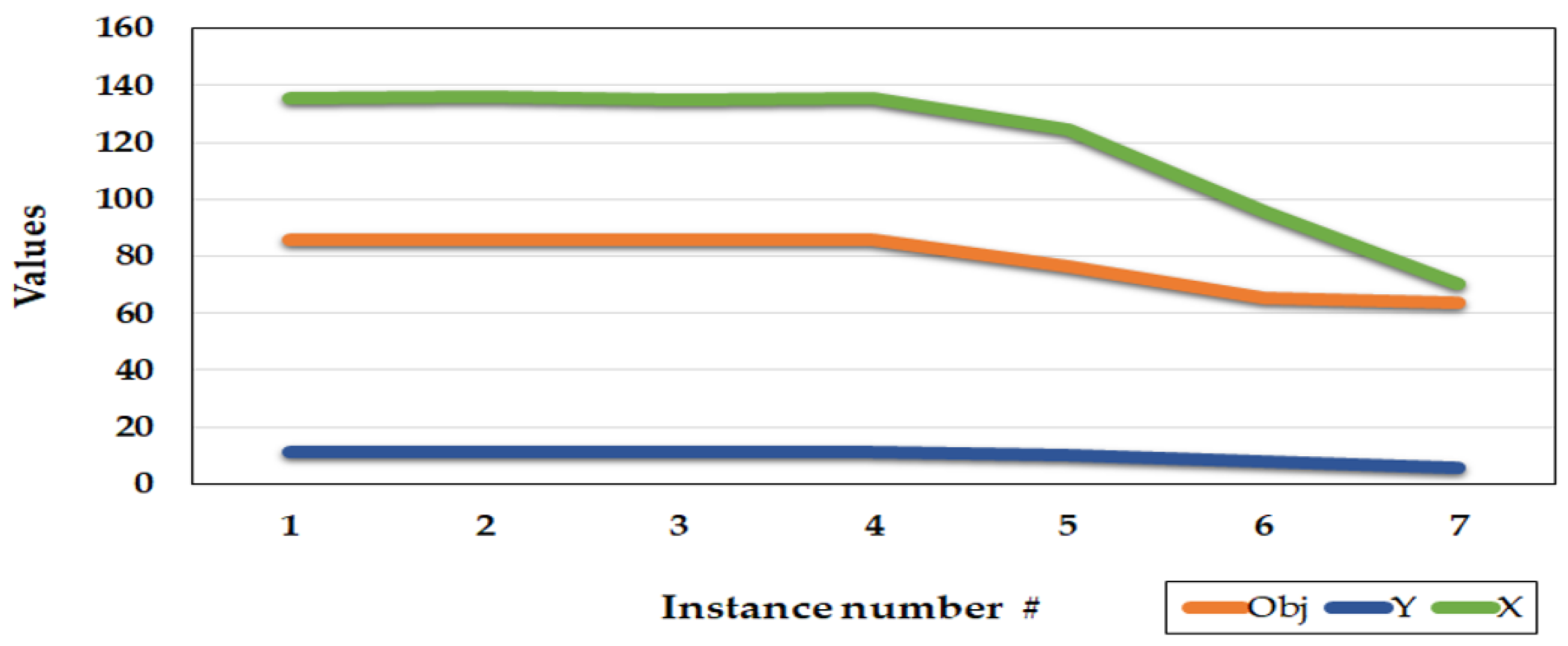
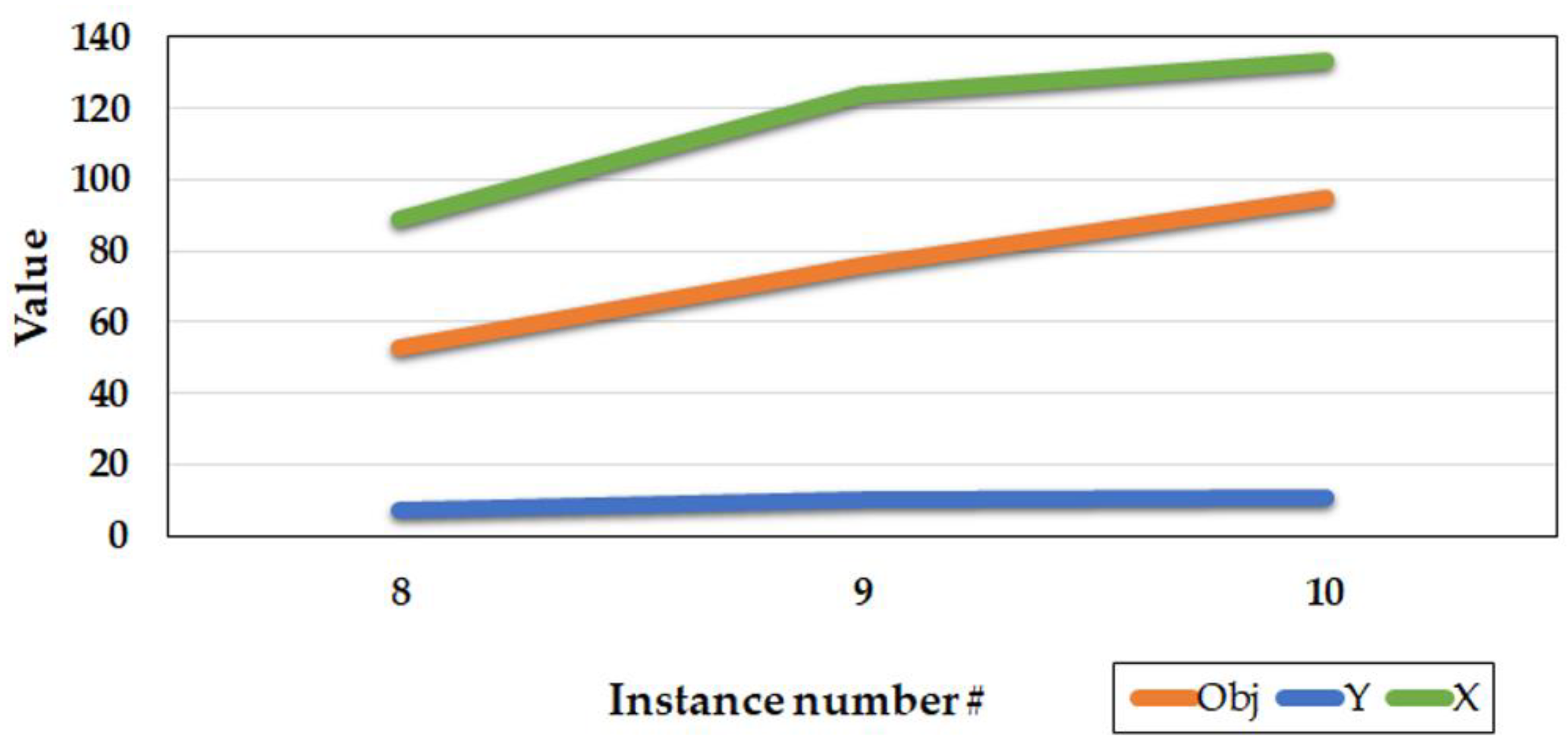
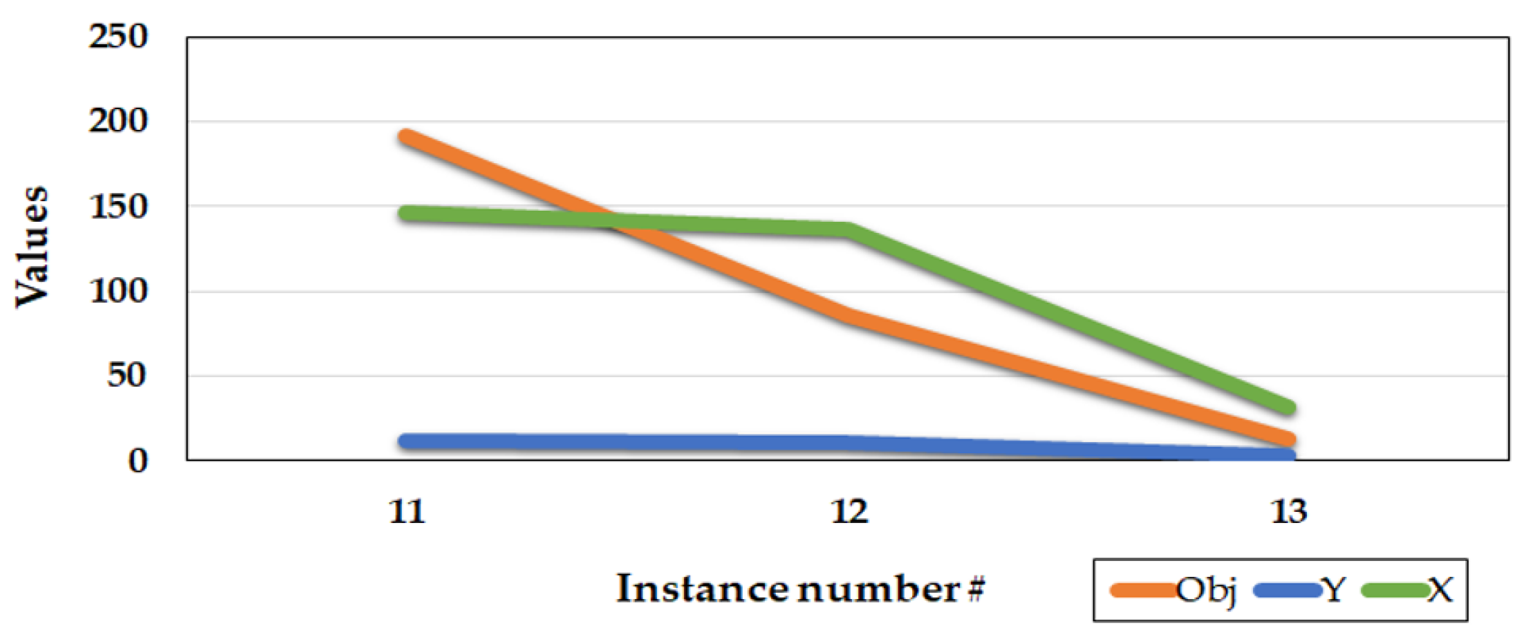
After examining the possible relaxations for the MMCMCLP, different methods are proposed to solve the relaxed and decomposed problems and obtained various upper and lower bounds. Accordingly, a heuristic method is proposed that is able to generate higher lower bounds for the optimal solutions. Although the CPLEX could just solve problems up to 300 demand points, the proposed solution procedures were capable of producing bounds with up to 1000 demand points and 100 potential facilities and beyond. Our results indicate that although common LR problems can still generate upper bounds for complex problems like MMCMCLP, Lagrangian decomposition-based approach combined with the lower bound obtained from developed heuristic methods shows better performance and is preferred to solve for both small- and large-scale problems.
The most important barrier over-performing MMCMCLP for the real application mentioned as disaster relief facility location, hospitals is data insufficiency for the parameters of demands, capacities and costs. To resolve these barriers there is a need to have access to data sets and also applying well-defined demand prediction methods. In addition, a possible future study could be compared using various matheuristics/metaheuristics for this problem, studying the probability of failure and breakdown of modules in different time periods and considering the variable radius coverage for facilities.

Author Contributions

Conceptualization, R.A.; Mathematical model development, R.A., J.B., and M.B.; Methodology, T.N. and R.A.; Software, R.A.; Validation, T.N., J.B., and M.B.; Formal analysis, R.A. and T.N.; Investigation, T.N.; Resources, T.N.; Data Curation, R.A.; Writing—Original Draft Preparation, R.A.; Writing—review and editing, T.N.; Visualization, R.A.; Supervision, T.N., J.B., and M.B.; Project administration, T.N.; Funding acquisition, T.N. All authors have read and agreed to the published version of the manuscript.

Funding

This research was conducted by the aid of the funding provided by JSPS KAKENHI (A) 18H03826.

Institutional Review Board Statement

Not applicable.

Informed Consent Statement

Not applicable.

Data Availability Statement

The data presented in this study are openly available at https://github.com/Alizadehroqayeh/MMCMCLP.

Conflicts of Interest

The authors declare no conflict of interest.

References

  1. Church, R.; ReVelle, C.S. The maximal covering location problem. Pap. Reg. Sci. Assoc. 1974, 32, 101–118. [Google Scholar] [CrossRef]
  2. Moore, G.C.; ReVelle, C.S. The hierarchical service location problem. Manag. Sci. 1982, 28, 775–780. [Google Scholar] [CrossRef]
  3. Farahani, R.Z.; Hekmatfar, M.; Fahimnia, B.; Kazemzadeh, N. Hierarchical facility location problem: Models, classifications, techniques and applications. Comput. Ind. Eng. 2014, 68, 104–117. [Google Scholar] [CrossRef]
  4. Corrêa, F.D.A.; Lorena, L.A.N.; Ribeiro, G.M. A decomposition approach for the probabilistic maximal covering location–allocation problem. Comput. Oper. Res. 2009, 36, 2729–2739. [Google Scholar] [CrossRef]
  5. Pereira, M.A.; Coelho, L.C.; Lorena, L.A.N.; de Souza, L.C. A hybrid method for the probabilistic maximal covering location–allocation problem. Comput. Oper. Res. 2015, 57, 51–59. [Google Scholar] [CrossRef]
  6. Plastria, F.; Vanhaverbeke, L. Discrete models for competitive location with foresight. Comput. Oper. Res. 2008, 35, 683–700. [Google Scholar] [CrossRef]
  7. Fazel Zarandi, M.; Davari, S. The large-scale dynamic maximal covering location problem. Math. Comput. Model. 2013, 57, 710–719. [Google Scholar] [CrossRef]
  8. Yang, P.; Xiao, Y.; Zhang, Y.; Zhou, S.; Yang, J.; Xu, Y. The continuous maximal covering location problem in large-scale natural disaster rescue scenes. Comput. Ind. Eng. 2020, 146, 106608. [Google Scholar] [CrossRef]
  9. Alizadeh, R.; Nishi, T. Dynamic p+q maximal hub location problem for freight transportation planning with rational markets. Adv. Mech. Eng. 2019, 11, 1687814018822934. [Google Scholar] [CrossRef] [Green Version]
  10. Berman, O.; Drezner, Z.; Krass, D. Generalized coverage: New developments in covering location models. Comput. Oper. Res. 2010, 37, 1675–1687. [Google Scholar] [CrossRef]
  11. Farahani, R.Z.; Asgari, N.; Heidari, N.; Hosseininia, M.; Goh, M. Covering problems in facility location: A review. Comput. Ind. Eng. 2012, 62, 368–407. [Google Scholar] [CrossRef]
  12. Balcik, B.; Beamon, B.M.; Krejci, C.C.; Muramatsu, K.M.; Ramirez, M. Coordination in humanitarian relief chains: Practices, challenges and opportunities. Int. J. Prod. Econ. 2010, 126, 22–34. [Google Scholar] [CrossRef]
  13. Beamon, B.M.; Kotleba, S.A. Inventory management support systems for emergency humanitarian relief operations in South Sudan. Int. J. Logist. Manag. 2006, 17, 187–212. [Google Scholar] [CrossRef]
  14. China Pledged to Build a New Hospital in 10 Days. It’s Close. Available online: https://www.nytimes.com/2020/02/03/world/asia/coronavirus-wuhan-hospital.html (accessed on 22 December 2020).
  15. Unique Solution Rolls in to Help Muslims Pray at Tokyo Games. Available online: https://www.japantimes.co.jp/news/2020/02/07/national/muslim-prayer-truck-tokyo-olympics/ (accessed on 22 December 2020).
  16. Baldwin, C.Y.; Clark, K.B. Design Rules: The Power of Modularity; MIT Press: Cambridge, UK, 2000; Volume 1. [Google Scholar]
  17. Hong, Y. A study on the condition of temporary housing following disasters: Focus on container housing. Front. Archit. Res. 2017, 6, 374–383. [Google Scholar] [CrossRef]
  18. Zhang, M.; Zhang, Y.; Qiu, Z.; Wu, H. Two-stage covering location model for air–ground medical rescue system. Sustainability 2019, 11, 3242. [Google Scholar] [CrossRef] [Green Version]
  19. Widener, M.J.; Horner, M.W. A hierarchical approach to modeling hurricane disaster relief goods distribution. J. Transp. Geogr. 2011, 19, 821–828. [Google Scholar] [CrossRef]
  20. Xu, J.; Murray, A.; Wang, Z.; Church, R. Challenges in applying capacitated covering models. Trans. Gis 2020, 24, 268–290. [Google Scholar] [CrossRef]
  21. Manzini, R.; Gebennini, E. Optimization models for the dynamic facility location and allocation problem. Int. J. Prod. Res. 2008, 46, 2061–2086. [Google Scholar] [CrossRef]
  22. Vatsa, A.K.; Jayaswal, S. A new formulation and Benders decomposition for the multi-period maximal covering facility location problem with server uncertainty. Eur. J. Oper. Res. 2016, 251, 404–418. [Google Scholar] [CrossRef]
  23. Marín, A.; Martínez-Merino, L.I.; Rodríguez-Chía, A.M.; Saldanha-da-Gama, F. Multi-period stochastic covering location problems: Modeling framework and solution approach. Eur. J. Oper. Res. 2018, 268, 432–449. [Google Scholar] [CrossRef]
  24. Bagherinejad, J.; Shoeib, M. Dynamic capacitated maximal covering location problem by considering dynamic capacity. Int. J. Ind. Eng. Comput. 2018, 9, 249–264. [Google Scholar] [CrossRef]
  25. Vatsa, A.K.; Jayaswal, S. Capacitated multi-period maximal covering location problem with server uncertainty. Eur. J. Oper. Res. 2020. [Google Scholar] [CrossRef]
  26. Sonego, M.; Echeveste, M.E.S.; Debarba, H.G. The role of modularity in sustainable design: A systematic review. J. Clean. Prod. 2018, 176, 196–209. [Google Scholar] [CrossRef]
  27. Correia, I.; Melo, T. A multi-period facility location problem with modular capacity adjustments and flexible demand fulfillment. Comput. Ind. Eng. 2017, 110, 307–321. [Google Scholar] [CrossRef]
  28. Allman, A.; Zhang, Q. Dynamic location of modular manufacturing facilities with relocation of individual modules. Eur. J. Oper. Res. 2020, 286, 494–507. [Google Scholar] [CrossRef]
  29. Silva, A.; Aloise, D.; Coelho, L.C.; Rocha, C. Heuristics for the dynamic facility location problem with modular capacities. Eur. J. Oper. Res. 2020. [Google Scholar] [CrossRef]
  30. Tanash, M.; Contreras, I.; Vidyarthi, N. An exact algorithm for the modular hub location problem with single assignments. Comput. Oper. Res. 2017, 85, 32–44. [Google Scholar] [CrossRef]
  31. Mikić, M.; Todosijević, R.; Urošević, D. Less is more: General variable neighborhood search for the capacitated modular hub location problem. Comput. Oper. Res. 2019, 110, 101–115. [Google Scholar] [CrossRef]
  32. Keshvari Fard, M.; Alfandari, L. Trade-offs between the stepwise cost function and its linear approximation for the modular hub location problem. Comput. Oper. Res. 2019, 104, 358–374. [Google Scholar] [CrossRef] [Green Version]
  33. Correia, I.; Captivo, M. A Lagrangian heuristic for a modular capacitated location problem. Ann. Oper. Res. 2003, 122, 141–161. [Google Scholar] [CrossRef]
  34. Fathollahi-Fard, A.M.; Hajiaghaei-Keshteli, M.; Tian, G.; Li, Z. An adaptive Lagrangian relaxation-based algorithm for a coordinated water supply and wastewater collection network design problem. Inf. Sci. 2020, 512, 1335–1359. [Google Scholar] [CrossRef]
  35. Hamdan, B.; Diabat, A. Robust design of blood supply chains under risk of disruptions using Lagrangian relaxation. Transp. Res. Part E 2020, 134, 101764. [Google Scholar] [CrossRef]
  36. Zhang, H.; Li, S.; Wang, Y.; Yang, L.; Gao, Z. Collaborative real-time optimization strategy for train rescheduling and track emergency maintenance of high-speed railway: A Lagrangian relaxation-based decomposition algorithm. Omega 2020, 102371. [Google Scholar] [CrossRef]
  37. Nishi, T.; Hiranaka, Y.; Inuiguchi, M. Lagrangian relaxation with cut generation for hybrid flowshop scheduling problems to minimize the total weighted tardiness. Comp. Oper. Res. 2010, 37, 189–198. [Google Scholar] [CrossRef]
  38. Nishi, T.; Shimatani, K.; Inuiguchi, M. Decomposition of Petri nets and Lagrangian relaxation for solving routing problems for AGVs. Int. J. Prod. Res. 2009, 14, 3957–3977. [Google Scholar] [CrossRef]
  39. Ayala, M.; Artigues, C.; Gacias, B. Lagrangian relaxation-based lower bound for resource-constrained modulo scheduling. Electron. Notes Discret. Math. 2010, 36, 191–198. [Google Scholar] [CrossRef]
  40. Yang, Z.; Chen, H.; Chu, F. A Lagrangian relaxation approach for a large scale new variant of capacitated clustering problem. Comput. Ind. Eng. 2011, 61, 430–437. [Google Scholar] [CrossRef]
  41. Litvinchev, I.; Ozuna, E.L. Lagrangian heuristic for the facility location problem. Ifac Proc. Vol. 2013, 46, 107–113. [Google Scholar] [CrossRef]
  42. Diabat, A.; Battaïa, O.; Nazzal, D. An improved Lagrangian relaxation-based heuristic for a joint location-inventory problem. Comput. Oper. Res. 2015, 61, 170–178. [Google Scholar] [CrossRef] [Green Version]
  43. Gendron, B.; Khuong, P.V.; Semet, F. A Lagrangian-based branch-and-bound algorithm for the two-level uncapacitated facility location problem with single-assignment constraints. Transp. Sci. 2016, 50, 1286–1299. [Google Scholar] [CrossRef] [Green Version]
  44. Rafie-Majd, Z.; Pasandideh, S.H.R.; Naderi, B. Modelling and solving the integrated inventory-location-routing problem in a multi-period and multi-perishable product supply chain with uncertainty: Lagrangian relaxation algorithm. Comput. Chem. Eng. 2018, 109, 9–22. [Google Scholar] [CrossRef]
  45. Megiddo, N.; Zemel, E.; Hakimi, S.L. The maximum coverage location problem. Siam J. Algebraic Discret. Methods 1983, 4, 253–261. [Google Scholar] [CrossRef] [Green Version]
  46. Karasakal, O.; Karasakal, E.K. A maximal covering location model in the presence of partial coverage. Comput. Oper. Res. 2004, 31, 1515–1526. [Google Scholar] [CrossRef]
  47. Fisher, M.L. The Lagrangian relaxation method for solving integer programming problems. Manag. Sci. 1981, 27, 1–18. [Google Scholar] [CrossRef]
  48. Geoffrion, A.; Bride, R.M. Lagrangian Relaxation Applied to Capacitated Facility Location Problems. AIIE Trans. 1978, 10, 40–47. [Google Scholar]
  49. Pirkul, H.; Schilling, D. The capacitated maximal covering location problem with backup service. Ann. Oper. Res. 1989, 18, 141–154. [Google Scholar] [CrossRef]
  50. Alizadeh, R.; Nishi, T. Hybrid set covering and dynamic modular covering location problem: Application to an emergency humanitarian logistics problem. Appl. Sci. 2020, 10, 7110. [Google Scholar] [CrossRef]
Figure 1. Illustrative example to depict the modules assignment and facilities location.
Applsci 11 00397 g001
Figure 2. Results of the sensitivity analysis for the capacity of the facilities.
Applsci 11 00397 g002
Figure 3. Results of the sensitivity analysis for the number of the facilities.
Applsci 11 00397 g003
Figure 4. Results of the sensitivity analysis for the module assignment cost.
Applsci 11 00397 g004
Figure 5. Structure of the solving procedures used to obtain bounds.
Applsci 11 00397 g005
Table 1. Investigated studies using different approaches of Lagrangian relaxation method.
AuthorsProblemApproachDecom.Just LB Both LB and UB
Ayala et al. [39]Resource-constrained modular schedulingLR
Nishi et al. [37]Hybrid flowshop scheduling problemLR with cuts
Nishi et al. [38]Automated guided vehicles routing problemLR with Petri nets
Yang, Chen and Chu [40]Large scale new variant of capacitated clustering problemLR approach with two phases of dual optimization
Litvinchev and Ozuna [41]Two-stage capacitated facility location problemLagrangian heuristic producing feasible solutions
Diabat et al. [42]Multi-echelon joint inventory-location problemImproved LR-based heuristics
Gendron et al. [43]Two-level uncapacitated facility location problem with single-assignment constraintsLagrangian-Based Branch-and-Bound Algorithm
Marin et al. [23]Multi-period stochastic covering location problemsLR based algorithm for high quality feasible solutions
Rafie-Majd et al. [44]Three-echelon supply chain integrating inventory-location-routing problem under uncertaintyLR
Hamdan and Diabat [35]Multi-objective and stochastic blood supply chain Lagrangian heuristic
Fathollahi-Fard et al. [34]Coordinated water supply and wastewater collection network design problemAdaptive Lagrangian relaxation-based algorithm
Zhang et al. [36]Train rescheduling and track emergency maintenanceLagrangian-based decomposition
Current researchDynamic modular capacitated maximal covering location problemLagrangian decomposition heuristic
Table 2. Computational results for different values of facility capacity.
# β i ObjYX
1(260,300)85.8111135.6
2(160,200)85.8111136.22
3(100,120)85.8111135.14
4(80,100)85.8111135.46
5(60,80)76.2610124.24
6(50,70)65.6895.53
7(40,60)63.5670.6
Table 3. Computational results to observe the effect of the increasing number of located facilities.
# β i h i l k l t PObjYX
8(60,80)20,40252.9788.9
9(60,80)20,40376.210124.2
10(60,80)20,40494.811133.3
Table 4. Computational results for the effect of the increasing module assignment cost.
# β i h i l k l t PObjYX
11(60,80)10,303191.312146.2
12(60,80)20,40385.8111136.2
13(60,80)30,50313.5332.3
Table 5. Parameter values for the test instances.
# i j t l β i p
1–4101002,33,4(80,100)3
5–8303002,33,4(150,180)12
9–12505003,43,4(200,300)20
13–16707003,43,4(250,350)25
17–2010010003,43,4(300,400)35
Table 6. Computational results to compare CPLEX and the heuristic method.
#CPLEXHeuristic
ObjTimeHLBLO-Gap
1561550.018
2712690.029
3852800.063
411421140
5183833316170.137
6203033818190.116
72847100225740.106
8305650329060.052
Average 0.065
Table 7. Computational results to compare the CPLEX and LR 1 for small size instances.
#CPLEXHeuristicLR1-HLBLR1-LB
ObjTimeHLBUBTimeUO-GapLBUBTimeLO-GapUO-Gap
15615580370.4294775670.1910.339
27126997500.3666894890.0440.324
385280108510.27180110850.0630.294
41142114177540.553101168970.1290.474
51838333161721391730.164164921622840.1150.176
62030338181923122420.139158824655040.2780.214
728471002257432892620.155230134025600.2370.195
83056503290634964090.144236735407340.2910.158
Average 1590.277 3020.1690.272
Table 8. Computational results to compare CPLEX and LR2 for small size instances.
#CPLEXHeuristicLR2-HLBLR2-LB
ObjTimeHLBUBTimeUO-GapLBUBTimeLO-GapUO-Gap
15615572300.2863672400.560.286
27126998330.3806998490.030.380
385280109400.28247109520.810.282
41142114151590.32568117930.6760.026
51838333161722321900.214176422323720.040.214
62030338181923882670.176190723885130.060.176
728471002257433942800.192263433935780.080.192
83056503290636003720.178289436005740.060.178
Average 1580.254 2830.2890.217
Table 9. Computational results to compare CPLEX and LD for small size instances.
#CPLEXHeuristicLD-HLBLD-LB
ObjTimeHLBUBTimeUO-GapLBUBTimeLO-GapUO-Gap
156155521−0.0712451771.333−0.089
27126980510.127-8051 0.127
38528099510.16546102610.8480.200
41142114128520.12333134602.4550.175
51838333161721201480.153158621223330.1590.155
62030338181922801770.123175522802420.1570.123
728471002257431932960.122231731902570.2290.120
83056503290634562750.131263234564530.1610.131
Average 1310.135 1910.7630.147
Table 10. Calculation results to compare the bounds for LR1, LR2, and LD.
#LR1LR2LD
LBUBTimeGapLBUBTimeGapLBUBTimeGap
9247614,0721834.68983211,6306720.18914711,01323560.20
10265313,9373614.25909511,80626400.30-11,102693-
11212218,5322057.73-15,282930--14,429713-
12345318,7463174.4312,31016,00013010.3011,13415,1417900.36
13704721,3054042.02-19,0361941--17,7481620-
14608821,2287662.4912,53419,11718980.53800720,4432871.55
15780828,2535432.62-25,5452157--23,9531548-
16661629,0538443.3918,37226,28228150.4312,74230,4722291.39
1711,11041,3897112.73-37,5174466--35,1234818-
1811,34541,04617842.62-37,7688020--35,9705243-
1914,00254,63613292.90-50,1774759--46,7204870-
2017,82354,47121012.06-50,04321,466--47,3996919-
Average 7953.5 44220.34 25070.87
Table 11. Computational results for fixed lower bound method for LR1, LR2, and LD.
#HeuristicLR1LR2LD
HLBUBTimeGapUBTimeGapUBTimeGap
9794511,67337030.4711,6175850.4611,1184510.40
1010,23711,87048170.1611,8087870.1511,0957750.08
1111,40315,33470160.3415,2836170.3414,3685820.26
1213,81716,02981610.1616,10610930.1715,0567650.09
1312,35818,93573900.5319,30711510.5617,6999690.43
1416,09619,19189720.1919,13925550.1918,06011900.12
1517,68225,21288590.4325,10016940.4224,11312940.36
1623,59026,28921,4290.1126,29524500.1125,66918470.09
1720,74041,38916381.0037,52443540.8135,14328410.69
1829,85737,80637,3810.2737,75854180.2635,93748110.20
1929,62354,64612950.8449,82753440.6846,74938900.58
2037,46954,47151450.4550,03974140.3447,35455670.26
Average 96500.41 27880.37 2081 0.3
Table 12. Best lower bound and upper bound values and methods.
#Best LBBest UB
LBMethodUBMethod
155HLB72LR2-LB = LR2-HLB
269HLB = LR2-LB80LD-HLB = LD-LB
380HLB = LR1-LB99LD-HLB
4114HLB117LR2-LB
51764LR2-LB2120LD-HLB
61907LR2-LB2280LD-HLB = LD-LB
72634LR2-LB3190LD-LB
82906HLB3456LD-HLB = LD-LB
99832LR2-LB11,013LD-LB
1010,237HLB11,095LD-HLB
1111,403HLB14,368LD-HLB
1213,817HLB15,056LD-HLB
1312,464HLB17,699LD-HLB
1416,096HLB18,060LD-HLB
1517,682HLB23,953LD-LB
1623,590HLB25,669LD-HLB
1720,740HLB35,123LD-LB
1829,857HLB35,937LD-HLB
1929,623HLB46,720LD-LB
2037,469HLB47,354LD-HLB
Publisher’s Note: MDPI stays neutral with regard to jurisdictional claims in published maps and institutional affiliations.

