
Air Pollution: Sensitive Detection of PM2.5 and PM10 Concentration Using Hyperspectral Imaging


1
Department of Radiology, Ditmanson Medical Foundation Chia-yi Christian Hospital, Chia-yi City 60002, Taiwan
2
Department of Mechanical Engineering, Advanced Institute of Manufacturing with High Tech Innovations (AIM-HI), and Center for Innovative Research on Aging Society (CIRAS), National Chung Cheng University, 168, University Rd., Min Hsiung, Chia Yi 62102, Taiwan
*
Author to whom correspondence should be addressed.
†
These authors contributed equally to this work.
Appl. Sci. 2021, 11(10), 4543; https://0-doi-org.brum.beds.ac.uk/10.3390/app11104543
Submission received: 11 April 2021
/
Revised: 4 May 2021
/
Accepted: 11 May 2021
/
Published: 17 May 2021
(This article belongs to the Special Issue Innovative and Advanced Applications of Hyperspectral Imaging Technology)
Abstract
:This paper proposes a method to detect air pollution by applying a hyperspectral imaging algorithm for visible light, near infrared, and far infrared. By assigning hyperspectral information to images from monocular, near infrared, and thermal imaging, principal component analysis is performed on hyperspectral images taken at different times to obtain the solar radiation intensity. The Beer–Lambert law and multivariate regression analysis are used to calculate the PM2.5 and PM10 concentrations during the period, which are compared with the corresponding PM2.5 and PM10 concentrations from the Taiwan Environmental Protection Agency to evaluate the accuracy of this method. This study reveals that the accuracy in the visible light band is higher than the near-infrared and far-infrared bands, and it is also the most convenient band for data acquisition. Therefore, in the future, mobile phone cameras will be able to analyze the PM2.5 and PM10 concentrations at any given time using this algorithm by capturing images to increase the convenience and immediacy of detection.
1. Introduction
Hyperspectral remote sensing has been successfully used in various applications, including agriculture, forestry monitoring, food security, natural resources surveying, vegetation observation, geological mapping resource assessment, environmental monitoring, disaster warning, and other remote sensing domains [1,2,3,4,5,6,7,8,9]. Many contemporary studies on air pollution have revealed that air pollution is very harmful to the human body. Air pollution could increase the risk of respiratory and cardiovascular diseases and might even affect the proper functioning of the lungs and proliferate carcinogenesis, whereby normal cells are transformed into cancer cells [10,11,12,13]. Many studies have inferred that suspended PM2.5 (particulate matter with a size of less than 2.5 μm) has a substantial relationship with mortality. Suspended PM2.5 is one of the major causes of non-accidental deaths because of its small size, which enables the particles to penetrate the lung bubbles, directly enery into the blood vessels, and travel along the blood circulation to the entire body [14].
Knowing the concentration of air pollution is imperative for preventing its harmful effects. Most air pollution detection methods are on-the-spot testing methods that examine the extracted air from the atmosphere. Brackx et al. demonstrated a method to assess the potential of hyperspectral tree leaf reflectance in the monitoring of traffic-related air pollution [15]. Elcoroaristizabal et al. fused HSI-NIR and multivariate data analysis in a method validated by thermal–optical transmission analysis to quantify the carbon content in the atmosphere [16]. Manago et al. have developed a method to observe the slant column density of NO2 present in the atmosphere using a concise HSI camera [17]. Although the accuracy of such techniques is often high as they are nearly unsusceptible to external errors and interference, remote air pollution concentration is practically impossible to detect. Ycas et al. used mid-infrared dual-comb spectroscopy technology to detect the quantitative concentration of volatile organic compounds, such as propanol and ethane, in an open path of up to 1 km and measured the released acetone and isoforms with a sensitivity of ppm·m [18]. Phillips et al. also used Open Path–Fourier Transform Infrared technology (OP/FTIR) to detect the influence of the inorganic compound ammonia (NH3) emitted by automobiles [19]. Rutkauskas et al. deployed OP/FTIR technology onto an unmanned aerial vehicle for environmental monitoring using a spectrometer; this approach was able to provide rotational–vibrational spectroscopy over the entire molecular fingerprint area of 3–11 μm [20].
However, the infrared light source used by OP/FTIR has a poor collimation ability, thereby resulting in a low signal-to-noise ratio on long paths. Therefore, Ebner et al. proposed the quantum cascade laser open-path system (QCLOPS) with spectroscopic ellipsometry. Because of the combination of the fast tunability of the QCL and the polarization of the phase modulation, a broadband between 900 and 1024 cm−1 with a high resolution of 1 cm−1 of elliptically polarized spectra can be obtained in less than 1 s [21]. Yin used a continuous wave room temperature, a high-power QCL, and external diffraction grating cavity geometry to develop a sensitive photoelectron sensor system to detect sulfur dioxide (SO2) in the pseudo-units of parts per billion [22]. In addition, Zheng et al. proposed a promising technique for establishing the mass of emanated nitrogen oxide (NO) and other compositions of cigarette smoke [23]. Li et al. developed a piezoelectric effect-based detector based on a broadband tunable external cavity QCL [24]. He et al. developed a detector based on quartz-enhanced photoacoustic spectroscopy, which is a compact, portable and rechargeable sensor platform for the sensitive detection of carbon monoxide (CO) [25].
Although open-path spectrometers, such as OP/FTIR and QCLOPS, can perform the mobile detection of air pollution concentration along a path, they produce large errors due to the poor collimation of the infrared light source. However, this problem is solved by QCLOPS by using a QC laser, which is expensive and difficult to popularize. Foote et al. used an airborne visible/infrared imaging spectrometer (AVIRIS-NG) with a coverage spectrum of 380–2510 nm to collect spectral images and analyze the concentration changes of methane (CH4) over Ahmedabad [26]. Cusworth et al. collected spectral images over California landfills using AVIRIS-NG and used a linearized matched filter algorithm to analyze the distribution of pollutants [27]. In their approach, an imaging spectrometer is equipped with both image and spectrum information and can perform spectrum analysis on a certain area of an image to determine the air pollution concentration and analyze the distribution of pollutants. Therefore, the spectrometers are usually mounted on satellites or unmanned aerial vehicles that acquire a large area of spectrum data from high altitudes for analysis. Nevertheless, this approach uses passive sensing and is expensive, does not have high accuracy, and is thus difficult to employ in daily detection applications.
Although the accuracy of the imaging spectrometer is lower than that of the other two methods above, it can obtain large-area measurements, and its accuracy can be improved with some additional data. Therefore, this study uses hyperspectral images to study air pollution and attempts to develop HSI technology. Cameras that do not originally have spectrum data are assigned spectrum information to significantly reduce the cost of the instrument. Then, the acquired ultra-spectrum images are analyzed for air pollution (i.e., PM10 and PM2.5) to increase the feasibility of daily detection.
2. Theory
2.1. Hyperspectral Image
The fundamentals of spectral imaging are based primarily on the interaction of light with matter [28]. An imaging spectrometer is used on hyperspectral images for imaging in narrow spectral intervals to obtain hyperspectral images in the visible, near-infrared, mid-infrared, and far-infrared bands. Hyperspectral images contain the spatial and spectrum information of the observation scene and consequently the “pattern integration” characteristic. In addition to using the spatial information of the image to determine the location of the area to be detected, it can also use the spectral characteristics of the substances with different chemical compositions [29]. In the application of HSI, the primary wavelength range is visible light to far-infrared light (0.38 μm to 14 μm) and can be divided into two types based on the radiation sources, namely the reflected radiation area (reflected radiation) and emissive radiation area (emissive radiation) [30]. The wavelength range is between 0.38 and 2.5 μm in the reflected radiation, as the main source of radiation is from solar radiation [31,32]. The relationship between the reflectivity (ρ) and emissivity (ϵ) of the substance is shown in Equation (1) [33]:
When a molecule receives solar radiation, it will reflect a part of the solar radiation based on its reflectively. These reflected radiations can be measured by a spectrometer with a wavelength range of 0.38 μm to 2.5 μm, while the emissivity can be measured by a spectrometer with a wavelength of 8 μm to 14 μm. However, in practical applications, the effects of diffuse reflection, scattering, and atmospheric absorption must be considered (see Supplementary Materials for a detailed description of the atmospheric absorption principle). The scattering and absorption effects can be combined into an extinction effect, which can be expressed by the Beer–Lambert law, as shown in Equation (2) [34]:
where I0 is the incident light intensity, I is the light intensity at the required distance, S is the scattering coefficient, K is the absorption coefficient, and S + K is the extinction coefficient (E).
2.2. Air Pollutants of Absorption and Scattering
The air quality standards were created by the Environmental Protection Administration, Executive Yuan through order no. 1010038913 on 14 May 2012, listing fine suspended particulates (PM10), suspended particulates (PM2.5), sulfur dioxide (SO2), nitrogen oxides (NO), carbon monoxide (CO), and ozone (O3) as the main pollutants [35].
- Suspended particles (PM10): Suspended particles with a particle size <10 μm can all be called PM10, and their optical effect is mainly Mie scattering, which is independent of the wavelength—that is, the same proportion of radiation absorption occurs at different wavelengths [36];
- Fine suspended particles (PM2.5): The fine suspended particles among the suspended particles, with a particle size of 2.5 μm, are referred to as PM2.5. The optical effect is Mie scattering, which is not affected by the wavelength, and the proportion of radiation absorption at different wavelengths is the same [36];
- Nitrogen oxides (NOx): NOx mainly includes nitrogen oxide (NO) and nitrogen dioxide (NO2), which also have absorption characteristics in the infrared band. The primary characteristic wavelength of NO is 5.3 μm, while the primary characteristic wavelength of NO2 is 6.2 μm and the secondary characteristic wavelengths are 7.5 μm and 13.3 μm, respectively [39,40];
3. Experiment
The visible HSI (VIS-HSI) used in this study was calculated by using the images taken by a single-lens camera (Nikon D5200, Nikon, Tokyo, Japan) combined with the visible hyperspectral algorithm (VIS-HSA) (see Supplementary Materials for a detailed description of the instrument specification used in this study). The wavelength range was from 380 nm to 780 nm, and the spectral resolution was up to 1 nm. The construction process of this technology is shown in Figure 1. First, the camera and spectrometer (QE65000, Ocean Optics, Dunedin, FL, USA) needed to be provided with numerous common targets for the analysis. If the target could be interpreted within the 380 nm to 780 nm range, then the accuracy of this technology would be improved greatly. In this study, the standard 24-color checker (x-rite classic, 24-color checker) was selected as the target because it contains the most important colors (blue, green, red, grey) and the commonly found colors in nature [42]. To correct the inaccurate white balance generated by the camera, the standard 24-color card needed to be used to obtain a 24-color image (sRGB, 8 bit) and 24-color reflectance spectrum data through the camera and spectrometer, and these were converted to the color space (CIE 1931 color space). The correction coefficient matrix C is shown in Equation (3).
The XYZSpectrum matrix shows the reflection spectrum data converted into the value standardized in the color space, while the variable matrix V is obtained by analyzing the factors that may cause errors in the camera, such as the nonlinear response, dark current, inaccurate color separation, and color shift. The corrected X, Y, and Z (XYZCorrect) values can be obtained from Equation (4), as well as the root-mean-square error of XYZCorrect and XYZSpectrum. The average error was found to be 0.19, which is negligible.
After completing the camera calibration, the 24-color block value (XYZCorrect) obtained from the correction and the 24-color block reflection spectrum data (RSpectrum) measured by the spectrometer could be analyzed to obtain the conversion matrix M. The RSpectrum function was used to determine the principal components through principal component analysis (PCA), and multiple regression analysis was performed on the corresponding principal component scores (PCS) and XYZCorrect. Finally, the above results were integrated to obtain the conversion matrix M. In the multivariate regression analysis of XYZCorrect and the score, the variable VColour was chosen because it lists all possible combinations of X, Y, and Z, and the conversion matrix M is obtained by Equation (5):
Finally, the 24-color block analog spectrum (SSpectrum) was obtained using Equation (6) and compared with the 24-color block reflection spectrum. The root mean square error of each color block was calculated, and the average error was 0.056.
The visible light hyperspectral technology built according to the above process was able to simulate the RGB value captured by a single-lens camera into the reflection spectrum. If the RGB values of the entire image are calculated through the visible light hyperspectral technology, then a visible light hyperspectral image can be obtained (see Supplementary Materials Figure S1 for the NIR Hyperspectral Technology; see Supplementary Materials Figure S2 for the FIR Hyperspectral Technology).
4. Results
4.1. Brightness Correction
Given all-day image capture, the images will be subject to the change of the sun’s tilt angle, meaning that the total brightness of each session would differ, as shown in Figure 2. Therefore, the pre-processing of brightness normalization must be performed. Brightness normalization is still required in the far-infrared band because solar radiation will heat up the object, although it is primarily composed of the heat radiation of the object.
The normalization method of brightness can be achieved through principal component analysis. The first principal component is directly related to the change in solar brightness, while the principal component score is the brightness change coefficient at different times through which the spectral data at different times can be normalized. In this study, 20 locations of the same building in the image were selected for analysis to reduce the concentration changes caused by distance, and the spectrum data of these 20 locations were obtained through HSI technology. Then, these spectrum data were analyzed to obtain correction coefficients for brightness correction. The brightness correction results in the visible light band are shown in Figure 3.
4.2. Regression Analysis
PM2.5 and PM10 primarily exhibit Mie scattering in the visible, near-infrared, and far-infrared bands. Therefore, the spectrum data ware affected by the scattering and exhibit an energy drop. However, the degree of reduction does not change with the wavelength. Thus, the spectrum data are integrated to obtain the variation range and the relationship between the variation range and the concentration of suspended particles according to the Beer–Lambert law and the regression analysis. By integrating the normalized spectrum data of brightness and performing a regression analysis on 2.5 and 10 using Equations (7) and (8) the extinction coefficients of 2.5 and 10 can be obtained. Subsequently, the concentrations of 2.5 and 10 can be obtained using Equations (9) and (10), where RW/OPM is the reflectance that is unaffected by suspended particles.
The result of the regression analysis on the spectrum data in the visible light band for PM2.5 and PM10 is shown in Figure 4. The correlation coefficients for PM2.5 and PM10 were 0.9789 and 0.9738, and the extinction coefficients were 0.005135 and 0.001837, respectively. The correlation coefficient in this band was quite high; that is, the data in this band were highly correlated with the regression equation and had a very close relationship with the suspended particles. The near-infrared HSI (NIR-HSI) used in this study was based on the image of a near-infrared camera and combined with the NIR hyperspectral algorithm (NIR-HSA) (see Supplementary Materials for the regression analysis results of the far-infrared spectrum). The correlation coefficients for PM2.5 and PM10 were 0.6919 and 0.7803, while the extinction coefficients were 0.005765 and 0.003024, respectively. The correlation coefficient in this waveband was lower than that of the visible light waveband; that is, the relationship between the data in this waveband and the suspended particles was less prominent than that in the visible light waveband.
The far-infrared HSI (FIR-HSI) used in this study is based on the image of the thermal imaging camera combined with the FIR hyperspectral algorithm (FIR-HSA; see Supplementary Materials Figure S3 for a detailed description of the FIR-HSI). The correlation coefficients for PM2.5 and PM10 were 1 and , respectively, while the extinction coefficients were 1 and , respectively. Although the correlation coefficient was 1 because the extinction coefficient was quite low, the transmittance was near 1 and could thus be regarded as hardly being affected by the suspended particles (see Supplementary Materials for the estimated results of PM2.5 and PM10 in the FIR and NIR spectra).
4.3. Estimated Results of PM2.5 and PM10
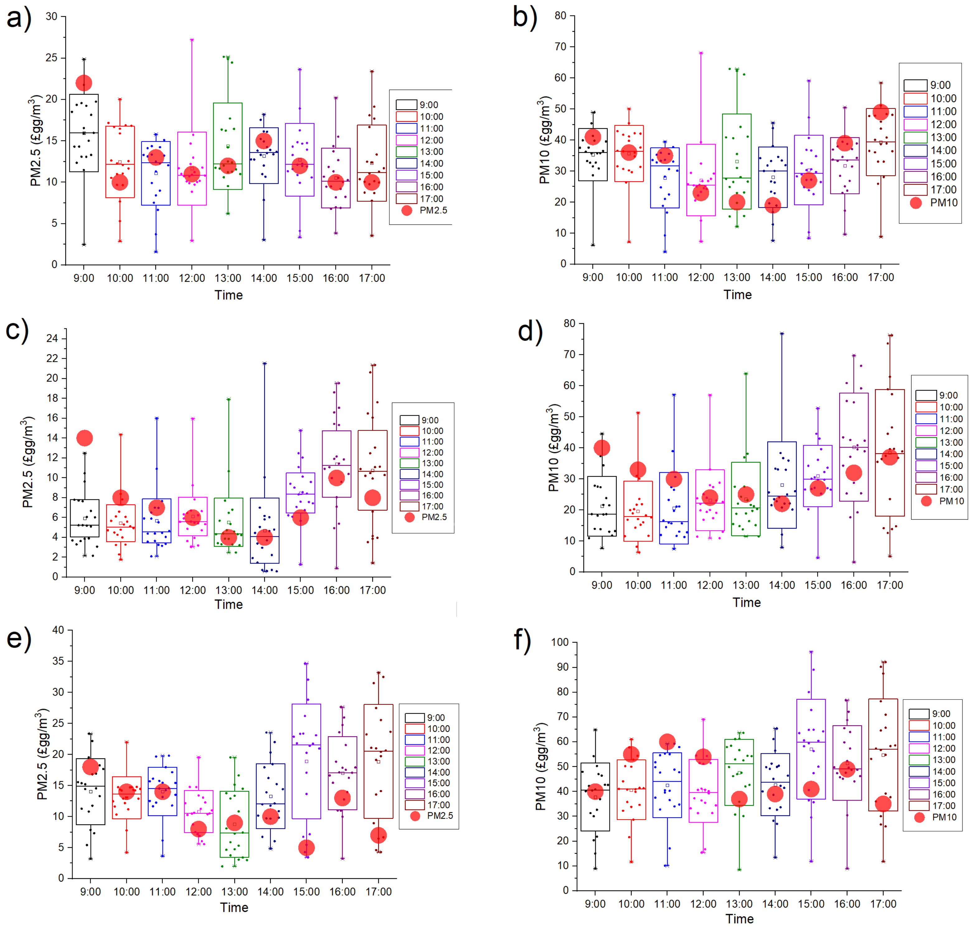
The comparison of the estimated PM2.5 and PM10 concentrations in the visible light band with the data measured by the measuring station is shown in Figure 5 (see Supplementary Materials Figures S4 and S5 for the estimated results of PM2.5 and PM10 in the FIR and NIR spectra respectively). The comparison demonstrates that the visible light band had many concentration values that were evenly scattered around the concentration value of the measuring station, but some deviations remained between the estimated data and the data of the measuring station, which may be attributed to the influence of the environment or sunlight. The above results indicate that the visible light and near-infrared bands are affected by PM2.5 and PM10, while the far-infrared band is unaffected. To understand the calculation error of visible light and near infrared bands, the concentration of suspended particles was measured, and the calculated concentrations were analyzed using the root mean square error. The result is shown in Figure 6, which shows that the error in the visible light band was lower than that in the near infrared band. There are various active methods to reflect a beam from air-suspended solids, such as laser, sonar, and radar; however, in these methods, the acquisition price is high, and it is difficult to interpret the returning output signal independently [43]. In contrast, the passive method discussed in this study is easy to interpret, has no interference problems with the environment, and is cheaper to build.
5. Conclusions
The results of this study show that the PM2.5 and PM10 in the atmosphere have been analyzed in the visible, near-infrared, and far-infrared light bands. In the visible spectrum, the accuracy of detection of PM2.5 and PM10 particulates is higher. The regression analysis of spectral data and particulate matter indicates that the visible light band has a very high correlation coefficient, and accurate results are obtained when estimating the aerosol concentration. Based on the above results, the use of visible light hyperspectral imaging technology to detect air pollution is a better choice than the near-infrared and far-infrared bands, and it is also the most convenient band for data acquisition. During the period of this study, the weather conditions were very good without any particular interference; however, in the future, this method will be tested during various seasons and weather conditions, and an extension of this study would be to use this method with mobile phone cameras to analyze PM2.5 and PM10 at any time by capturing images to increase the convenience and immediacy of detection.
Supplementary Materials
The following are available online at https://0-www-mdpi-com.brum.beds.ac.uk/article/10.3390/app11104543/s1. Figure S1. Near-infrared hyperspectral technology construction process. Figure S2. Far-infrared hyperspectral technology construction process. Figure S3. Detailed description of the FIR-HSI. Figure S4. (a,b) illustrates the estimated results of particulate matter in the NIR band on 13 May 2020. (c,d) represents the estimated results of particulate matter in the NIR band on 28 June 2020. (e,f) shows the estimated results of particulate matter in the NIR band on 29 June 2020. Figure S5. (a,b) illustrates the estimated results of particulate matter in the FIR band on 13 May 2020. (c,d) represents the estimated results of particulate matter in the FIR band on 28 June 2020. (e,f) shows the estimated results of particulate matter in the FIR band on 29/6/2020. Version 3 February 2021 submitted to Sensors 6 of 7.
Author Contributions
Conceptualization, C.-W.C., Y.-S.T. and H.-C.W.; Data curation, C.-W.C., Y.-S.T., A.M. and H.-C.W.; Formal analysis, C.-W.C. and Y.-S.T.; Funding acquisition, C.-W.C., Y.-S.T. and H.-C.W.; Investigation, C.-W.C., Y.-S.T., A.M. and H.-C.W.; Methodology, C.-W.C., Y.-S.T., A.M. and H.-C.W.; Project administration, Y.-S.T. and H.-C.W.; Resources, Y.-S.T.; Software, C.-W.C., Y.-S.T. and A.M.; Supervision, H.-C.W.; Validation, C.-W.C., Y.-S.T., A.M. and H.-C.W.; Writing—Original draft, A.M.; Writing—Review and editing, H.-C.W. and A.M. All authors have read and agreed to the published version of the manuscript.
Funding
This research was supported by the Ministry of Science and Technology, The Republic of China under the Grants MOST 108-2823-8-194-002, 109-2622-8-194-001-TE1, and 109-2622-8-194-007. This work was financially/partially supported by the Advanced Institute of Manufacturing with High-tech Innovations (AIM-HI) and the Center for Innovative Research on Aging Society (CIRAS) from The Featured Areas Research Center Program within the framework of the Higher Education Sprout Project by the Ministry of Education (MOE). This work was also financially/partially supported by the Ditmanson Medical Foundation Chia-Yi Christian Hospital and National Chung Cheng University Joint Research Program (CYCH-CCU-2021-02) in Taiwan.
Institutional Review Board Statement
Not applicable.
Informed Consent Statement
Not applicable.
Data Availability Statement
Not applicable.
Conflicts of Interest
The authors declare no conflict of interest.
References
- Magwaza, L.S.; Opara, U.L.; Nieuwoudt, H.; Cronje, P.J.; Saeys, W.; Nicolaï, B. NIR spectroscopy applications for internal and external quality analysis of citrus fruit—A review. Food Bioprocess Technol. 2012, 5, 425–444. [Google Scholar] [CrossRef]
- Zhang, B.; Wu, D.; Zhang, L.; Jiao, Q.; Li, Q. Application of hyperspectral remote sensing for environment monitoring in mining areas. Environ. Earth Sci. 2012, 65, 649–658. [Google Scholar] [CrossRef]
- Sampson, P.H.; Zarco-Tejada, P.J.; Mohammed, G.H.; Miller, J.R.; Noland, T.L. Hyperspectral remote sensing of forest condition: Estimating chlorophyll content in tolerant hardwoods. For. Sci. 2003, 49, 381–391. [Google Scholar]
- Hou, W.; Wang, J.; Xu, X.; Reid, J.S.; Janz, S.J.; Leitch, J.W. An algorithm for hyperspectral remote sensing of aerosols: 3. Application to the GEO-TASO data in KORUS-AQ field campaign. J. Quant. Spectrosc. Radiat. Transf. 2020, 253, 107161. [Google Scholar] [CrossRef]
- Tong, Q.; Xue, Y.; Zhang, L. Progress in hyperspectral remote sensing science and technology in China over the past three decades. IEEE J. Sel. Top. Appl. Earth Obs. Remote Sens. 2013, 7, 70–91. [Google Scholar] [CrossRef]
- Goetz, A.F. Three decades of hyperspectral remote sensing of the Earth: A personal view. Remote Sens. Environ. 2009, 113, S5–S16. [Google Scholar] [CrossRef]
- Kim, M.S.; Chen, Y.; Mehl, P. Hyperspectral reflectance and fluorescence imaging system for food quality and safety. Trans. ASAE 2001, 44, 721. [Google Scholar]
- Cheng, J.H.; Sun, D.W. Hyperspectral imaging as an effective tool for quality analysis and control of fish and other seafoods: Current research and potential applications. Trends Food Sci. Technol. 2014, 37, 78–91. [Google Scholar] [CrossRef]
- Gomez, R.B. Hyperspectral imaging: A useful technology for transportation analysis. Opt. Eng. 2002, 41, 2137–2143. [Google Scholar] [CrossRef]
- Schraufnagel, D.E.; Balmes, J.R.; Cowl, C.T.; De Matteis, S.; Jung, S.H.; Mortimer, K.; Perez-Padilla, R.; Rice, M.B.; Riojas-Rodriguez, H.; Sood, A. Air pollution and noncommunicable diseases: A review by the Forum of International Respiratory Societies’ Environmental Committee, Part 2: Air pollution and organ systems. Chest 2019, 155, 417–426. [Google Scholar] [CrossRef] [PubMed]
- Lelieveld, J.; Klingmüller, K.; Pozzer, A.; Pöschl, U.; Fnais, M.; Daiber, A.; Münzel, T. Cardiovascular disease burden from ambient air pollution in Europe reassessed using novel hazard ratio functions. Eur. Heart J. 2019, 40, 1590–1596. [Google Scholar] [CrossRef] [PubMed] [Green Version]
- Liu, C.; Chen, R.; Sera, F.; Vicedo-Cabrera, A.M.; Guo, Y.; Tong, S.; Coelho, M.S.; Saldiva, P.H.; Lavigne, E.; Matus, P. Ambient particulate air pollution and daily mortality in 652 cities. N. Engl. J. Med. 2019, 381, 705–715. [Google Scholar] [CrossRef] [PubMed]
- Deryugina, T.; Heutel, G.; Miller, N.H.; Molitor, D.; Reif, J. The mortality and medical costs of air pollution: Evidence from changes in wind direction. Am. Econ. Rev. 2019, 109, 4178–4219. [Google Scholar] [CrossRef] [PubMed]
- Miller, M.R. Oxidative stress and the cardiovascular effects of air pollution. Free Radic. Biol. Med. 2020, 69–87. [Google Scholar] [CrossRef]
- Brackx, M.; Van Wittenberghe, S.; Verhelst, J.; Scheunders, P.; Samson, R. Hyperspectral leaf reflectance of Carpinus betulus L. saplings for urban air quality estimation. Environ. Pollut. 2017, 220, 159–167. [Google Scholar] [CrossRef]
- Elcoroaristizabal, S.; Amigo, J. Near infrared hyperspectral imaging as a tool for quantifying atmospheric carbonaceous aerosol. Microchem. J. 2021, 160, 105619. [Google Scholar] [CrossRef]
- Manago, N.; Takara, Y.; Ando, F.; Noro, N.; Suzuki, M.; Irie, H.; Kuze, H. Visualizing spatial distribution of atmospheric nitrogen dioxide by means of hyperspectral imaging. Appl. Opt. 2018, 57, 5970–5977. [Google Scholar] [CrossRef]
- Ycas, G.; Giorgetta, F.R.; Cossel, K.C.; Waxman, E.M.; Baumann, E.; Newbury, N.R.; Coddington, I. Mid-infrared dual-comb spectroscopy of volatile organic compounds across long open-air paths. Optica 2019, 6, 165–168. [Google Scholar] [CrossRef]
- Phillips, F.A.; Naylor, T.; Forehead, H.; Griffith, D.W.; Kirkwood, J.; Paton-Walsh, C. Vehicle ammonia emissions measured in an urban environment in Sydney, Australia, using open path fourier transform infra-red spectroscopy. Atmosphere 2019, 10, 208. [Google Scholar] [CrossRef] [Green Version]
- Rutkauskas, M.; Asenov, M.; Ramamoorthy, S.; Reid, D.T. Autonomous multi-species environmental gas sensing using drone-based Fourier-transform infrared spectroscopy. Opt. Express 2019, 27, 9578–9587. [Google Scholar] [CrossRef]
- Ebner, A.; Zimmerleiter, R.; Cobet, C.; Hingerl, K.; Brandstetter, M.; Kilgus, J. Sub-second quantum cascade laser based infrared spectroscopic ellipsometry. Opt. Lett. 2019, 44, 3426–3429. [Google Scholar] [CrossRef]
- Yin, X.; Wu, H.; Dong, L.; Li, B.; Ma, W.; Zhang, L.; Yin, W.; Xiao, L.; Jia, S.; Tittel, F.K. ppb-Level SO2 Photoacoustic Sensors with a Suppressed Absorption–Desorption Effect by Using a 7.41 m External-Cavity Quantum Cascade Laser. ACS Sens. 2020, 5, 549–556. [Google Scholar] [CrossRef]
- Zheng, F.; Qiu, X.; Shao, L.; Feng, S.; Cheng, T.; He, X.; He, Q.; Li, C.; Kan, R.; Fittschen, C. Measurement of nitric oxide from cigarette burning using TDLAS based on quantum cascade laser. Opt. Laser Technol. 2020, 124, 105963. [Google Scholar] [CrossRef]
- Li, J.; Liu, N.; Ding, J.; Zhou, S.; He, T.; Zhang, L. Piezoelectric effect-based detector for spectroscopic application. Opt. Lasers Eng. 2019, 115, 141–148. [Google Scholar] [CrossRef]
- He, Y.; Ma, Y.; Tong, Y.; Yu, X.; Tittel, F.K. A portable gas sensor for sensitive CO detection based on quartz-enhanced photoacoustic spectroscopy. Opt. Laser Technol. 2019, 115, 129–133. [Google Scholar] [CrossRef]
- Foote, M.D.; Dennison, P.E.; Thorpe, A.K.; Thompson, D.R.; Jongaramrungruang, S.; Frankenberg, C.; Joshi, S.C. Fast and Accurate Retrieval of Methane Concentration From Imaging Spectrometer Data Using Sparsity Prior. IEEE Trans. Geosci. Remote Sens. 2020, 6480–6492. [Google Scholar] [CrossRef] [Green Version]
- Cusworth, D.H.; Duren, R.M.; Thorpe, A.K.; Tseng, E.; Thompson, D.; Guha, A.; Newman, S.; Foster, K.T.; Miller, C.E. Using remote sensing to detect, validate, and quantify methane emissions from California solid waste operations. Environ. Res. Lett. 2020, 15, 054012. [Google Scholar] [CrossRef]
- Fischer, C.; Kakoulli, I. Multispectral and hyperspectral imaging technologies in conservation: Current research and potential applications. Stud. Conserv. 2006, 51, 3–16. [Google Scholar] [CrossRef]
- Lin, H.; Quan, P.; Wei, D.; Yuan-qing, L. Research Advance on Target Detection for Hyperspectral Imagery. Acta Electron. Sin. 2009, 9, 2016–2024. [Google Scholar]
- Herve, P.; Cedelle, J.; Negreanu, I. Infrared technique for simultaneous determination of temperature and emissivity. Infrared Phys. Technol. 2012, 55, 1–10. [Google Scholar] [CrossRef]
- Manolakis, D.G.; Lockwood, R.B.; Cooley, T.W. Hyperspectral Imaging Remote Sensing: Physics, Sensors, and Algorithms; Cambridge University Press: Cambridge, UK, 2016. [Google Scholar]
- Coakley, J. Reflectance And Albedo, Surface; Oregon State University: Corvallis, OR, USA, 2003; Chapter 9. [Google Scholar]
- Droppleman, J. Apparent microwave emissivity of sea foam. J. Geophys. Res. 1970, 75, 696–698. [Google Scholar] [CrossRef]
- Swinehart, D.F. The beer-lambert law. J. Chem. Educ. 1962, 39, 333. [Google Scholar] [CrossRef]
- Environmental Protection Administration. Air Quality Standards—Taiwan Air Quality Monitoring Network 2012; Environmental Protection Administration: Washington, DC, USA, 2012.
- Eldering, A.; Cass, G.R.; Moon, K. An air monitoring network using continuous particle size distribution monitors: Connecting pollutant properties to visibility via Mie scattering calculations. Atmos. Environ. 1994, 28, 2733–2749. [Google Scholar] [CrossRef]
- Johnson, T.J.; Sams, R.L.; Sharpe, S.W. The PNNL quantitative infrared database for gas-phase sensing: A spectral library for environmental, hazmat, and public safety standoff detection. In Chemical and Biological Point Sensors for Homeland Defense; International Society for Optics and Photonics: Bellingham, WA, USA, 2004; Volume 5269, pp. 159–167. [Google Scholar]
- Nash, D.B.; Betts, B.H. Laboratory Infrared Spectra (2.3–23 m) of SO2 Phases: Applications to Io Surface Analysis. Icarus 1995, 117, 402–419. [Google Scholar] [CrossRef]
- Rothman, L.S.; Gordon, I.E.; Babikov, Y.; Barbe, A.; Benner, D.C.; Bernath, P.F.; Birk, M.; Bizzocchi, L.; Boudon, V.; Brown, L.R. The HITRAN2012 molecular spectroscopic database. J. Quant. Spectrosc. Radiat. Transf. 2013, 130, 4–50. [Google Scholar] [CrossRef] [Green Version]
- Strutt, J.W. On the scattering of light by small particles. Lond. Edinb. Dublin Philos. Mag. J. Sci. 1899, 1, 1869–1881. [Google Scholar]
- Gambacorta, A.; Barnet, C.; Wolf, W.; King, T.; Maddy, E.; Strow, L.; Xiong, X.; Nalli, N.; Goldberg, M. An experiment using high spectral resolution CrIS measurements for atmospheric trace gases: Carbon monoxide retrieval impact study. IEEE Geosci. Remote Sens. Lett. 2014, 11, 1639–1643. [Google Scholar] [CrossRef]
- Pascale, D. RGB Coordinates of the Macbeth ColorChecker; BabelColor Co.: Montreal, QC, Canada, 2006; Volume 6. [Google Scholar]
- Shangari, T.A.; Shams, V.; Azari, B.; Shamshirdar, F.; Baltes, J.; Sadeghnejad, S. Inter-humanoid robot interaction with emphasis on detection: A comparison study. Knowl. Eng. Rev. 2017, 32. [Google Scholar] [CrossRef]
Figure 1.
Visible light spectrum construction process.

Figure 2.
Brightness changes in all the three bands—visible, near-infrared, and far-infrared spectrum—during different parts of the day.
Figure 2.
Brightness changes in all the three bands—visible, near-infrared, and far-infrared spectrum—during different parts of the day.

Figure 3.
(a) The 20 locations selected for spectrum analysis; (b,d,f) the source reflectance at different wavelengths at 9:00, 12:00, and 15:00 GMT+8; (c,e,g) represents same picture after brightness normalization correction. The different colors represent the 20 different locations selected for spectrum analysis.

Figure 4.
The regression analysis results of visible light band spectrum data and particulate matter: (a) PM2.5, (b) PM10.0.
Figure 4.
The regression analysis results of visible light band spectrum data and particulate matter: (a) PM2.5, (b) PM10.0.

Figure 5.
(a,b) The estimated results of particulate matter in VIS on 13 May 2020. (c,d) The estimated results of particulate matter in VIS on 28 June 2020. (e,f) The estimated results of particulate matter in VIS on 29 June 2020.
Figure 5.
(a,b) The estimated results of particulate matter in VIS on 13 May 2020. (c,d) The estimated results of particulate matter in VIS on 28 June 2020. (e,f) The estimated results of particulate matter in VIS on 29 June 2020.

Figure 6.
Expected error of visible light and near infrared bands.

Publisher’s Note: MDPI stays neutral with regard to jurisdictional claims in published maps and institutional affiliations. |
© 2021 by the authors. Licensee MDPI, Basel, Switzerland. This article is an open access article distributed under the terms and conditions of the Creative Commons Attribution (CC BY) license (https://creativecommons.org/licenses/by/4.0/).
Share and Cite
MDPI and ACS Style
Chen, C.-W.; Tseng, Y.-S.; Mukundan, A.; Wang, H.-C. Air Pollution: Sensitive Detection of PM2.5 and PM10 Concentration Using Hyperspectral Imaging. Appl. Sci. 2021, 11, 4543. https://0-doi-org.brum.beds.ac.uk/10.3390/app11104543
AMA Style
Chen C-W, Tseng Y-S, Mukundan A, Wang H-C. Air Pollution: Sensitive Detection of PM2.5 and PM10 Concentration Using Hyperspectral Imaging. Applied Sciences. 2021; 11(10):4543. https://0-doi-org.brum.beds.ac.uk/10.3390/app11104543
Chicago/Turabian StyleChen, Chi-Wen, Yu-Sheng Tseng, Arvind Mukundan, and Hsiang-Chen Wang. 2021. "Air Pollution: Sensitive Detection of PM2.5 and PM10 Concentration Using Hyperspectral Imaging" Applied Sciences 11, no. 10: 4543. https://0-doi-org.brum.beds.ac.uk/10.3390/app11104543
Note that from the first issue of 2016, this journal uses article numbers instead of page numbers. See further details here.