Article

Beef Quality Grade Classification Based on Intramuscular Fat Content Using Hyperspectral Imaging Technology

1
Department of Agricultural and Biosystems Engineering, North Dakota State University, Fargo, ND 58102, USA
2
Department of Animal Science, Sul Ross State University, Alpine, TX 79832, USA
3
Department of Animal Sciences, North Dakota State University, Fargo, ND 58102, USA
4
Engineering Department, University of Jamestown, Jamestown, ND 58405, USA
*
Author to whom correspondence should be addressed.
Submission received: 24 April 2021 / Revised: 9 May 2021 / Accepted: 15 May 2021 / Published: 18 May 2021
(This article belongs to the Special Issue Applications of Hyperspectral Imaging for Food and Agriculture II)

Abstract

:

Featured Application

In this study, hyperspectral imaging was used to evaluate beef quality grades based on their intramuscular fat levels. The results showed the potential of developing an online hyperspectral imaging system for beef quality grading at beef processing plants.

Abstract

Fat content is one of the most important parameters of beef grading. In this study, a hyperspectral imaging (HSI) system, combined with multivariate data analysis, was adopted for the classification of beef grades. Three types of beef samples, namely Akaushi (AK), USDA prime, and USDA choice, were used for HSI image acquisition in the spectral range of 400–1000 nm. Spectral information was extracted from the image by applying the partial least squares discriminant analysis (PLS-DA) for the three classifications. A total of eight different types of data pre-processing procedures were tested during PLS-DA to evaluate their individual performance, with the accepted pre-processing method selected based on the highest accuracy. Chemical and binary images were generated to visualize the fat mapping of the samples. Quantitative analysis of the samples was performed for the reference measurement of the dry matter and fat content. The highest overall accuracy, 86.5%, was found using the Savitzky–Golay second derivatives pre-processing method for PLS-DA analysis. The optimal wavelength values were found from the beta coefficient curve. The chemical and binary images showed significant differences in fat mapping among the three groups of samples, with AK having the greatest intramuscular fat content and USDA choice having the least. Similar results were observed during the proximate analysis. The findings of this study demonstrate that the HSI technique is a potential tool for the fast and non-destructive determination of beef grades based on fat mapping.

1. Introduction

Meat from beef, pork, lamb, and goat is an important dietary source of protein, vitamins, and minerals necessary for optimal human health [1]. In the past decade, the production and consumption of meat has continually increased due to customer demand [2]. As income levels increase, the interest in meat quality, meat safety, and animal welfare also increases [3]. When consumers purchase beef products, the primary factors driving the purchase decisions are price, color, and fat, which are the key points of beef grading [4]. The amount and type of fat content play a vital role during beef grading, which also has a great influence on the consumer choice and the price of beef [5].
Beef grading plays an important role not only in the beef industry, but also for the consumers. The beef quality and grading have a straightforward relationship, which is intensely critical to the business transactions, marketing, and buyer choice during selling or purchasing. The United States Department of Agriculture (USDA) established beef grading based on the intramuscular fat content and the maturity level of the beef [6]. Based on the USDA grading standard, the commercial beef grades are prime, choice, and select. Prime beef contains abundant marbling (intramuscular fat) and is produced from young and well-fed beef cattle. Choice beef is also high-quality beef but contains less marbling compared to prime beef. Another type of beef called Akaushi (AK) is produced from Akaushi beef cattle, which was created by the Japanese Association of Akaushi as a premium beef breed. Prime beef produced from Akaushi has great value due to its enhanced quality and plentiful amount of marbling. Beef palatability and marbling have a strong interconnection that has been established for decades [7,8,9,10,11]. Hence, marbling in beef is considered a major parameter for beef grading. In the standard method, meat fat is determined by the solvent extraction of the total lipids followed by the conversion of fatty acids to their methyl esters, and the final analysis is performed by gas chromatography [12]. This method requires time and chemicals and is a high-cost procedure, which are drawbacks for routine analysis. However, for beef grading, a subjective characteristic assessment is performed by highly skilled USDA meat graders and the meat attributes are measured using electronic instruments [13]. This process is subjective and requires expert-level knowledge. Therefore, the development of an accurate, objective, automated system that can give instantaneous results to grade beef, based on the marbling content, would revolutionize the industry. This is where HSI, in combination with machine learning, can be a potential option.
Research, development, and application of machine vision technology in the food and meat industry has grown rapidly with increased public expectations for high-quality, palatable, and safe food products. Automated computer vision systems possess great potential for fast, objective, no-contact quality control and food safety inspection [14]. Hyperspectral imaging is a potential non-destructive computer vision technique that has been adopted for the product quality analysis of meat [15], fish [16], dairy foods [17], grain [18], lettuce [19], and green citrus [20]. Xiong et al. found that HSI was a powerful technique for predicting quality attributes commonly evaluated in red meats, including lean color, intramuscular pH, marbling, tenderness, chemical composition, water-holding capacity, and microbial spoilage [1]. Previously, Li et al. observed that HSI analyses performed in the spectral range of 400 to 1100 nm were able to predict 92% of the variation in beef marbling [21]. While these results are promising, there is limited research focused on using HSI to evaluate marbling levels for beef grading.
Therefore, the objective of this research was to evaluate the potential of using HSI for beef grading based on marbling levels. In this study, three classes of beef, namely Akaushi (AK), USDA prime, and USDA choice, were used. Additionally, proximate analyses (dry matter and intramuscular fat content) were performed to verify the differences between the quality grades and the obtained HSI results.

2. Materials and Methods

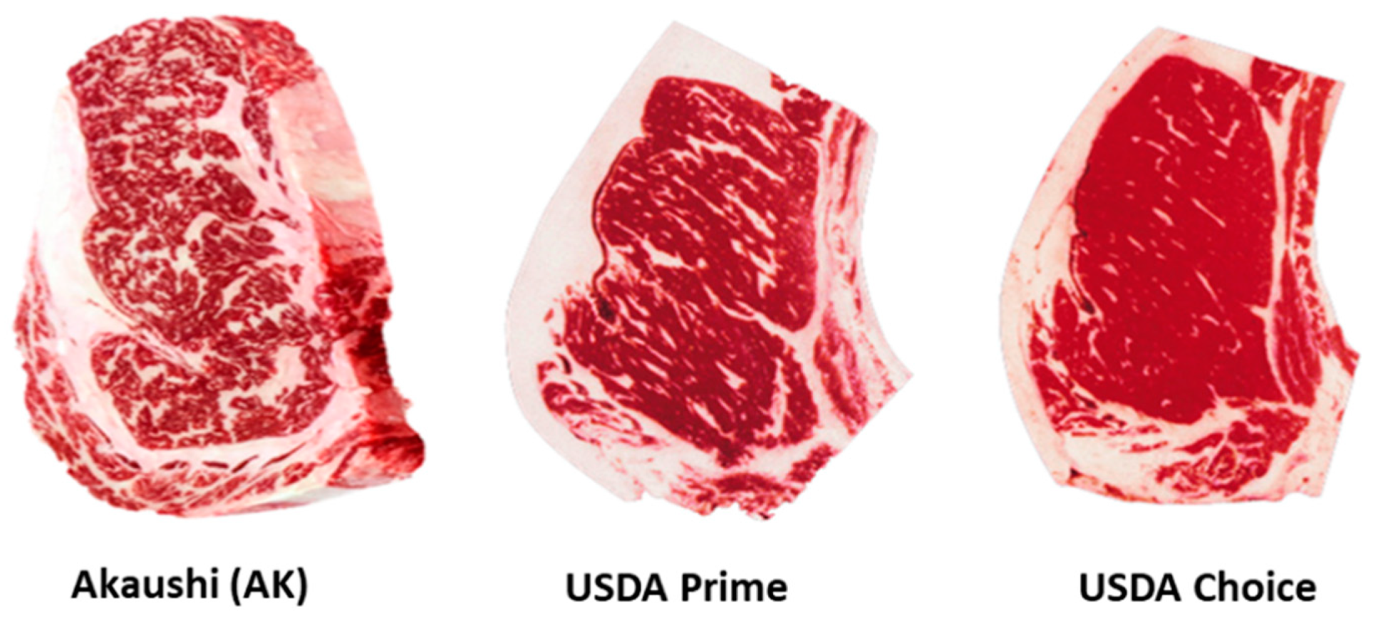
2.1. Collection of Beef Samples

Boneless beef ribeye roll, lip-on subprimals (IMPS 112A) were utilized for analyses. Vacuum-packaged USDA prime (n = 30) and USDA choice (n = 30) quality grade ribeye rolls were purchased from the local Costco Wholesale Meat Department (Fargo, ND, USA), transported approximately 13 km to the North Dakota State University Meat Laboratory (NDSU Meat Lab., Fargo, ND, USA) at ambient temperature, and stored at 2 °C. Ribeye rolls (n = 30) from Akaushi (AK) steers, marketed under the HeartBrand Beef Inc. brand (Flatonia, TX, USA), were collected from the fabrication line of Caviness Beef Packers (Hereford, TX, USA), a commercial beef processor. Rolls were vacuum-packaged, transported approximately 1400 km to the NDSU Meat Lab on ice, and stored at 2 °C. The samples were aged for 14 days at 2 °C, after which the ribeye rolls were fabricated from the anterior end into 2.54 cm steaks (Figure 1). The chopped steaks were placed into trays with their identification number and assigned analyses were conducted. From each class, 30 steaks (a total of 90 steaks from the 3 classes) were utilized for hyperspectral image acquisition.

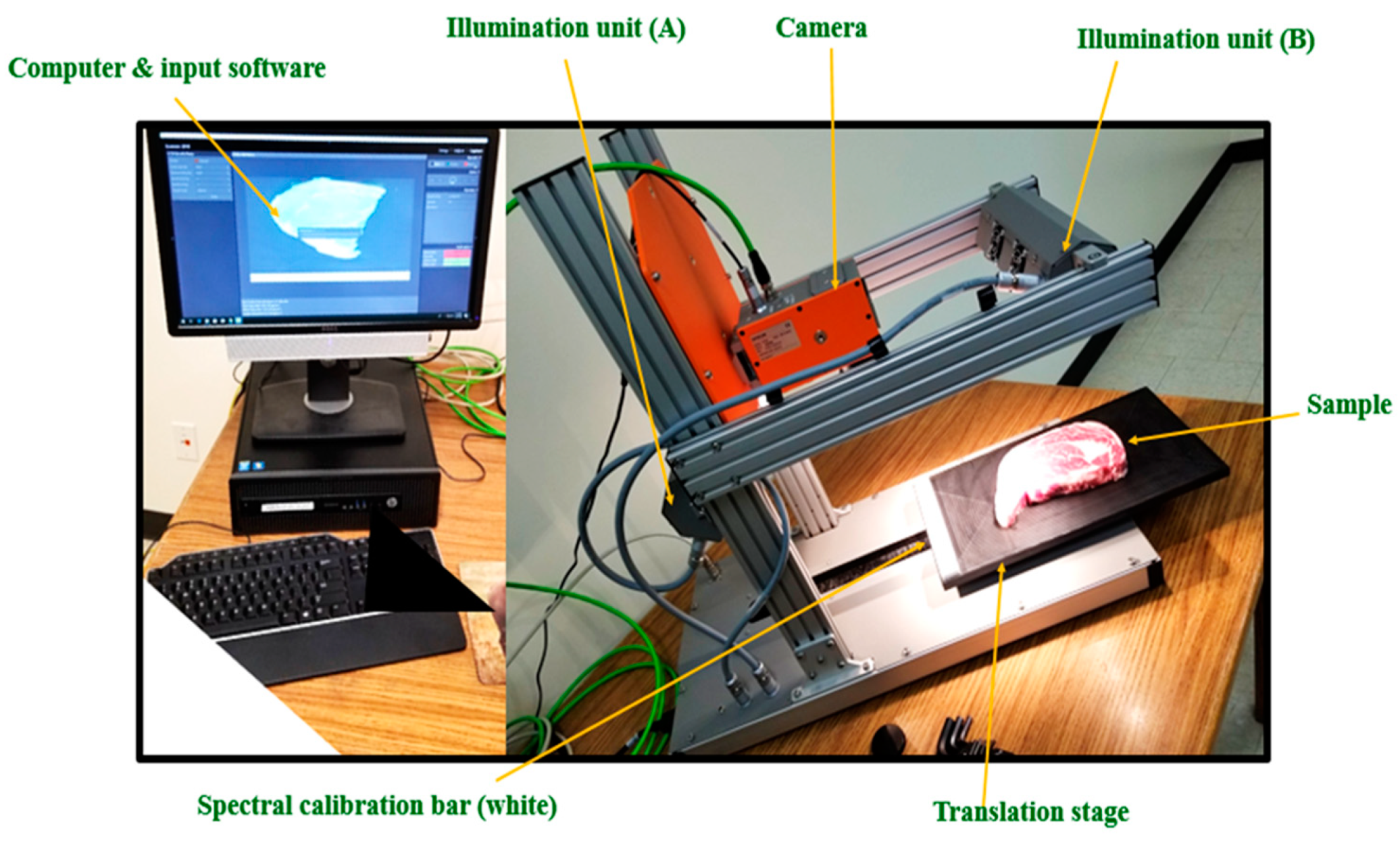
2.2. Hyperspectral Image Acquisition

A lab-based visible-near-infrared HSI system was used in reflectance mode for HSI acquisition. The wavelength range of the HSI sensor was 400–1000 nm. The HSI system consisted of four main parts: (1) the camera (Specim FX 10e, Middleton Spectral Vision; Middleton, WI, USA); (2) illumination system (Via-Spec™ II Halogen Reflectance Illumination-MRC-920-045); (3) sample conveying acquisition system (Lab Scanner Setup 40 × 20-MRC-313-004-05); and (4) the Lumo Scanner software, which allows the user to set up, adjust, and acquire data for the supported Specim spectral camera. Figure 2 shows the essential parts and units of the designed HSI system.
The 90 samples used for the HSI analysis were placed on the sample base and conveyed to the camera sensor for capturing the image by line scanning. Before image acquisition, each steak was allowed to bloom (oxymyoglobin formation) for 20 min after cutting from the ribeye roll sub-primal. All images were subjected to a complete set of image interrogation and analysis tools to aid the imaging process. The collected resolution of each HSI spectral image was 1024 × 2056 pixels on 448 bands. Considering the signal-to-noise ratio, the conveyor platform speed was set to 28 mm/s and the distance between the sample and the camera lens was 25.5 cm. For system calibration, a Teflon bar (20 × 2 cm) with ~99% reflectance (white) area was first placed on the scanning bed and captured as a calibration image. The following equation was used to calibrate the hyperspectral images:
I = I 0 D W D
where I is the calibrated image, I0 is the raw hyperspectral image, W represents a mean value of the white reference, and D represents a mean value of the dark reference.

2.3. Quantitative Analyses

After completing the HSI image acquisition, samples were stored at 2 °C for proximate analyses to evaluate the dry matter and intramuscular fat content. A 4 × 8 cm rectangle was cut from the center of each steak and sealed in Whirl-Pak® (Madison, WI, USA) bags. The samples were sent to the University of Missouri Experiment Station Chemical Laboratories (Columbia, MO, USA) for proximate analysis. The official methods of cation-exchange chromatography coupled with post-column ninhydrin derivatization and quantitation, following the Association of Official Analytical Chemists (AOAC) guidelines, were used for the proximate analyses. Later, the statistical analyses (analysis of variance test (ANOVA)) were conducted using SAS (v. 9.4, SAS Institute, Inc., Cary, NC, USA) to analyze the intramuscular fat and dry matter content of the samples.

2.4. Spectral Extraction

During image acquisition, some random spatial noises were generated due to light heat and ambient conditions. A 3 × 3 window median filter was applied on each band image to reduce the noise. Later, the region of interest (ROI) was manually selected using the 662 nm band image and spectral information was extracted from the respective beef samples’ HSI images [18]. The mean of the collected spectral data was saved according to the sample’s number, resulting in 30 mean spectra from each class of samples (a total of 90 from the 3 classes). From individual classes, 70% of the spectral data were used for calibration, and 30% were used for validation during model development.

2.5. Data Pre-Processing

Pre-processing is an important task to reduce the effect of asymmetries in the spectral data, which may occur due to noise, light scattering, sample texture, and ambient temperature. Pre-processing improves the data quality to enhance the model performance. In this study, eight different types of pre-processing were applied to the spectral data: mean normalization, maximum normalization, range normalization, multiplicative scatter correction (MSC), standard normal variate (SNV), Savitzky–Golay first derivatives, Savitzky–Golay second derivatives, and data smoothing. Normalization pre-processing fits the spectral data in a similar range, while SNV and MSC remove slope differences and unwanted scatter effectsSavitzky–Golay derivatives improved the spectral resolution by removing the baseline offsets and overlapping peaks. Sometimes, the noise arising from the instruments can be resolved by using a data smoothing filter [22,23,24,25,26].

2.6. Model Development

The pre-processed data from each pre-processing method were used to develop a partial least squares discriminant analysis (PLS-DA) multivariate model to classify the 3 categories of beef samples. PLS-DA is a powerful multivariate data analysis tool that is modified from a partial least square regression (PLS-R) and was used for spectral and hyperspectral imaging in earlier studies [27,28]. The relationship between the data matrix and the response matrix is revealed by this method. Initially, a transformation of the data matrix generates a set of intermediate linear latent variables, which is used for regression with the response matrix. The final regression/beta coefficients can be applied to predict a new or unknown samples data matrix. PLS-DA is generally expressed as:
Y = X × b + E ,
where X = n × p that holds the spectral values of each class, b is the regression coefficient, and E is the error term. To develop the model, the spectral data of all groups were arranged in a matrix X and the calculated values were entered into the Y matrix as:
Y = { 1 = sample   belongs   to   AK 2 = sample   belongs   to   USDA   prime 3 = sample   belongs   to   USDA   choice
To develop the linear relationship between the predictors and response variables, both X and Y values were changed by latent variables (LVs):
X = TP T + E X
Y = UQ T + E Y
Here, P and Q represent the loading matrix, and T and U represent the score matrix. EX and EY are the residual matrices of X and Y, respectively.
Due to the effectiveness of producing a robust result for multivariate data analysis, the PLS method is the most commonly applied technique in chemometrics [29].

2.7. Image Processing

From the studied data pre-processing methods, the accepted method was selected based on the highest accuracy. Afterwards, the chemical image was generated by the multiplication of the beta coefficients and the original masked HSI image. The generated chemical image was converted into a binary image using a threshold value with 1 considered as fat and 0 as lean. Based on the extent of the pixel value 1, the beef samples were classified according to their grade. Except for HSI image acquisition, all of the operations were executed by using MATLAB (2018a, MathWorks, Natick, MA, USA) based on a custom built algorithm.

3. Results and Discussion

3.1. Hyperspectral Imaging

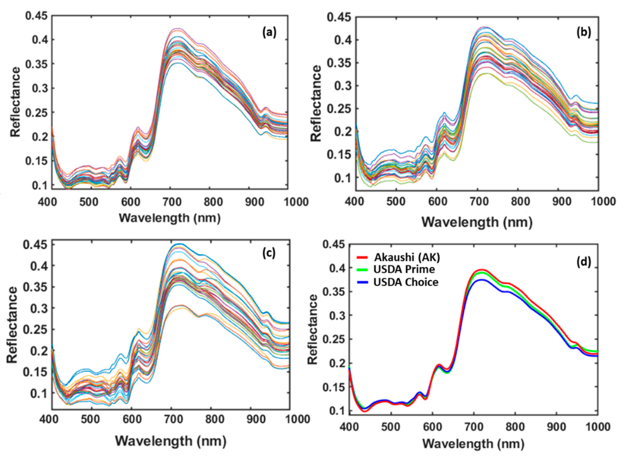
3.1.1. Spectral Data Interpretation

Original spectra were collected from the selected ROI of each sample from 397 nm to 1004 nm. Therefore, 30 spectra from each group were obtained and plotted for the individual classes shown in Figure 3a–c. The spectral pattern was similar for all three classes. Figure 3d shows the mean spectra for each class, where AK exhibited the highest reflectance in comparison to the other groups from 680 nm to 1000 nm. However, USDA prime had a higher reflectance than USDA choice in the same region. The spectral reflectance is highly correlated with the fat and lean content of the beef. Generally, fat reflects the light more than lean content because of its color and chemical content [3].

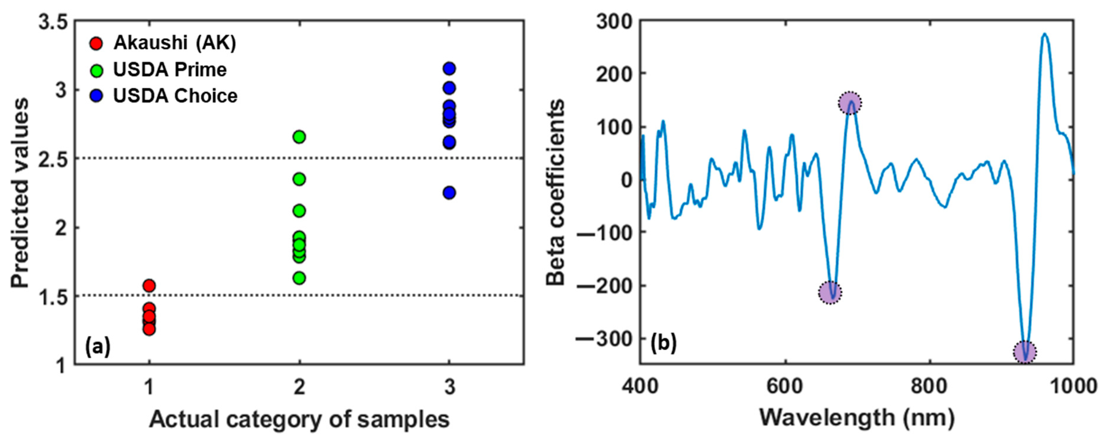
3.1.2. PLS-DA Model Results

PLS-DA was performed to build the classification model. PLS-DA was suitable because the predictors had more variables than the observations and a high level of correlation was present among the original predictors [30]. The classification results of the PLS-DA, after applying pre-processing methods, are presented in Table 1. The Savitzky–Golay second derivatives performed the best, producing the highest overall accuracy of 86.5% using five latent variables, as Savitzky–Golay pre-processed spectra always give more accurate spectral information [31]. Latent variables were calculated from the prediction set of the classification model considering the lower error rate, which is a common practice to evaluate the classification model performance [32].
The multivariate analysis of the PLS-DA model for beef classification according to the grade is illustrated in Figure 4, where Figure 4a is the beef classification group after applying the Savitzky–Golay second pre-processing method and Figure 4b is the beta coefficient curve obtained from the developed PLS-DA model. The computed values entered into the Y matrix were 1, 2, and 3 for AK, USDA prime, and USDA choice, respectively; therefore, the threshold value to separate AK and USDA prime was 1.5 and the value to separate USDA prime and USDA choice was 2.5. Some samples were found to be misclassified in each group (Figure 4a). Two AK samples were misclassified as USDA prime, one USDA prime sample as USDA choice, and one USDA choice as USDA prime based on their threshold values. However, no USDA prime or USDA choice samples were misclassified as AK. This misclassification may have happened due to the temperature difference during spectral acquisition or vibration of the sample holder. After the classification, samples were visually inspected according to their respective sample numbers. The fat profile of the misclassified samples was observed carefully, and it was found that the AK samples showed some similarity with the USDA prime sample, and the USDA choice showed similarity with the USDA prime, which may explain the misclassification.
The beta coefficient developed from the PLS-DA model (Figure 4b) can be used for informative wavelength selection and interpretation of results. To interpret the multivariate data analysis results, the beta coefficient curve provides significant information related to the particular peak difference and wavelength selection, which is important to minimize the excessive information from the HSI images and optimize the final classification system [16]. The observed peak of the developed beta coefficient curve for the prediction of the chemical components matched with the spectral information of previously published research [33,34]. The highest absolute values of the beta coefficient were observed at 657 nm, 701 nm, and 932 nm wavelengths (marked with violet circles), which are responsible for the classification and the interpretation of the model. The first two wavelengths were important to visualize the fat mapping of the beef samples that agreed with the Lohumi et al. study to identify intramuscular fat distribution [3]. The waveband at 932 nm is responsible for the third overtone of the C–H stretching, which is related to the presence of fat in the muscle [35]. Similar spectral information in the selected waveband was found by the Kandpal et al. study for fat profile of the beef [2].

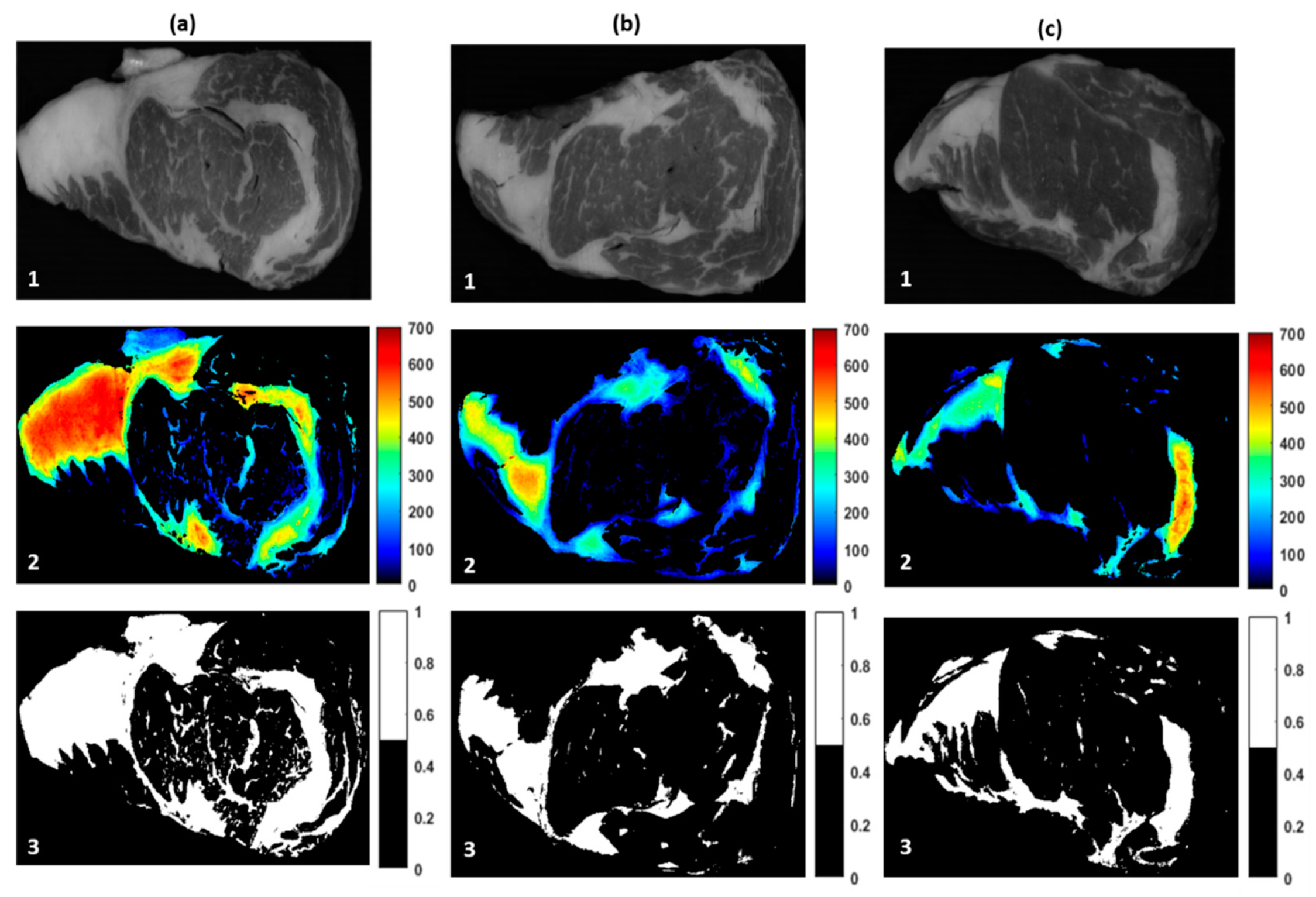
3.1.3. Fat Profile Prediction and Visualization

The chemical images (PLS images) of the samples were generated by applying the accepted beta coefficients to the masked 3D data HSI images (Figure 5, row 1). This operation produced a classification image of the samples, which can visualize the fat content map of the samples. Previous research also used similar methodology to visualize corn viability [22] and almond adulteration detection [36]. Figure 5, row 2 shows the chemical images of the three samples from the three different classes. The difference among the three groups is significantly evident in the fat part of the samples, as predicted by the beta coefficient plot. For clear observation of the fat mapping in the samples, a binary classification model of the samples was also generated. The binary images (Figure 5, row 3) represented the fat part as pixel value 1 (white) and the lean and background as pixel value 0 (black). Fat content of the samples was evaluated considering the white part of the images and this information was used to classify the three grades of the beef samples. From the PLS image, the difference among the three groups is significantly evident in the fat content regions of the samples, as predicted by the peaks in the beta coefficients plot (Figure 5, row 3). Hence, the developed PLS-DA model-based image analysis performed satisfactorily to classify the beef steaks based on the fat profile.

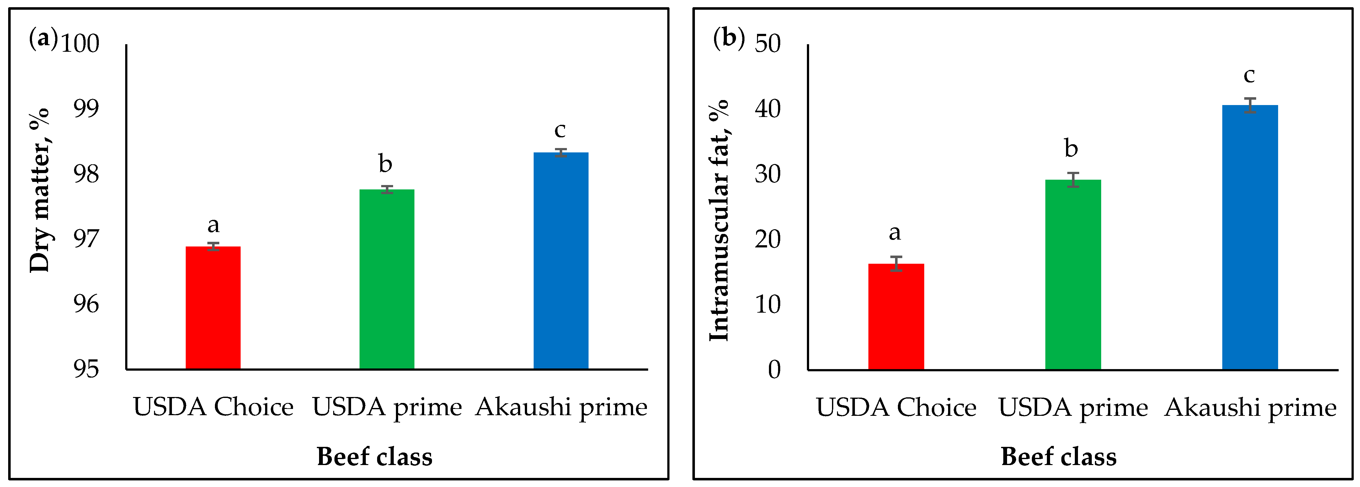
3.2. Quantitative Analysis

Proximate analysis was performed as a reference measurement of the fat and dry matter content of the samples from the three different classes. Both dry matter percentage and intramuscular fat percentage showed significant differences (p < 0.0001) between classes (Figure 6). Dry matter content increased from USDA choice to USDA prime to AK (96.9%, 97.8%, and 98.3%, respectively). The highest intramuscular fat content was observed in AK (40.64%), followed by USDA prime (38.29%) and USDA choice (37.56%) samples.

4. Conclusions

Fat content in beef is an important factor for the grading procedure. Akaushi beef had the greatest amount of intramuscular fat while USDA choice had the least. This was supported by HSI, which showed that AK beef had more pixels classified as fat compared to USDA prime or USDA choice. Additionally, this study found that the best wavelength range for evaluating intramuscular fat content was 650–950 nm. Overall, this study showed great potential for using HSI as a classification technique for fast, reliable, and noninvasive beef grading.

Author Contributions

D.D.R.J. conceived the study and performed the experiments. M.R.A., S.E., and D.D.R.J. performed the image data analysis and wrote the paper. J.M.Y. conducted the statistical analysis of the quantitative analyses data and reviewed and edited the manuscript. X.S. reviewed and edited the manuscript. X.S. and E.P.B. acquired the funding for this research. All authors have read and agreed to the published version of the manuscript.

Funding

This research was supported by North Dakota Beef Commission (project number FAR0027501).

Institutional Review Board Statement

Not applicable.

Informed Consent Statement

Not applicable.

Data Availability Statement

The data presented in this study are available on request from the corresponding author. The data are not publicly available due to the date size and format.

Acknowledgments

The authors would like to thank the team members that assisted with data collection: J. Liu, C. Lee, J Dubbels, S. Taves, K. Gunderson, and J. Quanbeck. West Texas A&M University and T. Lawrence hosted our sample collection team when travelling to Texas to pick up the Akaushi samples. NDSU’s Meat Lab staff and S. Wirt (manager) for hosting sample breakdown and sample storage.

Conflicts of Interest

The authors declare that there are no conflicts of interest regarding this research and publication of this manuscript.

References

  1. Xiong, Z.; Sun, D.W.; Zeng, X.A.; Xie, A. Recent developments of hyperspectral imaging systems and their applications in detecting quality attributes of red meats: A review. J. Food Eng. 2014, 132, 1–13. [Google Scholar] [CrossRef]
  2. Kandpal, L.; Lee, J.; Bae, J.; Lohumi, S.; Cho, B.-K. Development of a Low-Cost Multi-Waveband LED Illumination Imaging Technique for Rapid Evaluation of Fresh Meat Quality. Appl. Sci. 2019, 9, 912. [Google Scholar] [CrossRef] [Green Version]
  3. Lohumi, S.; Lee, S.; Lee, H.; Kim, M.S.; Lee, W.H.; Cho, B.K. Application of hyperspectral imaging for characterization of intramuscular fat distribution in beef. Infrared Phys. Technol. 2016, 74, 1–10. [Google Scholar] [CrossRef]
  4. Font-i-Furnols, M.; Guerrero, L. Consumer preference, behavior and perception about meat and meat products: An overview. Meat Sci. 2014, 98, 361–371. [Google Scholar] [CrossRef]
  5. Lusk, J.L.; Parker, N. Consumer Preferences for Amount and Type of Fat in Ground Beef. J. Agric. Appl. Econ. 2009, 41, 75–90. [Google Scholar] [CrossRef] [Green Version]
  6. Carriquiry, M. Guaranteed Tender Beef: Opportunities and Challenges for a Differentiated Agricultural Product. Cent. Agric. R. Dev. Iowa State Univ. Work. Pap. 2004, 371, 1–18. [Google Scholar]
  7. Blumer, T.N. Relationship of Marbling to the Palatability of Beef. J. Anim. Sci. 1963, 22, 771–778. [Google Scholar] [CrossRef]
  8. Westerling, D.B.; Hedrick, H.B. Fatty Acid Composition of Bovine Lipids as Influenced by Diet, Sex and Anatomical Location and Relationship to Sensory Characteristics. J. Anim. Sci. 1979, 48, 1343–1348. [Google Scholar] [CrossRef]
  9. Savell, J.W.; Branson, R.E.; Cross, H.R.; Stiffler, D.M.; Wise, J.W.; Griffin, D.B.; Smith, G.C. National Consumer Retail Beef Study: Palatability Evaluations of Beef Loin Steaks that Differed in Marbling. J. Food Sci. 1987, 52, 517–519. [Google Scholar] [CrossRef]
  10. Wheeler, T.L.; Cundiff, L.V.; Koch, R.M. Effect of marbling degree on beef palatability in Bos taurus and Bos indicus cattle1. J. Anim. Sci. 1994, 72, 3145–3151. [Google Scholar] [CrossRef] [PubMed]
  11. Smith, S.B. Marbling and Its nutritional impact on risk factors for cardiovascular disease. Korean J. Food Sci. Anim. Resour. 2016, 36, 435–444. [Google Scholar] [CrossRef] [PubMed] [Green Version]
  12. Aldai, N.; Kramer, J.K.G.; Cruz-Hernandez, C.; Santercole, V.; Delmonte, P.; Mossoba, M.M.; Dugan, M.E.R. Appropriate extraction and methylation techniques. In Fat and Fatty Acids in Poultry Nutrition and Health; Cherian, G., Poureslami, R., Eds.; Context Products Ltd.: Leicestershire, UK, 2012; pp. 249–278. [Google Scholar]
  13. USDA. What’s Your Beef–Prime, Choice or Select? USDA. Available online: https://www.usda.gov/media/blog/2013/01/28/whats-your-beef-prime-choice-or-select (accessed on 8 February 2021).
  14. Sun, D.W. Computer vision-An objective, rapid and non-contact quality evaluation tool for the food industry. J. Food Eng. 2004, 61, 1–2. [Google Scholar] [CrossRef]
  15. Elmasry, G.; Sun, D.W.; Allen, P. Near-infrared hyperspectral imaging for predicting colour, pH and tenderness of fresh beef. J. Food Eng. 2012, 110, 127–140. [Google Scholar] [CrossRef]
  16. Cheng, J.H.; Sun, D.W. Rapid Quantification Analysis and Visualization of Escherichia coli Loads in Grass Carp Fish Flesh by Hyperspectral Imaging Method. Food Bioprocess Technol. 2015, 8, 951–959. [Google Scholar] [CrossRef]
  17. Gowen, A.A.; Burger, J.; O’callaghan, D.; O’donnell, C.P. Image Analysis for Agricultural Products and Processes Potential applications of hyperspectral imaging for quality control in dairy foods. In Proceedings of the 1st International Workshop on Computer Image Analysis in Agriculture, Potsdam, Germany, 27–28 August 2009. [Google Scholar]
  18. Arngren, M.; Waaben Hansen, P.; Eriksen, B.; Larsen, J.; Larsen, R. Analysis of Pregerminated Barley Using Hyperspectral Image Analysis. J. Agric. Food Chem. 2011, 59, 11385–11394. [Google Scholar] [CrossRef]
  19. Eshkabilov, S.; Lee, A.; Sun, X.; Lee, C.W.; Simsek, H. Hyperspectral imaging techniques for rapid detection of nutrient content of hydroponically grown lettuce cultivars. Comput. Electron. Agric. 2021, 181, 105968. [Google Scholar] [CrossRef]
  20. Okamoto, H.; Lee, W.S. Green citrus detection using hyperspectral imaging. Comput. Electron. Agric. 2009, 66, 201–208. [Google Scholar] [CrossRef]
  21. Li, Y.; Shan, J.; Peng, Y.; Gao, X. Non-destructive assessment of beef-marbling grade using hyperspectral imaging technology. In Proceedings of the 2011 International Conference on New Technology of Agricultural Engineering, Zibo, China, 27–29 May 2011; pp. 779–783. [Google Scholar]
  22. Wakholi, C.; Kandpal, L.M.; Lee, H.; Bae, H.; Park, E.; Kim, M.S.; Mo, C.; Lee, W.H.; Cho, B.K. Rapid assessment of corn seed viability using short wave infrared line-scan hyperspectral imaging and chemometrics. Sens. Actuators B Chem. 2018, 255, 498–507. [Google Scholar] [CrossRef]
  23. Lasch, P. Spectral pre-processing for biomedical vibrational spectroscopy and microspectroscopic imaging. Chemom. Intell. Lab. Syst. 2012, 117, 100–114. [Google Scholar] [CrossRef] [Green Version]
  24. Vidal, M.; Amigo, J.M. Pre-processing of hyperspectral images. Essential steps before image analysis. Chemom. Intell. Lab. Syst. 2012, 117, 138–148. [Google Scholar] [CrossRef]
  25. Rinnan, Å.; van den Berg, F.; Engelsen, S.B. Review of the most common pre-processing techniques for near-infrared spectra. TrAC-Trends Anal. Chem. 2009, 28, 1201–1222. [Google Scholar] [CrossRef]
  26. Maleki, M.R.; Mouazen, A.M.; Ramon, H.; De Baerdemaeker, J. Multiplicative Scatter Correction during On-line Measurement with Near Infrared Spectroscopy. Biosyst. Eng. 2007, 96, 427–433. [Google Scholar] [CrossRef]
  27. Yasmin, J.; Ahmed, M.R.; Lohumi, S.; Wakholi, C.; Kim, M.S.; Cho, B.K. Classification method for viability screening of naturally aged watermelon seeds using FT-NIR spectroscopy. Sensors 2019, 19, 1190. [Google Scholar] [CrossRef] [Green Version]
  28. Ambrose, A.; Kandpal, L.M.; Kim, M.S.; Lee, W.H.; Cho, B.K. High speed measurement of corn seed viability using hyperspectral imaging. Infrared Phys. Technol. 2016, 75, 173–179. [Google Scholar] [CrossRef]
  29. Varmuza, K.; Filzmoser, P. Introduction to Multivariate Statistical Analysis in Chemometrics; CRC Press: Boca Raton, FL, USA, 2009. [Google Scholar] [CrossRef] [Green Version]
  30. Wold, S.; Sjöström, M.; Eriksson, L. PLS-regression: A basic tool of chemometrics. Chemom. Intell. Lab. Syst. 2001, 58, 109–130. [Google Scholar] [CrossRef]
  31. Kandpal, L.M.; Lee, S.; Kim, M.S.; Bae, H.; Cho, B.K. Short wave infrared (SWIR) hyperspectral imaging technique for examination of aflatoxin B1 (AFB1) on corn kernels. Food Control 2015, 51, 171–176. [Google Scholar] [CrossRef]
  32. Ballabio, D.; Consonni, V. Classification tools in chemistry. Part 1: Linear models. PLS-DA. Anal. Methods 2013, 5, 3790–3798. [Google Scholar] [CrossRef]
  33. Balage, J.M.; da Luz e Silva, S.; Gomide, C.A.; Bonin, M.d.N.; Figueira, A.C. Predicting pork quality using Vis/NIR spectroscopy. Meat Sci. 2015, 108, 37–43. [Google Scholar] [CrossRef] [PubMed]
  34. Panagou, E.Z.; Papadopoulou, O.; Carstensen, J.M.; Nychas, G.J.E. Potential of multispectral imaging technology for rapid and non-destructive determination of the microbiological quality of beef filets during aerobic storage. Int. J. Food Microbiol. 2014, 174, 1–11. [Google Scholar] [CrossRef]
  35. Barbin, D.F.; Elmasry, G.; Sun, D.W.; Allen, P. Non-destructive determination of chemical composition in intact and minced pork using near-infrared hyperspectral imaging. Food Chem. 2013, 138, 1162–1171. [Google Scholar] [CrossRef]
  36. Faqeerzada, M.A.; Perez, M.; Lohumi, S.; Lee, H.; Kim, G.; Wakholi, C.; Joshi, R.; Cho, B.-K. Online Application of a Hyperspectral Imaging System for the Sorting of Adulterated Almonds. Appl. Sci. 2020, 10, 6569. [Google Scholar] [CrossRef]
Figure 1. Representation of the three beef classes utilized for this study.
Applsci 11 04588 g001
Figure 2. The designed hyperspectral imaging system.
Applsci 11 04588 g002
Figure 3. Raw spectra of (a) Akaushi prime, (b) USDA prime, and (c) USDA choice. (d) Mean spectra of all 3 classes.
Applsci 11 04588 g003
Figure 4. (a) Classification results of the 3 beef grade samples based on the thresholds of <1.5 = Akaushi, 1.5 to <2.5 = USDA prime, and 2.5 and greater = USDA choice; red = Akaushi, green = USDA prime, blue = USDA choice. (b) Beta coefficient curve derived from the PLS-DA model using Savitzky–Golay second derivatives pre-processing methodology. Significant wavelengths for distinguishing different beef grades are marked with violet circles.
Applsci 11 04588 g004
Figure 5. Sample visualization of the PDS-DA model using beta coefficients and original HSI images. (a1c1) represents the original HSI images for Akaushi prime, USDA prime, and USDA choice, respectively. (a2c2) represent the chemical image of the samples for Akaushi prime, USDA prime, and USDA choice, respectively. Converted binary images from the chemical images are presented in (a3c3) for Akaushi prime, USDA prime, and USDA choice, respectively.
Applsci 11 04588 g005
Figure 6. Quantitative analyses for dry matter and fat content evaluation of the samples. (a) Dry matter content, (b) fat content. Classes with different superscripts (a, b, c) differ by p ≤ 0.05.
Applsci 11 04588 g006
Table 1. PLS-DA model classification results applying different pre-processing methods.
SampleTotal SamplePre-ProcessingLVs 1Calibration Accuracy (%)Validation Accuracy (%)Overall Accuracy (%)
Beef steaks90Mean norm 2677.873.875.8
Max norm370.257.964.5
Range norm779.871.475.6
MSC678.473.976.2
SNV678.673.476.0
Savitzky–Golay 1st584.478.481.4
Savitzky–Golay 2nd588.384.786.5
Smoothing881.264.372.8
1 Latent variables; 2 Normalization.
Publisher’s Note: MDPI stays neutral with regard to jurisdictional claims in published maps and institutional affiliations.

