Dynamic Modeling and Control of a Parallel Mechanism Used in the Propulsion System of a Biomimetic Underwater Vehicle

Featured Application

Achievement of proper thrust for BAUVs based on the correct application of control when parallel mechanisms are incorporated in propulsion systems.

Abstract

Incorporation of parallel mechanisms inside propulsion systems in biomimetic autonomous underwater vehicles (BAUVs) is a novel approach for motion generation. The vehicle to which the studied propulsion system is implemented presents thunniform locomotion, and its thrust depends mainly on the oscillation from its caudal fin. This paper describes the kinematic and dynamic modeling of a 3-DOF spherical 3UCU-1S parallel robotic system to which the caudal fin of a BAUV is attached. Lagrange formalism was employed for inverse dynamic modeling, and its derivation is detailed throughout this paper. Additionally, the implementation of control strategies to compute forces required to actuate limbs to change platform’s flapping frequencies was developed. Four controllers: classic PD, a feedforward plus feedback PD, an adaptive Fuzzy-PD, and a feedforward plus Fuzzy-PD were compared in different simulations. Results showed that augmenting oscillating frequencies (from 0.5 to 5 Hz) increased the complexity of the path tracking task, where the classic control strategy (i.e., PD) was not sufficient, reaching percentage errors above 9%. Control strategies using feedforward terms combined with adaptive feedback techniques reduced tracking error below 2% even during the presence of external disturbances.

1. Introduction

Unmanned underwater vehicles, intelligent enough to follow specific objectives and tasks, have been largely developed in recent years. These vehicles have found a large variety of applications in scientific, military and industrial fields [1]. Their development tendencies as well as new design concepts vary from large systems to biomimetic mechanisms [2]. The use of biomimetic autonomous underwater vehicles (BAUVs) represents a great strategy for exploration tasks inside rivers, lakes, and oceans; for underwater inspection; and for ecosystem monitoring. Moreover, what biomimetic robots try to attain is to deliberately replicate a natural system’s performance into man-made systems to correctly deliver tasks without disrupting the environment’s natural cohesion. Building and designing fish-like systems for underwater vehicles ensures highly efficient motion, hovering and agility of response under water [3]. Just as fish propel their bodies by only using their fins, BAUVs can swim when they are properly equipped by mechanisms that correctly imitate natural propellants. Control over BAUVs’ maneuverability will then directly depend on its designed propulsion system. Correct motion inside water assures and increases their chances of doing a job efficiently.

BAUVs travel in water using undulatory or oscillatory propulsion. In this technique, a pressure difference is created in water by moving some part of their body in a wave-like pattern. To generate oscillation in the second-last part of the vehicle’s body and/or its caudal fin, different types of mechanisms may be employed. Traditional multi-joint robotic propellers have been designed to properly imitate fish-like swimming by allowing motion on robot’s tail in an undulatory fashion. These mechanisms may use simple configurations based on two serially linked motors to generate sideways flapping [4] or dorsoventral flapping [5]. Furthermore, larger configurations can be designed to improve cruising speeds and turning, where three [6] or four motors [7] are linked for such purpose. Some of these multi-joint designs are supplemented with the addition of smart materials such as memory alloy wires to enhance the shaped induced propulsion [8]. By generating rhythmic movements on joints from a serial link of actuators, oscillatory amplitude, frequency, and phase are controlled to manage the flapping from the vehicle’s propulsion system [9]. However, these designs present several deficiencies, such as generation of noise, higher energy consumption, and a unidirectional thruster vector [10]. Furthermore, many BAUV swimming capabilities are way less efficient than those found in real fish. In contrast to the novel BAUV-designs, fish can swim at speeds ranging from 3 $\mathrm{B}\mathrm{L}{\mathrm{s}}^{-1}$ (body length per second) and up to 10 $\mathrm{B}\mathrm{L}{\mathrm{s}}^{-1}$, while the oscillation frequency of their bodies and/or caudal fins might get up to 5 Hz depending on the species [11]. Novel solutions to improve control and efficiency in swimming locomotion inside BAUVs are being developed to excel the performance of such traditional propulsion systems [12].

Parallel robotic mechanisms have become a novel approach to generate oscillation inside BAUV’s propulsion systems. These systems are made up of one fixed platform and one moving platform linked by several limbs, allowing an end effector to reach many poses by controlling multiple combinations from limbs’ dispositions [13]. Hence, end effectors attached to the moving platform can attain wider ranges of workspace. According to [14], limbs used on parallel robots often consist of an actuated prismatic joint connected to the platforms through passive spherical and/or universal joints. The use of linear actuators allows the system to only deal with compression or traction and not bending, which increases position accuracy. Since multiple links move and support the same platform, the use of parallel mechanisms brings higher structural stiffness, a quality desired in most of the cases in propulsion systems. Finally, parallel mechanism designs distribute the mass of the end effector into the number of actuators employed, producing higher stability and better support, enhancing efficiency when moving. The implementation of parallel mechanisms inside propulsion systems on AUVs has been developed in order to attain vectored thrust. This novel approach has caused the reduction of multiple propellers along the AUV’s body to only one, to which orientation and position is controlled by means of the incorporation of spherical parallel mechanisms [15], two degrees of freedom (DOF) [16], 3 DOF [17], and even the incorporation of 6 DOF Stewart-Gough platforms [18].

Kinematics and dynamics modelling of parallel robots is a fundamental task to properly control and simulate the system’s behavior. This has been traditionally performed through different methodologies such as (and mainly adopted by) the Newton–Euler method, the Lagrange formulation and/or the principle of virtual work. Dasgupta and Choudhury [19] developed the dynamic modelling of a 6 DOF Stewart–Gough platform using the Newton–Euler methodology. Likewise, Bingul and Karahan [20] developed the dynamics model of the same system using the Lagrange approach, while Staicu [21] employed the principle of virtual work. Arian [22] compared methodologies of Newton–Euler and virtual work principle in the dynamics analysis of a 3 DOF Gantry–Tau translational parallel robot. Hraiech et al. [23] developed the reduced inverse dynamic model of a 3 DOF translational platform using the Lagrange formalism. From the latter investigation, the limbs presented a 3 UPU (universal-prismatic-universal) configuration, very similar to the novel design presented by Aparicio et al. [10] for the propulsion system inside a BAUV. The results obtained in the former investigations show that the Lagrange formalism presents less computational cost and better efficiency and is more adequate when control strategies and simulations are developed.

Control applied to parallel robotic systems ranges from classic theories to new intelligent control approaches. Elkady et al. [24] proposed a multi-simulation analysis for path tracking of their cartesian parallel manipulator with 3 PRRR (prismatic-revolute-revolute-revolute) configuration. In their experiments, the path tracking error was reduced by the implementation of a PD controller and a PD with feedforward controller. Results attained showed that the second control strategy allowed one to achieve the desired trajectory with a position error less than ${10}^{-5} \mathrm{m}$ after only 0.3 s, which represented an enhancement of almost three times the reduction of error compared to the classic PD. Moreover, adaptive controllers have also been implemented as an alternative for the error’s reduction problem when following trajectories. Self-tuning PID controllers have demonstrated the advantages of iteratively adjusting to reduce path tracking errors. The decision-making stage for the gain tuning is commonly implemented by fuzzy logic controllers. Some implementations of adaptive fuzzy-PID controllers applied to parallel manipulators have been developed to properly reach position and orientation from end effectors when working with complex mechanisms. For instance, Wu and Handroos [25] developed a set of 49 fuzzy-rule system to correctly tune a PID controller to position and orient a 6 DOF hydraulic servo control platform, while Khamsehei et al. [26] proposed a set of 81 fuzzy-rule self-tuning PID system to control motion of a 6 DOF Agile Eye parallel mechanism. Both implementations showed that good transient responses and small steady-state errors could be achieved when using adaptive feedback controllers.

This article describes the formalisms behind the derivation of the kinematics and dynamics model of the parallel robot employed in the novel propulsion system proposed by Aparicio et al. [10]. The BAUV’s propeller consists of a 3 DOF parallel mechanism coupled to an artificial caudal fin to produce a vectored thruster. The limbs linking both platforms have a 3UCU-1S (3 universal-cylindrical-universal and 1 spherical joint) configuration that allows for the imitation of flapping thunniform locomotion, where more than 90% of the propulsive force comes from the caudal fin oscillation and larger and more efficient thrust is generated compared to other locomotion fashions [12]. The kinematics configuration from each limb is detailed as well. For the inverse dynamic’s derivation, Lagrange formalism was employed. For the system’s simulation, and to solve path tracking errors, a PD, a feedforward plus feedback PD, an adaptive Fuzzy-PD and a feedforward plus Fuzzy-PD controller were implemented. Simulations for path tracking from limbs’ positions were conducted according to the desired platform’s orientation. The accuracy of the platform to follow specific trajectories at desired speeds was analyzed when flapping frequencies were set from 0.5 to 5 Hz. Additionally, the system’s performance in the presence of simulated external disturbances was studied as well. Results from simulations showed how working at high frequencies increased the complexity of the path tracking task. However, incorporating the dynamical model as a previous step for forecasting the system’s behavior complemented by an adaptive feedback stage was the best control strategy when following desired trajectories at preestablished speeds.

2. Materials and Methods

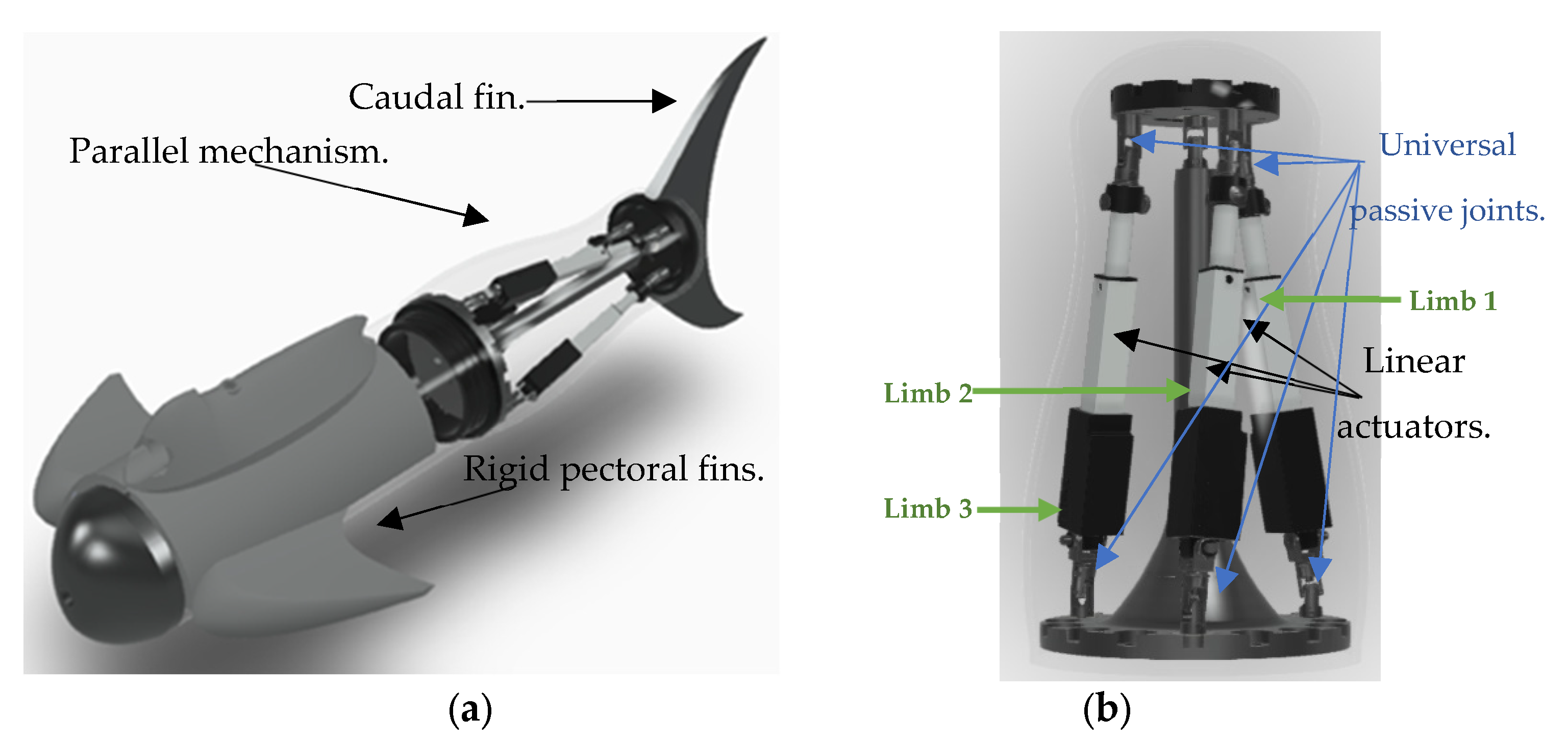
2.1. Propulsion System’s Configuration

The novel propulsion system from the studied BAUV employs a 3 DOF rotational platform with 3UCU-1S limb configuration. Compared to other traditional configurations, the platform was designed for oscillatory motion only. With the oscillation from the platform a caudal fin is moved, producing the propulsion and the thunniform locomotion. The total flapping amplitude for this design ranges from $\pm 30{}^{°}$. Larger flapping amplitudes and higher flapping frequencies result in higher speed and thrust. Figure 1 shows the mechanical design of the propeller and the parallel mechanism that compounds it.

One main feature from this design is its capability to switch between swimming fashions. The moving platform orients the caudal fin according to the desired motion. This allows the vehicle to achieve a vectored thrust and replicate tuna-fish-like or dolphin-like swimming locomotion. From this design, several features should be pointed out:

• The caudal fin is attached to the moving platform. Thrust to the vehicle will be generated by the water displacement produced by the caudal fin. Hence, proper motion control in the platform’s oscillation and frequency is of great interest.
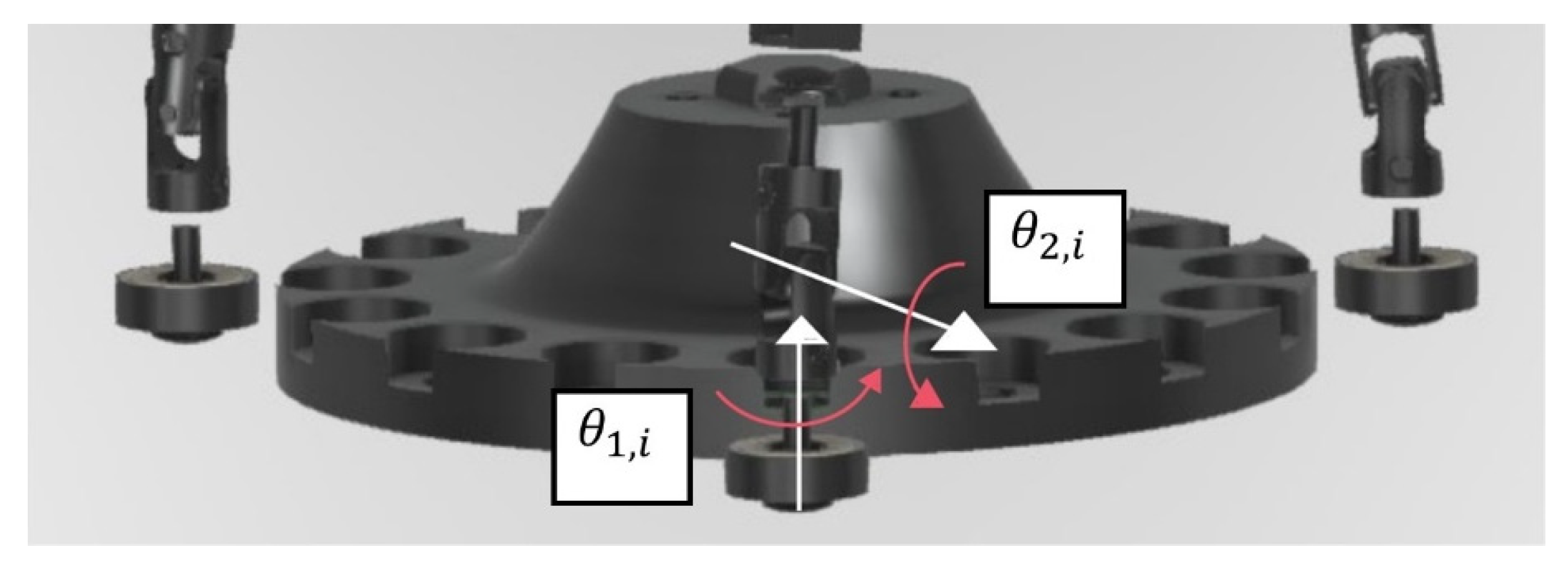
• Three limbs are responsible for moving the platform. The parallel mechanism contains three robotic arms with the same configuration. Each limb contains four passive (non-actuated) universal joints at the beginning and at the end where platforms are attached. One linear (prismatic) actuator is placed between such passive joints and is the responsible of the motion generation for each limb.
• The first limb always acts as a pivot. This configuration is helpful when controlling the flapping motion from the platform. This means that the oscillation from the moving platform will be caused by moving only limbs 2 and 3.
• No translational motion is desired. The incorporation of a fourth restrictive limb with spherical joint at its end links the origins of both platforms. This causes distance from both origins to always stay constant.
• The rotational motion of the platform is analyzed based on the Euler angles disposition and measured respect to an inertial frame fixed on the origin of the fixed platform. Considering that only limbs 2 and 3 cause the moving platform’s oscillation, only two rotational motions of roll ($\beta$) and yaw ($\gamma$) are produced. The roll motion is produced over the Y axis and presents a total range from $\pm 30{}^{°}$. Moreover, the yaw motion is produced over the Z axis and it takes values of $0$ for vertical flapping and 90${}^{°}$ for horizontal flapping. Finally, it is desired that rotational motion from the platform could reach flapping frequencies ranging from 0.5 to 5 Hz.

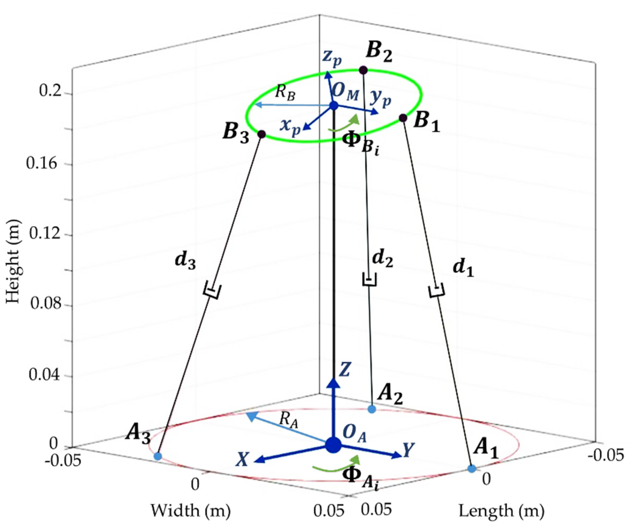
2.2. Propulsion System’s Kinematics Modeling

Kinematics modeling for the moving platform and the limbs system are computed to correctly understand how the propeller can move. The caudal fin’s orientation depends directly on the rotational motion from the platform, and water displacement for thrust generation will depend on its flapping frequency. Since three independent symmetric manipulator arms are responsible of moving the platform, kinematics analysis per limb is detailed as well.

2.2.1. Platform’s Kinematics

Figure 2 describes the free body diagram of the parallel mechanism incorporated inside the propulsion system. The origin of the inertial system $\left\{O_A\right\}$ is positioned at the center of the circular fixed platform of radius $R_A,$ while the moving coordinate system $\left\{O_M\right\}$ finds its origin at the center of the upper platform of radius $R_B$. The moving platform is connected to the limbs by universal joints $B_i,$ which are separated from each other at a certain angle ${\mathsf{\Phi }}_B{}_i.$ Likewise, the other ends of the limbs $A_i$ are connected to the fixed platform by universal joints with an angular separation of ${\mathsf{\Phi }}_A{}_i$. To avoid singularities when switching from swimming fashions, the mechanical design uniformly distributes attachment points $A_i$, while $B_i$ joints are distributed following an uneven configuration [10]. Moreover, three linear actuators vary their length at certain distances $d_i$ to create motion on the mechanism. Hence, by varying the limbs lengths, the upper platform is oriented with respect to the center of the base platform.

The joint positions $\left({}_{B_i}{}^{A}P\right)$ in the moving platform are always measured with respect to the base frame $\left\{O_A\right\}.$ The $X,Y,Z$ coordinate system presents the Z axis pointing upwards and the Y axis pointing to the first universal joint $A_1.$ In the same way, the $x_p,y_p,z_p$ coordinate system presents the $z_p$ axis normal to the moving platform and the $y_p$ axis pointing to the universal joint $B_1.$ Since the relative positions $\left({}_{B_i}{}^{M}P\right)$ of each universal joint with respect to the moving frame are constant for all time, and the position of the origin of the moving frame $\left\{O_M\right\}$ with respect to the fixed frame $\left\{O_A\right\}$ is always constant as well, it will only be necessary to know the orientation of the moving frame $\left\{O_M\right\}$ to compute the position of any universal joint $B_i$ in space. Hence, the location of each universal joint using a homogeneous transformation matrix will be defined by:

$$\left[\begin{array}{c}{}_{B_i}{}^{A}P\\ 1\end{array}\right]=\left[\begin{array}{cc}{}_M{}^{A}R& {}_{O_M}{}^{A}P\\ 0_{\left(1x3\right)}& 1\end{array}\right]\left[\begin{array}{c}{}_{B_i}{}^{M}P\\ 1\end{array}\right], where i=1,23.$$

(1)

From Equation (1), ${}_M{}^{A}R$ is the rotation matrix from $\left\{M\right\}$ with respect to the fixed frame $\left\{A\right\}$. In the present analysis, the platform’s orientation is represented by the pitch-roll-yaw Euler angles:

$${}_M{}^{A}R=R_Z\left(\gamma \right)R_Y\left(\beta \right)R_X\left(\alpha \right)=\left[\begin{array}{ccc}c\beta c\gamma & s\alpha s\beta c\gamma -c\alpha s\gamma & c\alpha s\beta c\gamma +s\alpha s\gamma \\ c\beta s\gamma & s\alpha s\beta s\gamma +c\alpha c\gamma & c\alpha s\beta s\gamma -s\alpha c\gamma \\ -s\beta & s\alpha c\beta & c\alpha c\beta \end{array}\right],$$

(2)

where $s\alpha$ is short notation for sin ($\alpha )$, $c\beta$ is short notation for cos $\left(\beta \right),$ and so on. Additionally, the position vector ${}_{O_M}{}^{A}P$ denotes the constant distance between the origins of both coordinate systems ${\left(P_X, P_Y, P_Z\right)}^T$. Finally, the relative positions ${}_{B_i}{}^{M}P$ of each universal joint respect to the moving frame $\left\{M\right\}$ are defined as:

$${}_{B_1}{}^{M}P=\left[\begin{array}{c}{R}_B\mathrm{c}\left(90\right)\\ R_{B}s\left(90\right)\\ 0\end{array}\right], {}_{B_2}{}^{M}P=\left[\begin{array}{c}{R}_B\mathrm{c}\left(198\right)\\ R_{B}s\left(198\right)\\ 0\end{array}\right], {}_{B_3}{}^{M}P=\left[\begin{array}{c}{R}_B\mathrm{c}\left(342\right)\\ R_{B}s\left(342\right)\\ 0\end{array}\right].$$

(3)

Equations (1) through (3) will be used to determine each universal joint position in space with respect to the fixed coordinate system $\left\{A\right\}.$ Each limb should be controlled to properly attain those spatial positions. Hence, the analysis of the limbs’ configuration and their distribution inside the mechanism should be detailed as well.

Table 1. Parameters and disposition of elements in parallel mechanism.

Parameter	Symbol	Value	Unit
Distance between $\left\{O_A\right\}$ and $\left\{O_M\right\}.$	${}_{O_M}{}^{A}P$	${\left(0, 0, 0.192\right)}^T$	$\mathrm{m}$
Distance from $\left\{O_A\right\}$ to joints $A_i.$1	$R_A$	$0.05$	$\mathrm{m}$
Distance from $\left\{O_M\right\}$ to joints $B_i.$	$R_B$	$0.025$	$\mathrm{m}$
Angular distance between joints $A_i.$	${\mathsf{\Phi }}_{\mathrm{A}}{}_i$	(90, 210, 330)	$\mathrm{deg}$
Angular distance between joints $B_i.$	${\mathsf{\Phi }}_{\mathrm{B}}{}_i$	$\left(90, 198 342\right)$	$\mathrm{deg}$
Roll-pitch-yaw Euler angles.	$\alpha$	$0$	$\mathrm{deg}$
	$\beta$	$\left(-30 \mathrm{to} 30\right)$
	$\gamma$	$\left(0 \mathrm{or} 90\right)$

¹ $i=1,2,3$, for all cases.

specifies the parameters of the parallel mechanism configuration found in Figure 2.

2.2.2. Limbs’ Inverse Kinematics

Each linear actuator $d_i$ should reach spatial positions from each computed universal joint $B_i$ Based on the schematic in Figure 2, each limb length can be computed according to the distance existing between universal joints $\overline{A_i{B}_i}.$ By taking the magnitude of such distance, it is possible to know each limb’s length while the spatial coordinates of $B_i$ change over time. Hence,

$$d_i=\left|\right|\overline{A_i{B}_i}\left|\right|=\left|\right|\overline{O_A{A}_i}+{}_{O_M}{}^{A}P+{}_M{}^{A}R·{}_{B_i}{}^{M}P\left|\right|.$$

(4)

From Equation (4), it is then deduced that desired limbs’ lengths will only depend on the desired orientation from the platform and the value of its roll ($\beta$) and yaw ($\gamma$) motion. Moreover, the kinematics equations of the passive joints could be estimated to facilitate the computation of the reduced inverse dynamics (developed in the next section). Figure 3 shows a closer look at how the rotations are produced inside the designed universal joints. For the further analysis in this article, the joint attaching each linear actuator with its corresponding universal joint is being considered as rigid. Hence, only two rotations $\left({\theta }_{1,i }, {\theta }_{2,i}\right)$ are considered for the inverse kinematic solutions per universal joint. The solution for each revolute motion will depend directly on the spatial position ${}_{B_i}{}^{A}P$ computed to obtain the position of each $B_i$, where ${}_{B_i}{}^{A}P={\left(B_i{}_x, B_i{}_y, B_i{}_z\right)}^T.$

A system of six equations will be employed to estimate each passive joint’s position over time, and they are obtained as follows:

For passive joints attaching limb 1, $\left({\theta }_{1,1 }, {\theta }_{2,1}\right)$ inverse kinematics is defined as:

$${\theta }_{1,1}=atan2\left(B_1{}_x,R_A-B_1{}_y\right) \left(rad\right);$$

(5)

$${\theta }_{2,1}=\frac{\pi }{2}-atan2\left(B_1{}_z,\sqrt{{\left(R_A-B_1{}_y\right)}^2+B_1{}_x^2}\right) \left(rad\right).$$

(6)

where $atan2\left(•Y,•X\right)$ is the two-argument arctangent and $2\pi$ variant of ${\tan }^{-1}\left(\frac{•Y}{•X}\right). X$ and $Y$ subscripts denote the respective components of each ball joint $B_i$ measured from base frame $\left\{O_A\right\}.$ For passive joints attaching limb 2, $\left({\theta }_{1,2 }, {\theta }_{2,2}\right)$ inverse kinematics is defined as:

$${\theta }_{1,2}=\pi +atan2\left(-\left[R_{A}sin\left(\frac{7\pi }{6}\right)-B_2{}_y\right],-\left[R_{A}cos\left(\frac{7\pi }{6}\right)-B_2{}_x\right]\right) \left(rad\right);$$

(7)

$${\theta }_{2,2}=\frac{\pi }{2}-atan2\left(B_2{}_z,\sqrt{{\left(R_{A}cos\left(\frac{7\pi }{6}\right)-B_2{}_x\right)}^2+{\left(R_{A}sin\left(\frac{7\pi }{6}\right)-B_2{}_y\right)}^2}\right) \left(rad\right).$$

(8)

Finally, for the passive joints attaching limb 3, $\left({\theta }_{1,3 }, {\theta }_{2,3}\right)$ are computed as:

$${\theta }_{1,3}=atan2\left(-\left[R_{A}sin\left(\frac{11\pi }{6}\right)-B_3{}_y\right],-\left[R_{A}cos\left(\frac{11\pi }{6}\right)-B_3{}_x\right] \right) \left(rad\right);$$

(9)

$${\theta }_{2,3}=\frac{\pi }{2}-atan2\left(B_3{}_z,\sqrt{{\left(R_{A}cos\left(\frac{11\pi }{6}\right)-B_3{}_x\right)}^2+{\left(R_{A}sin\left(\frac{11\pi }{6}\right)-B_3{}_y\right)}^2} \right) \left(rad\right).$$

(10)

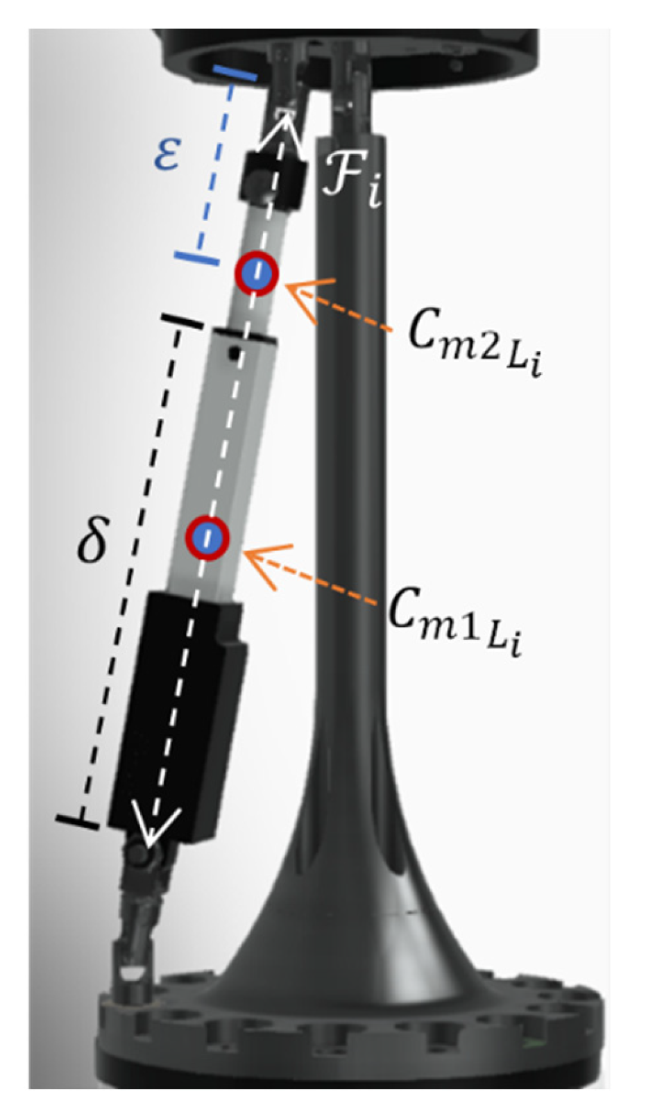
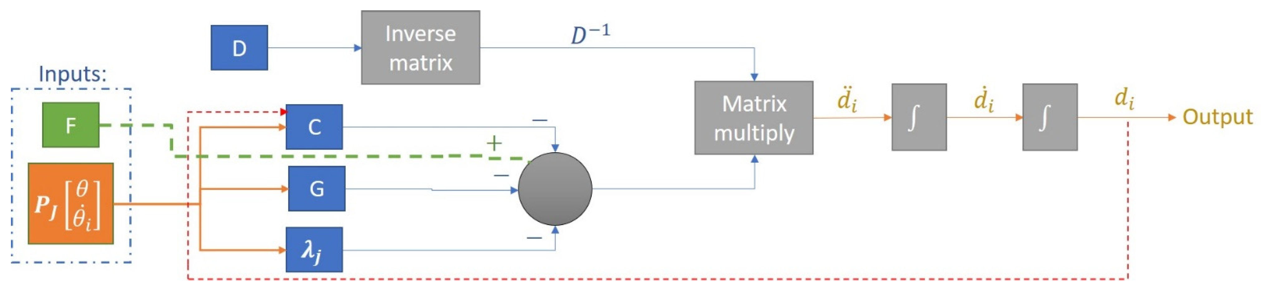
2.3. Propulsion System’s Inverse Dynamic Modeling

The dynamic modeling of parallel manipulators is not straightforward since these systems are based on closed-loop structures. Motion from one limb should be restricted by the other limbs’ motions and the desired pose of the platform. Hence, coupled relationship between system parameters, high nonlinearity in system dynamics and kinematics must be considered [27]. In this article, the reduced inverse dynamic modeling based on the Lagrange formalism was computed. This approach allows one to calculate the actuator forces ${ℱ}_i$ while it deals with the passive joints as a set of equations of closed loop chains. With this analysis, forces applied to the line of action on each actuator can be properly computed to create the desired displacement inside the linear actuators. Figure 4 describes the position of the centers of mass from each actuator and the line of action to which force is applied on each limb.

From Figure 4, the parameter $\delta$ determines the total length from the actuators’ hull to which center of mass $C_{m1}{}_{Li}$ is placed at the middle. Moreover, $\epsilon$ determines the total distance between the attaching point $B_i$ and the center of mass $C_{m2}{}_{Li}$ from the moving piston inside the linear actuator. ${ℱ}_i$ represents the force applied to the actuator and required to generate motion. Hence, the position of each center of mass $({}_{C_{m1}{}_{Li}}{}^{A}P, {}_{C_{m2}{}_{Li}}{}^{A}P)$ inside each limb measured from the inertial frame $\left\{O_A\right\}$ can be defined as:

$${}_{C_{m1}{}_{Li}}{}^{A}P=\left[\begin{array}{c}{R}_{A}c\left({\mathsf{\Phi }}_{\mathrm{A}}{}_i\right)+\left(\raisebox{1ex}{$\delta $}\!\left/ \!\raisebox{-1ex}{$2$}\right.\right)s_{1i}{s}_{2i}\\ R_{A}s\left({\mathsf{\Phi }}_{\mathrm{A}}{}_i\right)-\left(\raisebox{1ex}{$\delta $}\!\left/ \!\raisebox{-1ex}{$2$}\right.\right)c_{1i}{s}_{2i}\\ \left(\raisebox{1ex}{$\delta $}\!\left/ \!\raisebox{-1ex}{$2$}\right.\right)c_{2i}\end{array}\right], {}_{C_{m2}{}_{Li}}{}^{A}P=\left[\begin{array}{c}{R}_{A}c\left({\mathsf{\Phi }}_{\mathrm{A}}{}_i\right)+\left(d_i-\epsilon \right)s_{1i}{s}_{2i}\\ R_{A}s\left({\mathsf{\Phi }}_{\mathrm{A}}{}_i\right)-\left(d_i-\epsilon \right)c_{1i}{s}_{2i}\\ \left(d_i-\epsilon \right)c_{2i}\end{array}\right] for i=1,$$

(11)

$${}_{C_{m1}{}_{Li}}{}^{A}P=\left[\begin{array}{c}{R}_{A}c\left({\mathsf{\Phi }}_{\mathrm{A}}{}_i\right)-\left(\raisebox{1ex}{$\delta $}\!\left/ \!\raisebox{-1ex}{$2$}\right.\right)c_{1i}{s}_{2i}\\ R_{A}s\left({\mathsf{\Phi }}_{\mathrm{A}}{}_i\right)-\left(\raisebox{1ex}{$\delta $}\!\left/ \!\raisebox{-1ex}{$2$}\right.\right)s_{1i}{s}_{2i}\\ \left(\raisebox{1ex}{$\delta $}\!\left/ \!\raisebox{-1ex}{$2$}\right.\right)c_{2i}\end{array}\right], {}_{C_{m2}{}_{Li}}{}^{A}P=\left[\begin{array}{c}{R}_{A}c\left({\mathsf{\Phi }}_{\mathrm{A}}{}_i\right)-\left(d_i-\epsilon \right)c_{1i}{s}_{2i}\\ R_{A}s\left({\mathsf{\Phi }}_{\mathrm{A}}{}_i\right)-\left(d_i-\epsilon \right)s_{1i}{s}_{2i}\\ \left(d_i-\epsilon \right)c_{2i}\end{array}\right] for i=2,$$

(12)

$${}_{C_{m1}{}_{Li}}{}^{A}P=\left[\begin{array}{c}{R}_{A}c\left({\mathsf{\Phi }}_{\mathrm{A}}{}_i\right)+\left(\raisebox{1ex}{$\delta $}\!\left/ \!\raisebox{-1ex}{$2$}\right.\right)c_{1i}{s}_{2i}\\ R_{A}s\left({\mathsf{\Phi }}_{\mathrm{A}}{}_i\right)+\left(\raisebox{1ex}{$\delta $}\!\left/ \!\raisebox{-1ex}{$2$}\right.\right)s_{1i}{s}_{2i}\\ \left(\raisebox{1ex}{$\delta $}\!\left/ \!\raisebox{-1ex}{$2$}\right.\right)c_{2i}\end{array}\right], {}_{C_{m2}{}_{Li}}{}^{A}P=\left[\begin{array}{c}{R}_{A}c\left({\mathsf{\Phi }}_{\mathrm{A}}{}_i\right)+\left(d_i-\epsilon \right)c_{1i}{s}_{2i}\\ R_{A}s\left({\mathsf{\Phi }}_{\mathrm{A}}{}_i\right)+\left(d_i-\epsilon \right)s_{1i}{s}_{2i}\\ \left(d_i-\epsilon \right)c_{2i}\end{array}\right] for i=3.$$

(13)

From Equations (11)–(13), $c_{1i}, c_{2i}, s_{1i}, s_{2i}$ are short notations for $\cos \left({\theta }_{1i}\right),\cos \left({\theta }_{2i}\right),\sin \left({\theta }_{1i}\right), \sin \left({\theta }_{2i}\right)$ respectively. Furthermore, the Lagrange formalism is applied from the concepts of work and energy present on the whole mechanism. The Lagrange equation describes the difference between the kinetic and potential energies ($E_K, E_P$, respectively) from all the moving parts of the system. As previously stated, the parallel mechanism consists of three independent symmetric manipulator arms, whose centers of mass are placed on the same position for each actuator. Additionally, for the present study, it is assumed that the friction forces at all joints are negligible. The total kinetic energy of the whole system is defined as:

$$E_K=E_{K_P}+{\displaystyle \sum }_{i=1}^3{E}_{K_{Li}},$$

(14)

where $E_{K_P}$ is the kinetic energy from the platform and $E_{K_{Li}}$ is the kinetic energy from limb $i.$ Since the platform only presents rotational motion, the equation of kinetic energy $E_{K_P}$ is defined as:

$$E_{K_P}=\frac{1}{2}{I}_P\left({\dot{\alpha }}^2+{\dot{\beta }}^2+{\dot{\gamma }}^2\right),$$

(15)

where $I_P$ is the inertial moment computed for the solid disk that compounds the moving platform and $\omega ={\left(\dot{\alpha },\dot{\beta },\dot{\gamma }\right)}^T$ is the angular velocity of the platform. The center of mass on the moving platform is placed at the origin of the reference frame $\left\{O_M\right\}.$ On the other hand, the equation of kinetic energy on each limb $i$ will consequently be defined as:

$$\begin{gathered} E_{K_{Li}}=\frac{1}{2}{\left({\dot{\theta }}_{1,i}\right)}^2\left[m_1{\left(\raisebox{1ex}{$\delta $}\!\left/ \!\raisebox{-1ex}{$2$}\right.\right)}^2{\left(s_{2i}\right)}^2+I_L+m_2{\left(d_i-\epsilon \right)}^2{\left(s_{2i}\right)}^2+I_U\right] \\ +\frac{1}{2}{\left({\dot{\theta }}_{2,i}\right)}^2\left[m_1{\left(\raisebox{1ex}{$\delta $}\!\left/ \!\raisebox{-1ex}{$2$}\right.\right)}^2+I_L+m_2{\left(d_i-\epsilon \right)}^2+I_U\right]+\frac{1}{2}{\left({\dot{d}}_i\right)}^2{m}_2. \end{gathered}$$

(16)

In Equation (16), $I_L$ represents the inertial moment from the first part of the limb (actuator’s hull) while $I_U$ represents the inertial moment of the upper part of the actuator. Furthermore, the potential energy for the whole system will be defined as:

$$E_P=E_{P_P}+{\displaystyle \sum }_{i=1}^3{E}_{P_{Li}}.$$

(17)

Since the parallel mechanism is designed to only follow rotational motions, the potential energy at the moving platform $E_{P_P}$ at its center of mass will not vary over time. It will be defined as:

$$E_{P_P}=M_{P}g{}_{O_M}{}^{A}P;$$

(18)

where $M_P$ is the mass of the moving platform, $g$ is the gravitational acceleration and ${}_{O_M}{}^{A}P$ is the height presented between platforms. The potential energy at the centers of mass from each limb $i$ is defined as:

$$E_{P_{Li}}=m_{1}g\left[\left(\raisebox{1ex}{$\delta $}\!\left/ \!\raisebox{-1ex}{$2$}\right.\right)c_{2i}\right]+m_{2}g\left[\left(d_i-\epsilon \right)c_{2i}\right].$$

(19)

Finally, using Equations (14)‒(19), the Lagrange equation $ℒ$ for the whole system is defined as:

$$ℒ=E_K-E_P.$$

(20)

Derivation of Limb’s Force Equations

Actuating forces ${ℱ}_1, {ℱ}_2, {ℱ}_3$ applied to the limbs are to be found based on the derivation of the Lagrange equation from the previous analysis. For the present design, the normalized limb lengths $d_i$ are the independent generalized coordinates and the revolute ${\theta }_{1,i}, {\theta }_{2,i}$ inside the universal passive joints are the dependent generalized coordinates. Then, the Lagrange equations of motion are defined by:

$$\frac{d}{dt}\left(\frac{\partial ℒ}{\partial q_j}\right)-\left(\frac{\partial ℒ}{\partial q_j}\right)+{\displaystyle \sum }_{k=1}^6{\lambda }_k \frac{\partial f_k}{\partial q_j}={\mathbb{Q}}_j; j=1,\dots ,9,$$

(21)

where:

$$q_j=\{\begin{array}{cc}{d}_i& j=i=1,2,3\\ {\theta }_{1,i}& j=4,5,6;i=1,2,3\\ {\theta }_{2,i}& j=7,8,9;i=1,2,3\end{array} \mathrm{and} {\mathbb{Q}}_j=\{\begin{array}{cc}{ℱ}_i& j=i=1,2,3\\ 0& j=4,\dots ,9\end{array}.$$

In real-time applications when controlling these types of mechanisms, the platform’s orientation, velocity, and acceleration are known or predetermined. It is based on such predispositions where the interest of determining the forces required to actuate the limbs is of paramount importance. By properly defining the force necessary to actuate the links, the platform will follow a desired trajectory. Equation (21) defines a system of 9 equations to which the first three serve the purpose of computing the values of the forces applied on each actuator (when $j=1,2,3$). Additionally, to correctly solve the system, six constraint equations $f_k$ that are functions of $d_i, {\theta }_{1,i}, {\theta }_{2,i}$, and their time derivatives, should be properly defined. Moreover, the six Lagrange multipliers ${\lambda }_k$ should be solved by solving iteratively six simultaneous equations, i.e., Equation (21) when $j=4,\dots 9.$

Based on the schematic of the kinematics chains from Figure 2, two vectorial closed loop constraint equations may be defined as follows:

$$\overrightarrow{\left\{O_A\right\}{A}_1}+\overrightarrow{A_1{B}_1}+\overrightarrow{B_1\left\{O_M\right\}}+\overrightarrow{\left\{O_M\right\}{B}_2}+\overrightarrow{B_2{A}_2}+\overrightarrow{A_2\left\{O_B\right\}}=0,$$

(22)

$$\overrightarrow{\left\{O_A\right\}{A}_2}+\overrightarrow{A_2{B}_2}+\overrightarrow{B_2\left\{O_M\right\}}+\overrightarrow{\left\{O_M\right\}{B}_3}+\overrightarrow{B_3{A}_3}+\overrightarrow{A_3\left\{O_B\right\}}=0.$$

(23)

Vectorial Equations (22) and (23) are rewritten as scalar equations to generate the six constraint equations $f_k$ where $\left(k=1,\dots ,6\right)$:

$$R_{A}c\left({\mathsf{\Phi }}_{\mathrm{A}}{}_1\right)+d_1{s}_{11}{s}_{21}+d_2{c}_{12}{s}_{22}-R_{A}c\left({\mathsf{\Phi }}_{\mathrm{A}}{}_2\right)-{}_M{}^{A}R{}_{B_1}{}^{M}P{}_x+{}_M{}^{A}R{}_{B_2}{}^{M}P{}_x=0;$$

(24)

$$R_{A}s\left({\mathsf{\Phi }}_{\mathrm{A}}{}_1\right)-d_1{c}_{11}{s}_{21}-{}_M{}^{A}R{}_{B_1}{}^{M}P{}_y+{}_M{}^{A}R{}_{B_2}{}^{M}P{}_y+d_2{s}_{12}{s}_{22}-R_{A}s\left({\mathsf{\Phi }}_{\mathrm{A}}{}_2\right)=0;$$

(25)

$$d_1{c}_{21}-d_2{c}_{22}-{}_M{}^{A}R{}_{B_1}{}^{M}P{}_z+{}_M{}^{A}R{}_{B_2}{}^{M}P{}_z=0;$$

(26)

$$R_{A}c\left({\mathsf{\Phi }}_{\mathrm{A}}{}_2\right)-d_2{c}_{12}{s}_{22}-{}_M{}^{A}R{}_{B_2}{}^{M}P{}_x+{}_M{}^{A}R{}_{B_3}{}^{M}P{}_x-d_3{c}_{13}{s}_{23}-R_{A}c\left({\mathsf{\Phi }}_{\mathrm{A}}{}_3\right)=0;$$

(27)

$$R_{A}s\left({\mathsf{\Phi }}_{\mathrm{A}}{}_2\right)-d_2{s}_{12}{s}_{22}-{}_M{}^{A}R{}_{B_2}{}^{M}P{}_y+{}_M{}^{A}R{}_{B_3}{}^{M}P{}_y-d_3{s}_{13}{s}_{23}-R_{A}s\left({\mathsf{\Phi }}_{\mathrm{A}}{}_3\right)=0;$$

(28)

$$d_2{c}_{22}-d_3{c}_{23}-{}_M{}^{A}R{}_{B_2}{}^{M}P{}_z+{}_M{}^{A}R{}_{B_3}{}^{M}P{}_z=0.$$

(29)

Finally, the actuating force along the $i$th limb is computed by directly solving Equation (21), using the computation of $ℒ$ and $f_k$ and its derivatives with respect to $d_i$. The three equations of force required per limb on the designed system are then defined as:

$$\begin{gathered} {ℱ}_1=\ddot{d_1}{m}_2-{\left({\dot{\theta }}_{1,1}\right)}^2{m}_2\left(d_1-\epsilon \right){\left(s_{21}\right)}^2-{\left({\dot{\theta }}_{2,1}\right)}^2{m}_2\left(d_1-\epsilon \right)+m_{2}g{c}_{21} \\ -{\lambda }_1{s}_{11}{s}_{21}+{\lambda }_2{c}_{11}{s}_{21}-{\lambda }_3{c}_{21}; \end{gathered}$$

(30)

$$\begin{gathered} {ℱ}_2=\ddot{d_2}{m}_2-{\left({\dot{\theta }}_{1,2}\right)}^2{m}_2\left(d_2-\epsilon \right){\left(s_{22}\right)}^2-{\left({\dot{\theta }}_{2,2}\right)}^2{m}_2\left(d_2-\epsilon \right)+m_{2}g{c}_{22} \\ -{\lambda }_1{c}_{12}{s}_{22}-{\lambda }_2{s}_{12}{s}_{22}+{\lambda }_3{c}_{22}+{\lambda }_4{c}_{12}{s}_{22}+{\lambda }_5{s}_{12}{s}_{22}-{\lambda }_6{c}_{22}; \end{gathered}$$

(31)

$$\begin{gathered} {ℱ}_3=\ddot{d_3}{m}_2-{\left({\dot{\theta }}_{1,3}\right)}^2{m}_2\left(d_3-\epsilon \right){\left(s_{23}\right)}^2-{\left({\dot{\theta }}_{2,3}\right)}^2{m}_2\left(d_3-\epsilon \right)+m_{2}g{c}_{23} \\ +{\lambda }_4{c}_{13}{s}_{23}+{\lambda }_5{s}_{13}{s}_{23}+{\lambda }_6{c}_{23}. \end{gathered}$$

(32)

Equations (30)‒(32) might be rearranged so that the robotic system can be defined by a dynamic equation in matrix form. Hence, the forces required to actuate each limb will be defined as:

$$F_i=D{\ddot{d}}_i+C\left(d,\theta ,{\dot{\theta }}_i\right){\theta }_{\left(1,2\right),i}+G{\theta }_{2,i}+{\lambda }_j;$$

(33)

where $F_i$ is the (3 × 1) matrix containing the required forces ${\left({ℱ}_1,{ℱ}_2,{ℱ}_3\right)}^T$, $D$ is a (3 × 3) diagonal mass matrix, $C$ is a (3 × 6) Coriolis and centrifugal forces matrix, $G$ is the (3 × 1) gravitational forces matrix, and ${\lambda }_j$ is the (3 × 1) Lagrange multipliers and constraints matrix. By making some manipulation over Equation (33), the final plant to which control strategies are being implemented will be defined as:

$${\ddot{d}}_i=D^{-1}\left[F_i-C\left(d,\theta ,{\dot{\theta }}_i\right){\theta }_{\left(1,2\right),i}-G{\theta }_{2,i}-{\lambda }_j\right].$$

(34)

Figure 5 shows the block diagram of the plant and describes how Equation (34) will be iteratively computed on simulations. As explained throughout the last two sections, the plant will require two main inputs: the forces previously computed by a controller and the estimated values from the passive joints. The plant’s output will show the real limb’s position over time and will be compared to desired limb’s length according to the trajectory defined for the moving platform.

2.4. Path Tracking and Control

2.4.1. Feedback PD Controller

The moving platform is set to follow a desired trajectory over time. The platform changes its orientation by making a roll motion $\left(\beta \right)$ over the $Y$ axis. As previously stated, the pitch $\left(\alpha \right)$ and yaw $\left(\gamma \right)$ motions stay constant through all time. By changing the speed at which the platform changes its orientation, different thrust and water displacement will be produced. Since the caudal fin attached to the moving platform is the only propulsion system for the designed vehicle, attaining a precise control over limbs displacements will be important to achieve the desired motion. Higher flapping frequencies will demand greater control actions and will produce higher thrust levels. Figure 6 describes the block diagram of a closed-loop PD control system where the limb distance $d_i$ is regulated based on the change of the desired platform’s orientation $\beta$ through time $t$.

The desired trajectory (orientation) that the platform is set to follow based on pitch-roll-yaw angles through time will be set as:

$$f\left(\alpha ,\beta ,\gamma ,t\right)=\{\begin{array}{c}\begin{array}{cc}\alpha =0,& t\ge 0\end{array}\\ \begin{array}{cc}\beta =30\ast \sin \left(2\pi ft\right),& t\ge 0\end{array}\\ \begin{array}{cc}\gamma =0, & t\ge 0\end{array}\end{array}.$$

(35)

The flapping frequencies $f$ to which the caudal fin is set to oscillate will range from 0.5 to 5 Hz. The total amplitude of oscillation (by design) is set to $\pm 30{}^{°}.$ Moreover, the control law for the implemented PD is defined as:

$$F_i\left(t\right)=kp·e_i\left(t\right)+kd·\dot{e_i}\left(t\right)\hspace{1em}\hspace{1em},i=1,2,3;$$

(36)

where:

$$e_i\left(t\right)=d_i{}_D\left(t\right)-d_i{}_R\left(t\right),$$

(37)

$$\dot{e_i}\left(t\right)=\frac{e_i\left(t\right)-e_i\left(t-1\right)}{\mathsf{\Delta }t}.$$

(38)

The proportional and derivative gains for the PD controller are arbitrary defined to attain critical damping. Hence, the relation between $kp$ and $kd$ is established by the following relation:

$$kd=2\sqrt{kp}.$$

(39)

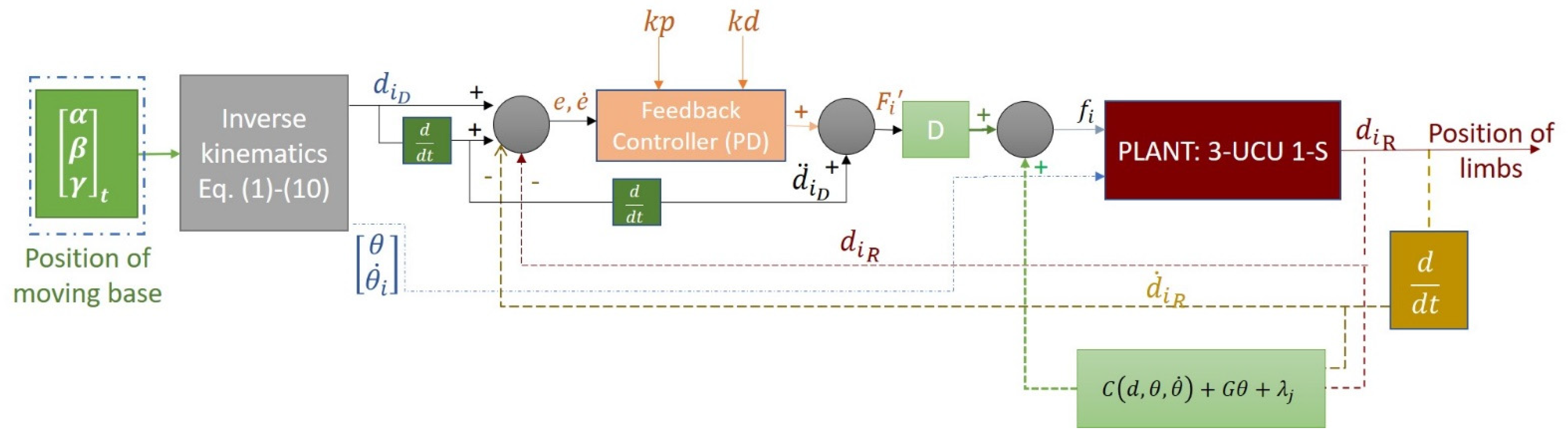
2.4.2. Feedforward Plus Feedback Controller

The second control strategy applied intends to attain greater levels of precision when following trajectories. Feedforward controllers consider using the model of the robot’s dynamics to proactively generate forces instead of waiting for errors. Inside this strategy, the controller computes the control action based on the desired position, velocity, and acceleration from the trajectory generator, and the system’s dynamics [28]. In real applications, platform’s dynamic analysis will not always exactly represent real-life circumstances. Moreover, some non-considered disturbances from environment dynamics and inside the mechanism may cause unwanted reactions. Because of this, adding the feedback term (such as the PD controller detailed on the previous section) will deal with all non-considered robot and environment dynamics. Hence, using a feedforward controller based on the dynamic analysis from the studied plant and adding the previous PD term should result in an improved performance for the path tracking problem faced by each limb. Additionally, the proper choice of gains $\left(kp, kd\right)$ will ensure exponential decay of the trajectory error. In order to make a fair comparison between these first two control strategies, proportional and derivative gains from the feedback and the feedforward plus feedback controllers will remain constant.

Remembering that (33) presents the dynamic equation for the forces $F_i$ required to actuate each limb, the new control law for the force entering the plant will be reformulated as:

$$f_i=\propto F_i^{\prime }+\mathsf{H};$$

(40)

where $\propto$ is the diagonal mass matrix $D, \mathsf{H}$ is the sum of the Coriolis, gravitational and Lagrange constraint matrices, and $F_i^{\prime }$ is the law control from the PD controller. By expanding and solving for Equations (33) and (40), the feedback control output $F_i^{\prime }$ will be defined as:

$$\begin{gathered} D{\ddot{d}}_i+C\left(d,\theta ,{\dot{\theta }}_i\right){\theta }_{\left(1,2\right),i}+G{\theta }_{2,i}+{\lambda }_j= D{F}_i^{\text{'}}+C\left(d,\theta ,{\dot{\theta }}_i\right){\theta }_{\left(1,2\right),i}+G{\theta }_{2,i}+ {\lambda }_j\therefore \\ {F}_i^{\text{'}}={\ddot{d}}_i. \end{gathered}$$

(41)

Moreover, to achieve the linear error dynamics, the desired acceleration on limbs ${\ddot{d_i}}_D$ should be computed and the feedback of $d_i$ and $\dot{d_i}$ should be employed to compute position and velocity errors $e$ and $\dot{e}.$ Then, by working on (41), the control action from the PD feedback controller will be defined as:

$${\ddot{d}}_i={\ddot{d}}_i{}_D+kp·e_i\left(t\right)+kd·\dot{e_i}\left(t\right)\hspace{1em}\hspace{1em}\mathrm{for} i=1,2,3.$$

(42)

With the implementation of a feedforward plus feedback controller, it is desired to find a closed loop control where the dynamic behavior of the system is anticipated. This controller should be able to compensate for the dynamics of the system in the presence of perturbations and abrupt changes by working with the accelerations attained inside the whole model. Then, by complementing actions with help of the classic PD controller, error is intended to decay while achieving a smooth performance for the forces applied to the plant. Figure 7 describes the block diagram for the implementation of the feedforward plus feedback controller.

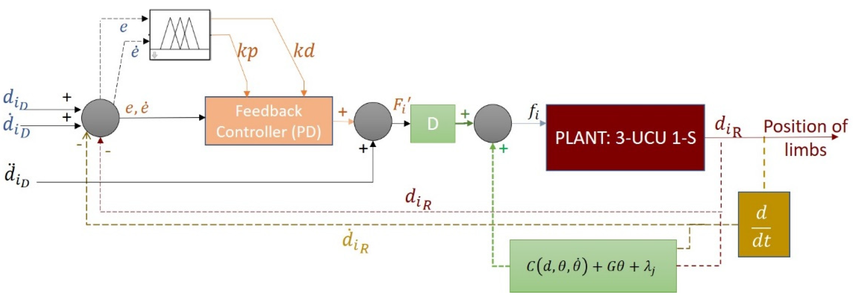
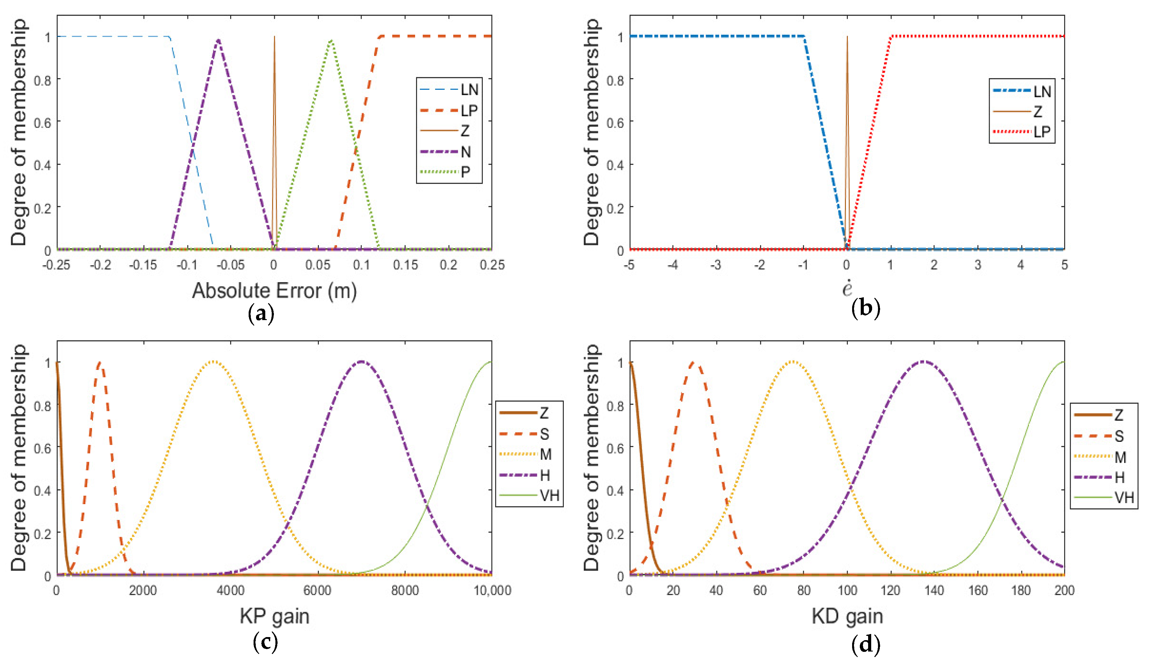
2.4.3. Adaptive Fuzzy Feedback Controller

When using classic feedback controllers (as a PD) to solve the path tracking problem, the proper tuning of gains will be of great help to accurately reduce error levels when attaining desired trajectories. Furthermore, when using more precise control systems such as a feedforward plus feedback controller, adapting gains could guarantee a better performance and a greater error reduction. This article also details the design of a Fuzzy logic system able to determine which of the gains $kp$ or $kd$ would work better during the feedback phase inside the previous control strategies. Based on the error’s behavior and its time derivative, the fuzzy controller iteratively defines values for the PD’s gains in order to reduce the error rate. Since the goal is to attain high rotation speeds from the moving platform (up to 5 Hz), the control task gets more difficult. At higher flapping frequencies, sudden changes when following preestablished trajectories tend to occur. Hence, an adaptable controller that can adjust based on the change of error will be helpful when computing the limbs acting forces. Figure 8 describes the block diagram of the gain channeling fuzzy logic controller as a previous step for tuning the PD gains inside the feedforward plus feedback control strategy. The Fuzzy logic system for gain tuning was also implemented for the plain feedback controller described in Figure 6.

Fuzzy logic controllers (FLC) are known for providing human reasoning inside the decision making in the format of rules. The designed FLC is of Mamdani-type. This means that the process of adjusting $kp$ and $kd$ gains will consist of a three-part process: fuzzification, rule-based reasoning, and defuzzification [29]. As seen in Figure 8, the designed Fuzzy-PD controller takes the computations of limbs positional error $e$ and its derivate $\dot{e}$ as inputs and decides to assign coefficients for $kp$ and $kd$ (system’s output) according to a “if–then” set of rules. This means that the PD controller’s gains will be iteratively updated based on the error’s behavior from each limb when following the desired path.

For the fuzzification stage, crisp input values of $e$ and $\dot{e}$ are processed by triangle and trapezoid membership functions (MFs). The linguistic terms for $e$ are large negative (LN), negative (N), zero (Z), Positive (P) and large positive (LP), where (LN) and (LP) present trapezoid MFs and (N), (Z) and (P) present triangle MFs. On the other hand, only three linguistic terms are defined for $\dot{e}:$ negative (N), zero (Z) and positive (P), where (Z) is a triangle and the other two trapezoid MFs. Two output variables were defined for the defuzzification process: KP and KD. For the defuzzification stage, all linguistic terms for the output variables present gaussian MFs. Even though both output variables are computed separately, they present the same linguistic terms: zero (Z), small (S), medium (M), high (H) and very high (VH). Figure 9 shows the membership functions and the linguistic terms for the inputs and outputs from each FLC. Three FLCs are implemented to compute the $k{p}_i$ and $k{d}_i$, respectively, based on each limb’s $e_i\left(t\right)$ and ${\dot{e}}_i\left(t\right)$.

Table 2. Fuzzy control rules for $k{p}_i$ and $k{d}_i$.

$\mathit{k}{\mathit{p}}_{\mathit{i}}$$/\mathit{k}{\mathit{d}}_{\mathit{i}}$		${\mathit{e}}_{\mathit{i}}$
		LN	N	Z	P	LP
${\dot{\mathit{e}}}_{\mathit{i}}$	N	VH/VH	H/H	S/M	H/H	VH/VH
	Z	VH/VH	M/M	Z/Z	M/M	VH/VH
	P	VH/VH	H/H	S/M	H/H	VH/VH

shows the 15 rules for the inference stage, where inputs’ linguistic terms are associated with outputs’ linguistic terms based on an if–then structure. The fuzzy rules follow the Mamdani’s max-min method, and at the defuzzification stage, the crisp output signal is computed by using the centroid method.

2.5. Simulations

The propulsion system was simulated using Simulink from MatLab^®. During simulations, the reduced inverse dynamics developed in the present article were considered as the plant. The platform was set to follow a rotation over the $Y$ axis with roll, pitch and yaw motions defined in (35). From such motions, universal upper joints $B_i$ were computed as well as desired limb lengths. The controlled variable was then the required force ${ℱ}_i$ to actuate the limbs so that upper joints might be reached. Four controllers were implemented for such task: PD, Fuzzy-PD (FUPD), Feedforward Plus PD (FFPD), and Feedforward Plus Fuzzy-PD (FFUPD). Each simulation consisted of the generation of the flapping trajectory over a period of 5 s. For all cases, the flapping total amplitude was set to $\pm 30{}^{°}$. Moreover, the flapping frequency was increased during simulations from 0.5 to 5 Hz, with steps of 0.5 Hz. The simulations’ purpose was of visualizing which controllers could effectively handle the path tracking problem while frequency increased (since high frequencies are desired for thrust generation inside BAUVs). Each controller was responsible for computing the required acting force from each limb separately. Additionally, the same set of fuzzy rules, and input and output variables, were employed for the implementation of the FUPD and FFUPD controllers. Finally, simulations followed the parameters from

Table 3. Parameters for the implementation of simulations.

Parameter	Symbol	Value	Unit
Actuator’s hull length.	$\delta$	0.068	$\mathrm{m}$
Distance from joint $B_i$ to $C{m}_2{}_{Li}.$	$\epsilon$	0.025	$\mathrm{m}$
Mass of actuator’s hull.	$m_1$	0.054	$\mathrm{kg}$
Mass of actuator’s piston.	$m_2$	0.250	$\mathrm{kg}$
Platform’s moment of inertia.	$I_P$	1.09$\times {10}^{-4}$	$\mathrm{kg}·{\mathrm{m}}^2$
Actuator’s hull inertial moment.	$I_L$	3.8 $\times {10}^{-6}$	$\mathrm{kg}·{\mathrm{m}}^2$
Actuator’s piston inertial moment.	$I_U$	4.5 $\times {10}^{-6}$	$\mathrm{kg}·{\mathrm{m}}^2$
Gravitational acceleration.	$g$	9.81	$\mathrm{m}·{\mathrm{s}}^{-2}$
Proportional PD gain.	$kp$	2500	-
Derivative PD gain.	$kd$	100	-

.

Two set of simulations were conducted:

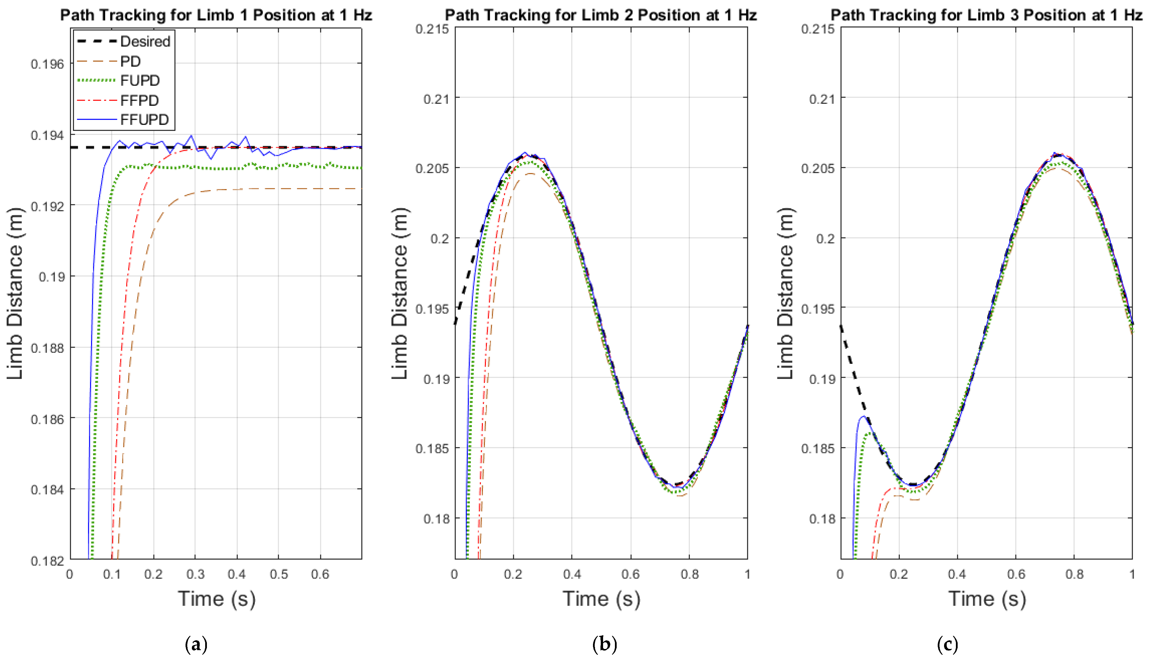
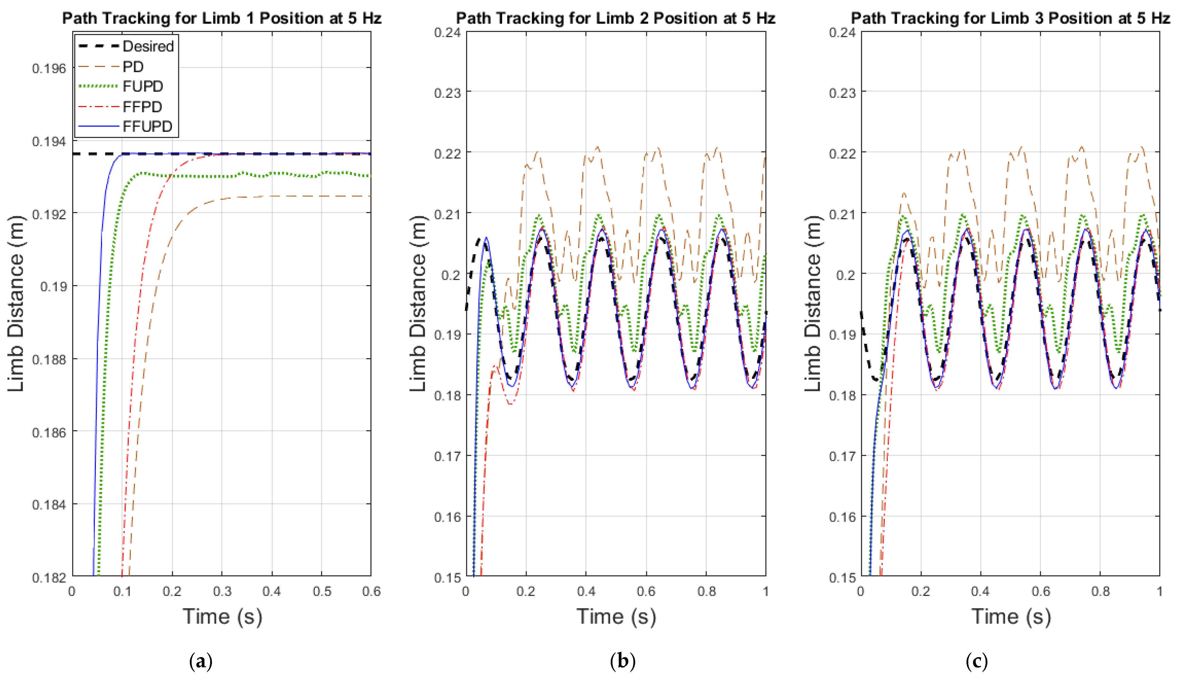
• Set 1 of simulations: The effectiveness of four controllers was tested based on the comparison of how each limb could reach the desired length when the platform changed its position over time. The precision of following the desired trajectory for each limb was compared for the whole spectrum of flapping frequencies.
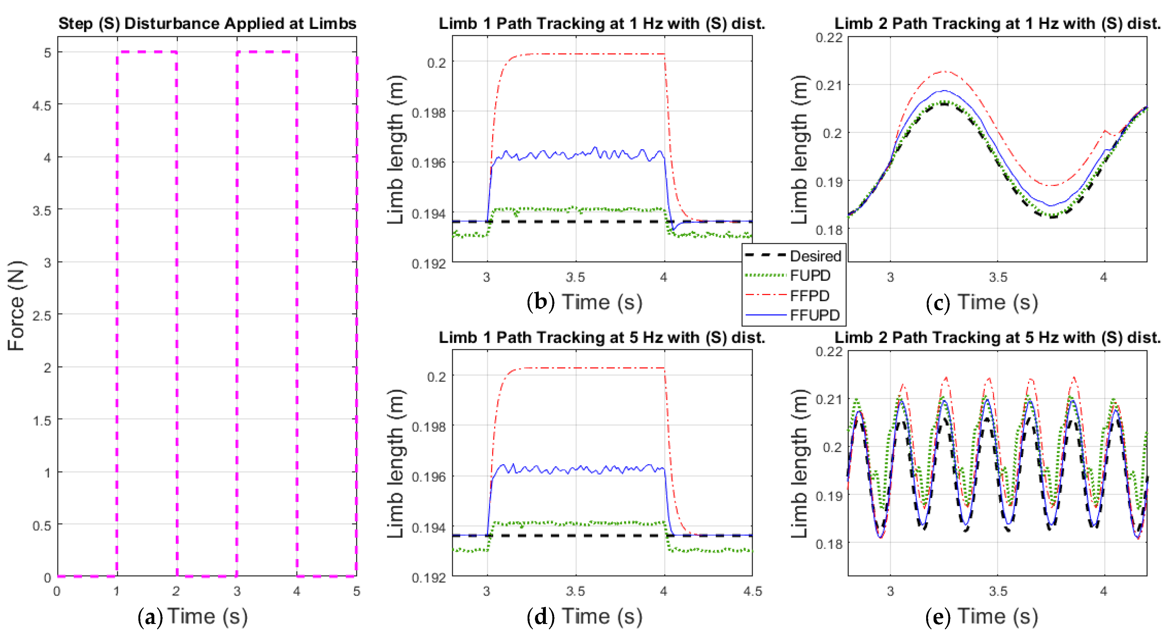
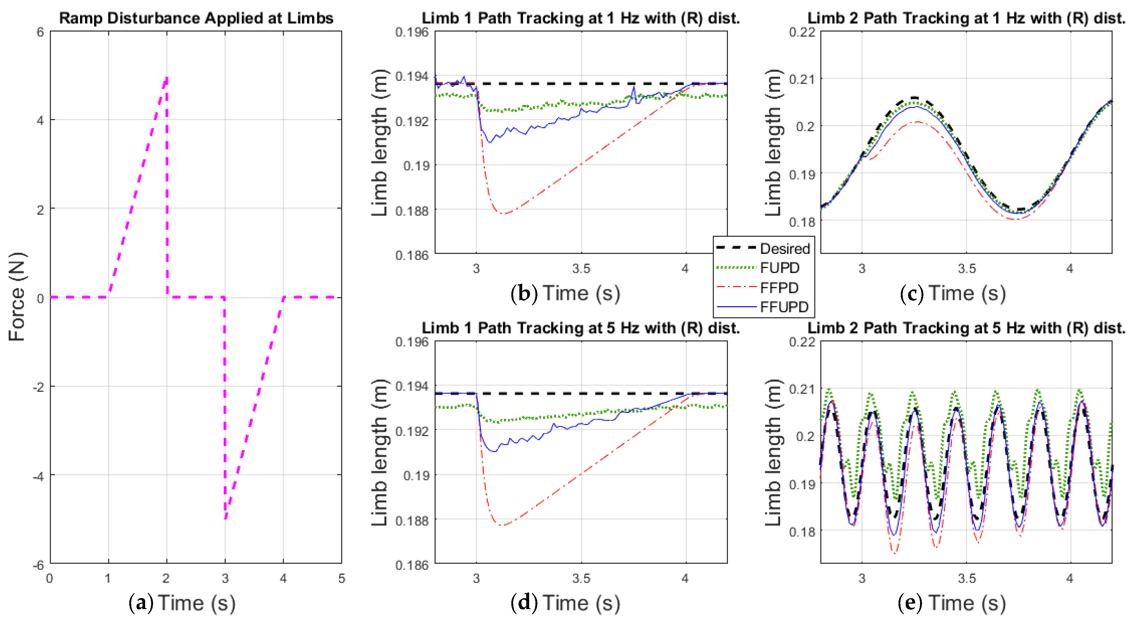
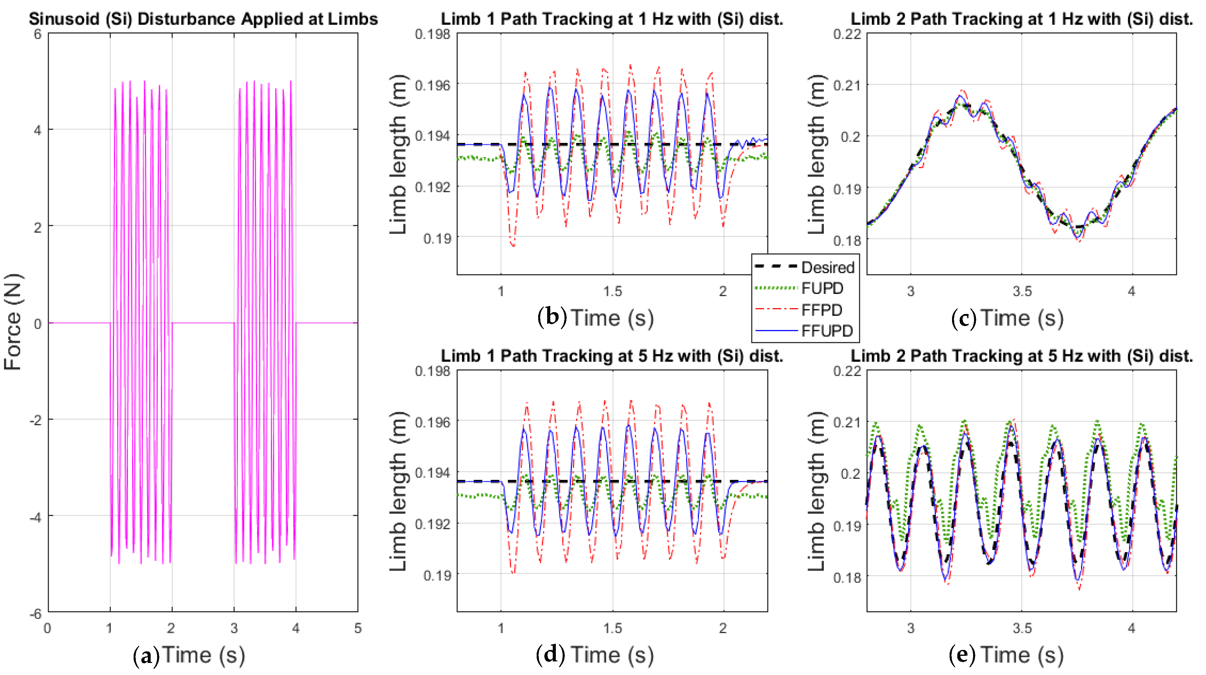
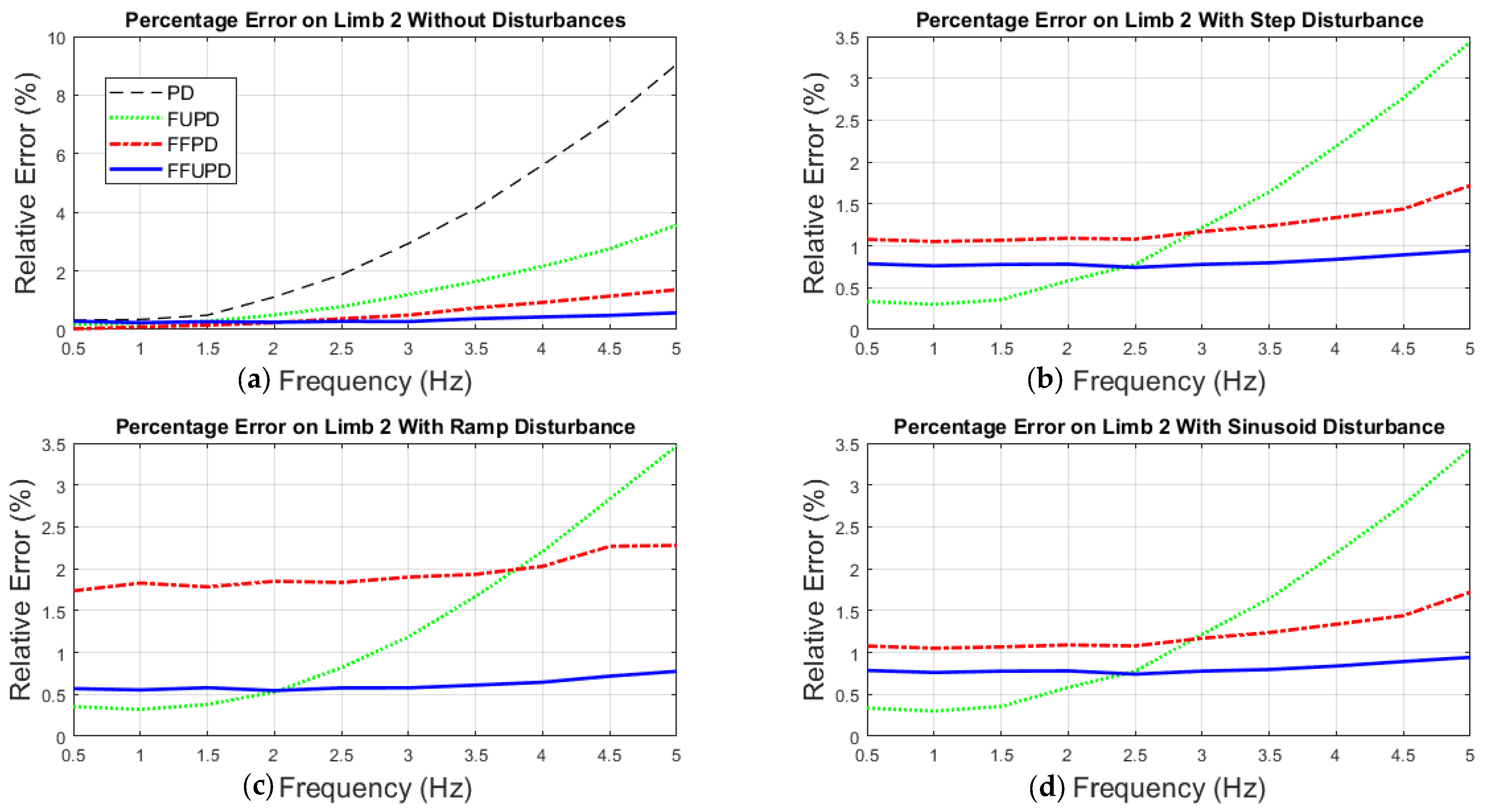
• Set 2 of simulations: The desired platform’s trajectory and flapping frequencies stayed constant as the previous set, but disturbances were added to each limb’s line of action. Three different types of disturbances were simulated and added to the plant: step (S), ramp (R) and sinusoid (Si), mathematically defined by:

$$f\left(S,t\right)=\{\begin{array}{cc}0,& 0\le t<1; 2\le t<3;t\ge 4\\ 5,& 1\le t<2; 3\le t<4\end{array} \left(N\right),$$

(43)

$$f\left(R,t\right)=\{\begin{array}{cc}0,& 0\le t<1; 2\le t<3;t\ge 4;\\ 5\left(t-1\right),& 1\le t<2;\\ 5\left(t-4\right),& 3\le t<4\end{array} \left(N\right),$$

(44)

$$f\left(Si,t\right)=\{\begin{array}{cc}0,& 0\le t<1; 2\le t<3;t\ge 4\\ 5\sin \left(17\pi t\right),& 1\le t<2; 3\le t<4\end{array}\left(N\right).$$

(45)

During each simulation, the percentage relative error $E_{rel\left(i\right)}$ was iteratively computed during the steady state for set 1 and during the presence of disturbances for set 2. To better compare the effectiveness from each controller in the path tracking task, the RMS average of $E_{rel\left(i\right)}$ was computed at the end of each simulation. Then:

$$E_{rel\left(i\right)}\left(t\right)=\frac{e_i\left(t\right)}{d_i{}_D\left(t\right)}\times 100 (\%);$$

(46)

3. Results and Discussion

Figure 10 and Figure 11 show the results from set 1 of simulations. While Figure 10 describes the path tracking problem for the three limbs at 1 Hz, the latter does it at 5 Hz. Without a proper control, limbs will fail at attaining desired positions once the flapping frequency starts to increase, which can be visualized by comparing results from both figures. The three limbs could have followed their assigned trajectories when the flapping frequencies were as low as 1 Hz. However, once the flapping frequency of the moving platform increased to 5 Hz, abrupt changes of position could not be correctly overcome by the classic PD controller or the adaptive FUPD controller. The feedforward stage from the FFPD and FFUPD controllers better adapted and reacted to sudden changes and presented better performances while frequency increased. Since limb 1 was assigned as a pivot and did not suffer of abrupt changes, any of the four employed controllers could have served for the task of keeping it in position. However, as seen on Figure 10a and Figure 11a, PD and FUPD present a steady-state error. Since adaptive controllers (FUPD, FFUPD) are iteratively tuning the proportional and derivative gains, they present faster responses when overcoming the initial state error inside all examples. Moreover, it is visualized how limb 2 and 3 move in a synchronized way, hence, for further analysis (and for reasons of brevity) it would only be necessary to focus on the behavior of one of them.

Figure 12 presents the control action taken by the adaptive FUPD, FFUPD and the FFPD controllers. The shown graphs from the first row are the required forces for limb 1 to keep position when the platform is flapping at 1 Hz (a through c). The second row of graphs details the required forces to make limb 2 follow a desired trajectory when the platform is flapping at 1 Hz as well (d through f). The final row describes the required forces to move limb 2 when the platform is flapping at 5 Hz (g through h). Since the FUPD controller iteratively adapts according to the error’s behavior and its changing rate, shattering is produced on the action of control, as seen on Figure 12b,e,h. The feedforward stage from the FFPD and FFUPD lets the control action be smoother without causing abrupt changes. However, high flapping frequencies will demand high levels of back drive forces applied to limb 2 and 3. FFPD and FFUPD controllers seem to be adequate for such demands without risking precision when reaching desired positions.

Figure 13 shows the performance of limbs 1 and 2 when the step disturbance (Figure 13a) was applied to their line of action. The comparison between the path tracking error at 1 and 5 Hz is visualized for both limbs. During set 2 of simulations, the three employed controllers were the FUPD, FFPD and FFUPD. Moreover, Figure 14 shows the results attained when the ramp disturbance was applied to limbs 1 and 2, while Figure 15 shows the system’s behavior when the sinusoid disturbance was applied as well. In this set of simulations, limbs tend to present a stationary error and an offset once the disturbance is applied. When controlling limb 1, FUPD controller has a better reaction compared to those with a feedforward stage; this is shown in Figure 13b,d, Figure 14b,d and Figure 15b,d. Even when this behavior is also presented for limb 2 and 3, once disturbances are taken away, FUPD seems to never reach the desired set point. FFPD and FFUPD always reach the setpoint when the desired position stays constant through time. Additionally, when the flapping frequencies increase and limbs 2 and 3 has to move faster, FFPD and FFUPD show better results when controlling limbs’ lengths even in the presence of disturbances.

The results achieved show how considering the full dynamics of the system to predict the limb’s behavior will serve as a more precise solution when following trajectories than those waiting for error’s behavior. Moreover, adapting gains in the feedback stage resulted in a better performance at high frequencies, with the FFUPD being the best choice for controlling the designed system when higher levels of thrust were desired and when disturbances were entering the plant. The way FFUPD better reacts to disturbances applied and allows limbs to follow desired paths is visualized in Figure 13c,e, Figure 14c,e and Figure 15c,e.

Figure 16 shows the controllers’ actions when the sinusoid disturbances were applied in limb 2. The comparison was made so that control action could be properly compared when the platform was flapping at 1 and 5 Hz.

Finally, Figure 17 shows the percentage relative error from all simulated tests when limb 2 tried to follow the desired trajectory during a period of 5 s. Flapping frequencies augmented gradually from 0.5 Hz to 5 Hz. As a general conclusion, it is seen that for these types of mechanisms, where higher flapping frequencies are desired, the path tracking problem starts to demand higher and more efficient control strategies. For the designed propulsion system, the platform’s oscillation can be properly controlled by the correct application of forces in the limbs that hold it. From results on Figure 17, it is shown that controllers that count with a predictive stage will perform better than those that act according to error rates. Moreover, the adaptive feedforward PD controller presented a stable performance throughout all simulated scenarios. FFUPD controller was able to predict and adapt when frequencies were increasing and to adapt once the disturbances were applied. FFUPD and FFPD could define limbs’ forces so that error would not surpass 2%, which means a reduction of error of about four times the relative error attained by the implementation of the classic PD. Hence, classic feedback controllers such as the designed PD should not be considered to properly handle the path tracking problem at high frequencies.

4. Conclusions and Future Work

In this article, the kinematic and inverse dynamic models of a 3-UCU-1S parallel mechanism incorporated inside a novel propulsion system for a BAUV were developed. Since thrust is generated by rotating a caudal fin attached to the moving platform, high levels of flapping frequencies are desired. Simulated cases conducted showed how actuated limbs faced a more complex and challenging path tracking task once the frequencies started to increase. Four different controllers were designed to solve such a problem, and for all cases, control strategies that considered using the system’s dynamics to proactively generate control actions instead of waiting for errors showed more efficient and precise results. Additionally, the incorporation of an adaptive feedback controller as a complement to the feedforward stage showed how the proper choice of gains will ensure a decay of the trajectory error. The fuzzy logic system designed for the PD-tuning task allowed limbs to reduce tracking errors and adapt on to the presence of disturbances.

Further work needs to be done starting with the construction of the designed vehicle based on a flexible silicone-based peduncle to encapsulate the parallel mechanism with the addition of a flexible thermoplastic caudal fin. Physical off-water and underwater experiments should be conducted to understand how these materials will perform when high flapping oscillations (up to 5 Hz) are desired. The control and the path tracking tasks could be further enhanced by the incorporation of more complex techniques for the adaptive control stage. Incorporation of adaptive neuro-fuzzy inference systems and genetic and/or bio-inspired algorithms should be considered as possible solutions for an improved performance from the platform’s limbs. Additionally, dynamics simulations for underwater cruising based on the novel propulsion system must be conducted. Path planning strategies based on deep reinforcement learning for a vehicle’s trajectory tracking control could be implemented as well.

References

1. Sahoo, A.; Dwivedy, S.K.; Robi, P. Advancements in the field of autonomous underwater vehicle. Ocean. Eng. 2019, 181, 145–160. [Google Scholar] [CrossRef]
2. Gafurov, S.A.; Klochkov, E.V. Autonomous Unmanned Underwater Vehicles Development Tendencies. Procedia Eng. 2015, 106, 141–148. [Google Scholar] [CrossRef] [Green Version]
3. Chiu, F.-C.; Guo, J.; Chen, J.-G.; Lin, Y.-H. Dynamic characteristic of a biomimetic underwater vehicle. In Proceedings of the 2002 Interntional Symposium on Underwater Technology (Cat. No.02EX556), Tokyo, Japan, 19 April 2002; pp. 172–177. [Google Scholar] [CrossRef]
4. Ren, Q.; Xu, J.; Guo, Z.; Ru, Y. Motion Control of a multi-joint robotic fish based on biomimetic learning. In Proceedings of the 2014 IEEE 23rd International Symposium on Industrial Electronics (ISIE), Istanbul, Turkey, 1–4 June 2014; pp. 1566–1571. [Google Scholar] [CrossRef]
5. Yu, J.; Su, Z.; Wu, Z.; Tan, M. Development of a Fast-Swimming Dolphin Robot Capable of Leaping. IEEE/ASME Trans. Mechatron. 2016, 21, 2307–2316. [Google Scholar] [CrossRef]
6. Anderson, J.M.; Chhabra, N.K. Maneuvering and Stability Performance of a Robotic Tuna. Integr. Comp. Biol. 2002, 42, 118–126. [Google Scholar] [CrossRef] [PubMed] [Green Version]
7. Yu, J.; Tan, M.; Wang, S.; Chen, E. Development of a Biomimetic Robotic Fish and Its Control Algorithm. IEEE Trans. Syst. Man Cybern. Part B Cybern. 2004, 34, 1798–1810. [Google Scholar] [CrossRef] [PubMed]
8. Suleman, A.; Crawford, C. Studies on Hydrodynamic Propulsion of a Biomimetic Tuna. In Underwater Vehicles; IntechOpen: Vienna, Austria, 2008; pp. 459–486. [Google Scholar] [CrossRef] [Green Version]
9. Yu, J.; Tan, M. Design and Control of a Multi-joint Robotic Fish. In Springer Tracts in Mechanical Engineering; Springer Robot Fish: Berlin/Heidelberg, Germany, 2015; pp. 93–117. [Google Scholar]
10. Aparicio-García, C.T.; Duchi, E.A.N.; Garza-Castañón, L.E.; Vargas-Martínez, A.; Martínez-López, J.I.; Minchala-Ávila, L.I. Design, Construction, and Modeling of a BAUV with Propulsion System Based on a Parallel Mechanism for the Caudal Fin. Appl. Sci. 2020, 10, 2426. [Google Scholar] [CrossRef] [Green Version]
11. Alvarado, P.V.Y.; Youcef-Toumi, K. Design of Machines With Compliant Bodies for Biomimetic Locomotion in Liquid Environments. J. Dyn. Syst. Meas. Control. 2005, 128, 3–13. [Google Scholar] [CrossRef]
12. Scaradozzi, D.; Palmieri, G.; Costa, D.; Pinelli, A. BCF swimming locomotion for autonomous underwater robots: A review and a novel solution to improve control and efficiency. Ocean. Eng. 2017, 130, 437–453. [Google Scholar] [CrossRef]
13. Taghirad, H.D. Parallel Robots: Mechanics and Control; CRC Press: Boca Raton, FL, USA, 2013; Volume 128. [Google Scholar]
14. Merlet, J.P. Parallel Robots; Springer-Verlag: Berlin/Heidelberg, Germany, 2006; Volume 128. [Google Scholar]
15. Cavallo, E.; Michelini, R.C. A Robotic Equipment for the Guidance of a Vectored Thrustor AUV. In Proceedings of the 35th International Symposium on Robotics ISR, Paris, France, 23–26 March 2004; pp. 23–26. [Google Scholar]
16. Wang, R.; Guo, X.; Zhong, S. An Underwater Vector Propulsion Device Based on the RS+2PRS Parallel Mechanism and Its Attitude Control Algorithm. Appl. Sci. 2019, 9, 5210. [Google Scholar] [CrossRef] [Green Version]
17. Liu, T.; Hu, Y.; Xu, H.; Zhang, Z.; Li, H. Investigation of the vectored thruster AUVs based on 3SPS-S parallel manipulator. Appl. Ocean. Res. 2019, 85, 151–161. [Google Scholar] [CrossRef]
18. Pazmiño, R.S.; Cena, C.E.G.; Arocha, C.A.; Santonja, R.A. Experiences and results from designing and developing a 6 DoF underwater parallel robot. Robot. Auton. Syst. 2011, 59, 101–112. [Google Scholar] [CrossRef]
19. Dasgupta, B.; Choudhury, P. A general strategy based on the Newton–Euler approach for the dynamic formulation of parallel manipulators. Mech. Mach. Theory 1999, 34, 801–824. [Google Scholar] [CrossRef]
20. Bingul, Z.; Karahan, O. Dynamic Modeling and Simulation of Stewart Platform. In Serial and Parallel Robot Manipulators–Kinematics, Dynamics, Control and Optimization; Kucuk, S., Ed.; IntechOpen: London, UK, 2012; pp. 19–42. [Google Scholar] [CrossRef] [Green Version]
21. Staicu, S. Dynamics of the 6-6 Stewart parallel manipulator. Robot. Comput. Manuf. 2011, 27, 212–220. [Google Scholar] [CrossRef]
22. Arian, A.; Danaei, B.; Abdi, H.; Nahavandi, S. Kinematic and dynamic analysis of the Gantry-Tau, a 3-DoF translational parallel manipulator. Appl. Math. Model. 2017, 51, 217–231. [Google Scholar] [CrossRef]
23. Chouchane, M.; Fakhfakh, T.; Daly, H.B.; Aifaoui, N.; Chaari, F. Design and Modeling of Mechanical Systems-II. In Proceedings of the 10th World Congress on Engineering Asset Management (WCEAM 2015), Hammamet, Tunisia, 23–25 March 2015; Volume 789, pp. 479–487. [Google Scholar]
24. Elkady, A.; Elkobrosy, G.; Hanna, S.N.; Sobh, S.H.A.T. Cartesian Parallel Manipulator Modeling, Control and Simulation. In Parallel Manipulators, towards New Applications; I-Tech Education and Publishing: Vienna, Austria, 2008; p. 506. [Google Scholar]
25. Wu, H.; Handroos, H. Hybrid fuzzy self-tuning PID controller for a parallel manipulator. In Proceedings of the Fifth World Congress on Intelligent Control and Automation (IEEE Cat. No.04EX788), Hangzhou, China, 15–19 June 2004; Volume 3, pp. 2545–2549. [Google Scholar]
26. Fadaei, M.H.K.; Zalaghi, A.; Atigh, S.G.R.A.G.; Torkani, Z. Design of PID and Fuzzy-PID Controllers for Agile Eye Spherical Parallel Manipulator. In Proceedings of the 2019 5th Conference on Knowledge Based Engineering and Innovation (KBEI), Tehran, Iran, 28 February–1 March 2019; pp. 113–117. [Google Scholar] [CrossRef]
27. Thanh, T.D.; Kotlarski, J.; Heimann, B.; Ortmaier, T. On the inverse dynamics problem of general parallel robots. In Proceedings of the 2009 IEEE International Conference on Mechatronics, Malaga, Spain, 14–17 April 2009; pp. 1–6. [Google Scholar] [CrossRef]
28. Lynch, K.M.; Park, F.C. Modern Robotics: Mechanics, Planning, and Control; Cambridge University Press: Cambridge, UK, 2017; 544p. [Google Scholar]
29. Lotfi, M.; Menhaj, M.B.; Hosseini, S.A.; Shirani, A.S. A design of switching supervisory control based on fuzzy-PID controllers for VVER-1000 pressurizer system with RELAP5 and MATLAB coupling. Ann. Nucl. Energy 2020, 147, 107625. [Google Scholar] [CrossRef]
Figure 1. (a) BAUV design with attached caudal fin and body case (b) 3 DOF 3UCU-1S parallel mechanism employed on the propulsion system.
Applsci 11 04909 g001
Figure 2. Schematic of the 3 DOF parallel mechanism employed in the propulsion system.
Applsci 11 04909 g002
Figure 3. Revolute joints attached on the base of the fixed platform. Two rotations are studied from each universal joint.
Applsci 11 04909 g003
Figure 4. View of an actuated limb and the fourth restrictive limb inside the parallel mechanism; position of centers of mass and force applied to the actuator’s line of action are displayed.
Applsci 11 04909 g004
Figure 5. Plant’s block diagram. Forces and passive joints estimated by a controller and the inverse kinematics equation system, respectively, input the plant. Real position of limbs exits the plant.
Applsci 11 04909 g005
Figure 6. Block diagram for the implementation of the PD controller.
Applsci 11 04909 g006
Figure 7. Block diagram for the implementation of the feedforward plus feedback controller.
Applsci 11 04909 g007
Figure 8. Block diagram of the implementation of the gain channeling fuzzy logic system inside the feedforward plus feedback controller.
Applsci 11 04909 g008
Figure 9. Membership functions for inputs: e i (a), e ˙ i (b), and outputs: k p (c) and k d (d).
Applsci 11 04909 g009
Figure 10. Results for set 1 of simulations at 1 Hz: (a) shows steady-state error from PD and FUPD and great performance to reach position from FFPD and FFUPD, (b) shows great response to follow desired trajectories in limb 2 and (c) limb 3 seems to reach positions with either controller.
Applsci 11 04909 g010
Figure 11. Results for set 1 of simulations at 5 Hz: (a) shows how four controllers do great performance at reaching static positions, however, PD and FUPD never reach desired setpoint; (b,c) show how error increases at high frequencies with PD and FUPD controllers, making limbs 2 and 3 unable to follow desired trajectories.
Applsci 11 04909 g011
Figure 12. Control action taken from controllers for: (ac) limb 1 at 1 Hz, (df) limb 2 at 1 Hz and (gi) limb 2 at 5 Hz.
Applsci 11 04909 g012
Figure 13. (a) Step disturbance applied to limbs’ line of action; (b,d): limb 1 controlled by FUPD, FFPD and FFUPD during perturbation at 1 and 5 Hz respectively; (c,e): limb 2 behavior at 1 and 5 Hz (respectively) during perturbation.
Applsci 11 04909 g013
Figure 14. (a) Ramp disturbance applied to limbs’ line of action; (b,d): limb 1 controlled by FUPD, FFPD and FFUPD during perturbation at 1 and 5 Hz, respectively; (c,e): limb 2 behavior at 1 and 5 Hz (respectively) during perturbation.
Applsci 11 04909 g014
Figure 15. (a) Sinusoid disturbance applied to limbs’ line of action; (b,d): limb 1 controlled by FUPD, FFPD and FFUPD during perturbation at 1 and 5 Hz, respectively; (c,e): limb 2 behavior at 1 and 5 Hz (respectively) during perturbation.
Applsci 11 04909 g015
Figure 16. Control action taken by FFPD, FUPD and FFUPD when sinusoid disturbance was applied to limb 2 when: (ac) platform was flapping at 1 Hz and (df) platform was flapping at 5 Hz.
Applsci 11 04909 g016
Figure 17. Percentage error in limb 2 when following desired trajectories at different flapping frequencies. Different control strategies employed to reduce error in the absence of external disturbances (a), or in the presence of (b) step, (c) ramp or (d) sinusoid disturbances.
Applsci 11 04909 g017