Article

A Comprehensive Assessment of XGBoost Algorithm for Landslide Susceptibility Mapping in the Upper Basin of Ataturk Dam, Turkey

1
Department of Geomatics Engineering, Hacettepe University, 06800 Beytepe Ankara, Turkey
2
Department of Geological Engineering, Hacettepe University, 06800 Beytepe Ankara, Turkey
*
Author to whom correspondence should be addressed.
Submission received: 26 March 2021 / Revised: 23 May 2021 / Accepted: 25 May 2021 / Published: 28 May 2021
(This article belongs to the Special Issue Assessment of Landslide Susceptibility and Hazard in the Big Data Era)

Abstract

:
The success rate in landslide susceptibility mapping efforts increased with the advancements in machine learning algorithms and the availability of geospatial data with high spatial and temporal resolutions. Existing data-driven susceptibility mapping models are not globally applicable due to the high variability of landslide conditioning parameters and the limitations in the availability of up-to-date and accurate data. Among numerous applications, landslide susceptibility maps are essential for site selection and health monitoring of engineering structures, such as dams, for increasing their lifetime and to prevent from disastrous events caused by the damages. In this study, landslide susceptibility mapping performance of XGBoost algorithm was evaluated in a landslide-prone area in the upper basin of Ataturk Dam, which is a prime investment located in the southeast of Turkey. The study area has a size of 2718.7 km2 with an elevation difference of ca. 2000 m and contains 27 lithological units. EU-DEM v1.1 from the Copernicus Programme was used to derive the geomorphological features. High classification accuracy with area under curve value of 0.96 could be obtained from the XGBoost algorithm. According to the results, the main factors controlling the landslides in the study area are the lithology, altitude and topographic wetness index.

1. Introduction

Natural hazards are main focus of all nations and mentioned several times in the 2030 Sustainable Development Goals (SDGs) indicator framework of United Nations (UN) [1]. Particularly, SDG 13.1 aims to “strengthen the resilience and adaptive capacity to climate-related hazards and natural disasters in all countries”. According to the natural disaster statistics report provided by the AFAD (Disaster and Emergency Management Presidency) of Turkey, mostly rockfall, slip and flow-type landslides have occurred in Turkey due to the geological and geomorphological features especially in the Black Sea, Eastern Anatolia and Central Anatolia regions [2].
Ataturk Dam, which was constructed on Firat River and located in Adiyaman and Sanliurfa provinces in the southeastern part of Turkey (Figure 1), is the fourth largest clay cored rock-fill dam in the world [3]. The upper basin of the dam is located in the northeast and has parts within the administrative boundaries of Elazig, Diyarbakir and Malatya provinces. According to the landslide inventory (Figure 1) provided by [4] and the geosciences WebGIS (Web Geographical Information System) portal (Yerbilimleri Portali) of General Directorate of Mineral Research and Exploration (MTA—Maden Tetkik Arama) of Turkey [5], especially the upper basin of the dam is heavily prone to erosion and landslide, which may shorten the lifetime of the dam and jeopardize its safety. In addition, 1713 landslide events out of the total 23,286 in Turkey occurred in Malatya (688 events), Adiyaman (470 events), Elazig (301 events), Diyarbakir (219 events) and Sanliurfa (35 events) provinces in the period between 1950 and 2019 [2].
The landslide susceptibility (LS) maps serve to the detection of landslide-prone areas even if no activity could be observed, and help the decision-makers to take the preventive measures. The LS assessment models take the conditioning parameters into account together with existing landslide inventories, which may be difficult to extract in settlement areas and heavy construction sites [6]. Due to the requirement of manual efforts and high level of expertise for the landslide inventory preparation, these maps may be incomplete in areas with low accessibility and having poor or no data. Production of a full landslide inventory map with accurate temporal dimension is still difficult [7], and incomplete landslide inventory maps may lead to serious uncertainties [8].
The main aim of this study was to evaluate the prediction performance of a recently developed ML algorithm, extreme gradient boosting (XGBoost) [9], for the LS mapping of upper basin of Ataturk Dam. In a Web of Science (search topic = “landslide susceptibility” and title = “Turkey”) search by the time of this writing; approximately one hundred studies regarding LS mapping in Turkey have been found. However, most of them focused on the north and northeast part of Turkey. Accessibility, terrain characteristics and data availability played in general a key role in the study site selection. The EU-DEM v1.1 [10] provided via the Copernicus Land Monitoring Service [11] of European Union’s Earth Observation Programme was employed to extract the geomorphological characteristics of the study area since it is suitable for regional use, highly accurate (±7 m vertical accuracy) and freely available.

2. Related Work

With the advancements in machine learning (ML) algorithms, geospatial technologies and computational power, production of LS maps have become less challenging. Among the common ML algorithms used for the LS mapping in the literature, the artificial neural networks (ANN), logistic regression (LR), deep learning methods, decision trees, random forest (RF), naïve Bayes tree, fuzzy logic and support vector machine (SVM) can be listed (e.g., see [12,13,14,15,16,17,18,19,20,21,22,23,24,25,26]). The ML techniques can increase the accuracy of the LS maps [23]. Merghadi et al. [27] evaluated the suitability and the performances of several ML methods in the literature and found that the tree-based ensemble algorithms achieve excellent results compared to the other ML algorithms. Although such techniques are effective and useful for reducing losses caused by landslides, the performances of the data-driven methods are dependent on the data quality and the suitability of the selected method [15,27]. However, with the increase in the amount and quality of data, more studies can be conducted, which will eventually lead to improved conclusions.
Although various supervised ML algorithms have been used for LS mapping in the literature as mentioned above; the use of XGBoost method [9] is relatively new and limited. Pradhan and Kim [28] compared the accuracy results of XGBoost (76.73%) and the deep neural network (83.71%) methods for LS mapping in two catchments in South Korea. Sahin [29] performed a comparative analysis with various gradient boosting methods (GBM), such as categorical boosting (CatBoost), XGBoost, LightGBM, GBM and RF for LS mapping in the northern part of Turkey and found that CatBoost yielded the best overall accuracy (85.03%) followed by the XGBoost method (83.36%). Cao et al. [30] assessed the performance of the XGBoost algorithm for landslide, debris, unstable slope and rock-fall hazards in Jiuzhaigou, China; and compared with the RF and the SVM results. The XGBoost algorithm outperformed the RF, and provided slightly worse results than the SVM for LS mapping. However, the method produced the best accuracy results for the other three hazards assessed. Arabameri et al. [31] applied a combination of genetic algorithm-XGBoost (GE-XGBoost) methods for gully erosion susceptibility mapping in Iran and compared with the RF, SVM and LR methods. The GE-XGBoost method provided higher classification accuracy (89.56%) in comparison to the RF, SVM and LR methods for the gully erosion susceptibility mapping. Similarly, Zhang et al. [32] obtained the best results for debris flow susceptibility with XGBoost method in Shigatse Area, China, when compared with the neural networks, decision trees and the RF.

3. Materials and Methods

3.1. Study Area Characteristics and the Datasets
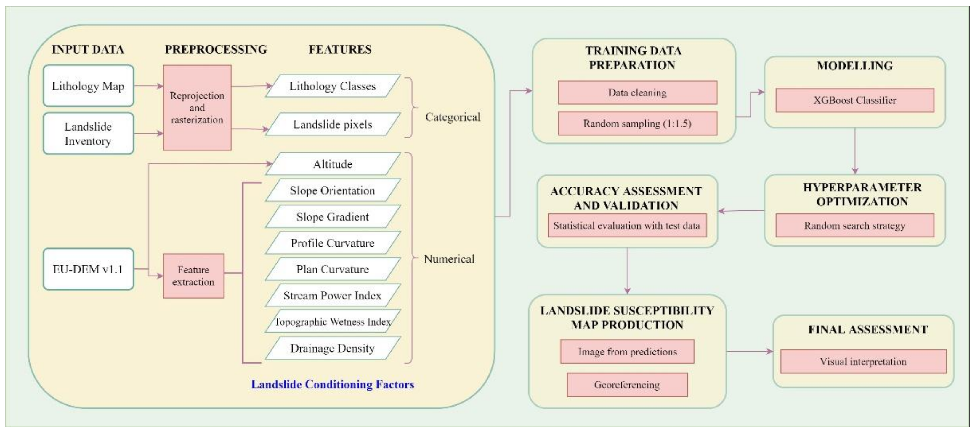
The study area is located in the upper basin of Ataturk Dam and includes Doganyol Town of Malatya, Gerger Town of Adiyaman and Cungus Town of Diyarbakir Province, Turkey. The size of the area is approximately 2718.7 km2. The altitudes range between 525 and 2430 m. Figure 1 shows the location of the study area and the digital elevation model (DEM) cropped from EU-DEM v1.1, which was produced by upgrading EU-DEM v1.0. The EU-DEM v1.1 includes enhancements, which are the correction of geopositioning issues, reducing the artefacts and improving the vertical accuracy of EU-DEM using ice, clouds, and land elevation satellite (ICESat) mission data of National Aeronautics and Space Administration (NASA), U.S.A. as a reference [11]. EU-DEM v1.1 has a nominal resolution of 25 m with vertical accuracy of ±7 m root mean square error (RMSE) [10]. EU-DEM v1.1 was preferred here since it has superior spatial resolution in comparison to the freely available shuttle radar topography mission (SRTM) 30” DEM with 9.7 m RMSE [33]. There exist overall 27 tiles in the EU-DEM v1.1 dataset. Each tile has 25 × 25 m2 cell size and covers 1000 km × 1000 km area defined in the European Terrestrial Reference System 1989—Lambert Azimuthal Equal-Area Europe (ETRS—LAEA) projection with European Petroleum Survey Group (EPSG) Geodetic Parameter Dataset code as 3035. The tile with the ID of E60N20 covers the study area mapped here. This tile was clipped according to the study area extent and employed for further processing. The statistical descriptors of the DEM are provided in Table 1 together with the areal statistics of the landslide inventory, which was obtained from the MTA [5]. The inventory includes 132 landslide polygons in total.
In the southeast of Turkey, between the Mediterranean Sea in the west and the Iran-Iraq border in the east, the geological structure is highly complex due to the closing of two oceanic branches (northern and southern branches of Neo-Tethys) during the Late Cretaceous [34]. As a result of this complexity, they form a nappe-stack, several kilometers-thick, between the Malatya-Keban Metamorphics of the Tauride-Anatolide terrane in the north and the Bitlis-Pütürge Metamorphics of the Arabian Plate in the South [35]. The region is also prone to seismic hazards, which often trigger the landslides [36]. The study area has twenty-seven lithological units in the area as shown in Table 2 and Figure 2. The identifier (ID) numbers shown in Table 2 were assigned to each unit within the study for computational reasons. The frequencies of occurrences in the whole area (Fi) and in the landslide inventory areas (FLi) for each lithological unit are also provided as percentage values in Table 2. Among all lithological units in the study area, only seventeen of them appear in the landslide inventory. The neritic limestone, pelagic limestone, radiolarite, chert and clastics were the most landslide-prone units in the study area. In Figure 3, the numbers of pixels in each lithological unit for the whole area (Figure 3a) and inside the landslide inventory (Figure 3b) are presented. As can be seen in Figure 3 and Table 2, although gneiss, schist type (ID = 11) was the mostly observed lithological unit in the area, neritic limestone type (ID = 5) had the highest amount of landslide pixels followed by the pelagic limestone, clastics, radiolarite, chert, etc. (ID = 12). The metamorphic and magmatic units form the higher altitudes and they were not landslide-prone units.

3.2. Methodology

The overall methodology applied in this study is shown in Figure 4. The workflow consists of data preprocessing for geometric alignment and feature extraction, preparation of the training data for XGBoost algorithm, modeling, hyperparameter optimization, accuracy assessment and validation, LS map production and the final quality assessment via visual interpretation. The methodological details are presented in the following sub-sections.

3.2.1. Data Preprocessing

The main data sources used in this study are the lithology map, the landslide inventory and the DEM. The preprocessing steps can be categorized as: (i) geometric preprocessing and the rasterization of the lithology map; (ii) extraction of topographic derivatives; (iii) preparation of the landslide inventory for the modeling process; (iv) training and test data selection via a random sampling strategy. The lithology map was first transformed into the coordinate reference system of the DEM (ETRS-LAEA with the EPSG code 3035) from the geographical coordinate system WGS84 (EPSG:4326) projection. The vector polygons defining the lithological units were merged to create a single geometry per unit as a preparation step for rasterization. The IDs ranging from one to twenty-seven were used as intensity values in the rasterization process and the rasterized lithology map was produced and stored in the GeoTIFF format. Each pixel in the raster lithology map has a value attribute from one to twenty to represent the lithological units. The coordinate system transformation and the rasterization processes were performed using the open source GDAL/OGR [37] and GeoPandas [38] libraries in the Python3.7 environment.
The topographic derivatives were extracted using the open source SAGA GIS software [39]. The slope orientation, slope gradient, plan and profile curvatures, stream power index (SPI) and the topographic wetness index (TWI) features, which are among the commonly used conditioning factors (e.g., see [15,21,40]) were produced from the DEM. In addition, the drainage density map was produced using the DEM in ArcGIS software from ESRI, Redlands, CA, USA [41]. The SPI was calculated with Equation (1) [42], and shows the erosive power of flowing water [43]. The TWI Equation (2) explains the effect of topography for runoff generation based on the location and the size of source areas [42]. The curvature parameters are the second derivatives of DEMs and define the changes in the first derivatives (i.e., slope gradient and slope aspect) in a certain direction [43].
SPI = A s × tan β
where, As is the catchment area (m2 m−1) and β is the slope gradient (°).
TWI = ln ( A s tan β )
In the third stage regarding the preprocessing of the landslide inventory, five landslides (depicted with the red polygons in Figure 1) were removed from the landslide inventory map for validation purposes. The main idea behind was that the methodology used here classifies landslide and non-landslide samples per pixel and using polygons (or areas) that were not employed for training or testing would allow to analyze the behavior of the classification model better. Thus, only the blue polygons shown in Figure 1 were employed in the training process. The landslide inventory feature used for the model training and testing was the rasterized inventory map, in which each pixel has a value as 0 (non-landslide) or 1 (landslide). The pixels inside the removed landslide polygons have no-data value and thus were not considered in the training step. The rasterization of the landslide inventory map was performed by using the open source GDAL library in Python.
As the last step, for the training and test data selection, index values of the pixels, which were labelled as either landslide or non-landside, were selected and stored separately. The total numbers of landslide and non-landslide pixels were 108,738 and 3,281,991, respectively. A random sampling strategy was applied to non-landslide pixels in order to create a random subset for eliminating the class imbalance problem caused by the small number of landslide pixels. The ratio of landslide/non-landslide pixels was selected as 1:1.5. In the sampling step, the index values of a total of 163,107 non-landslide pixels were selected randomly. The index values of all landslide and the selected non-landslide pixels formed the input training data. Furthermore, all values in this dataset were analyzed and validated for ensuring data quality; 9447 pixels were removed from the training dataset since they fall into the water area. Thus, the final training dataset includes a total of 262,398 observations for each of the nine feature classes.

3.2.2. Modeling with XGBoost and Hyperparameter Optimization

In this study, the XGBoost method [9] was used as the supervised classification model. The method originated from gradient tree boosting algorithm [44,45], which is an effective ML method. It uses regularized boosting technique to reduce the overfitting and thus increase the model accuracy. XGBoost offers scalability for different scenarios, handling of sparse data, availability of comprehensive documentation, low computational resource requirement and high performance (i.e., speed), and the ease of implementation [9]. The method was selected here for being the winner of many data science competitions [9,46]. Further modifications to the method for highly imbalanced datasets also exist (e.g., [47]). It was implemented using the XGBoost Python package [9] in Python 3.7 environment in this study.
XGBoost is an optimized extension of the gradient boosting algorithm. The main idea of a boosting algorithm is combining weak learners outputs sequentially to achieve better performance [48]. XGBoost uses many classification and regression trees (CART) and integrates them using the gradient boosting method. XGBoost has three important aspects, which are regularized objective function for better generalization, gradient tree boosting for additive training, and shrinkage and column subsampling for preventing overfitting [9]. The Equations (3)–(6) summarized from [9] depict the algorithmic process. The XGBoost algorithm aims at minimizing the regularized objective function given in Equation (3).
L ( Φ ) = i l y ^ i , y i + k Ω f k
The first term in Equation (3) is a loss function, which measures the difference between the target y i   and   the   prediction   y ^ i , and the second one is a penalty term as explained in Equation (4) for controlling model complexity to avoid overfitting.
Ω f =   γ T   + 1 2 λ w 2  
where;
  • T: the number of leaves in the tree;
  • w: the score of each leaf;
  • γ , λ   : the regularization degrees.
An iterative approach is applied in the method to minimize the objective function. The objective function to be minimized at step t is given in Equation (5).
L ( t ) = i = 1 n l ( y i , y ^ i ( t 1 ) +   f t ( x i ) ) +   Ω ( f t )  
In order to speed up the optimization process, second order Taylor expansion is applied to the objective. After removing the constant terms, a simplified objective function at step t is given in Equation (6).
L ˜ ( t ) = i = 1 n [ g i f t ( x i ) + 1 2 h i f t 2 x i ] +   Ω f t  
where;
g i = y ^ t 1 l ( y i , y ^ t 1 ) h i = y ^ t 1 2 l ( y i , y ^ t 1 )
In addition to the regularization, shrinkage and feature subsampling are used to prevent overfitting in the XGBoost. There are several algorithms, such as basic exact greedy, approximate, weighted quantile sketch and sparsity-aware split finding, which are available in XGBoost to be used in finding the best split efficiently.
The training dataset prepared in the previous stage was split as training (80%) and testing (20%) sets. The training subset was again divided as training (90%) and validation (10%) sets for the purpose of hyperparameter optimization of the model. The testing dataset (20%) was used for the quality assessment only after the final model was constructed and trained. Although there is no exact criteria or rule of thumb on the ratio selection for the dataset splitting, 70/30 and 80/20 are commonly observed ratios in the literature. The dataset size is an important criterion for this purpose. Since the study dataset was relatively large, the 80/20 approach was followed here and no over- or underfitting was experienced. Due to the large number of hyperparameters to be configured in the XGBoost method, an optimization strategy was needed for improving the performance. Since the random search was found more efficient than the grid based approach [49], it was selected as the hyperparameter optimization method here. First, a parameter space was created; and then the RandomizedSearchCV method implemented in Scikit-learn [50] was utilized to run through the parameter space. Table 3 shows the best parameter values obtained from the hyperparameter optimization process. The SHAP methodology [51,52] was used here to interpret the relationships of the input features with the model predictions.

3.2.3. Accuracy Assessment and Validation

The results of the XGBoost classifier were evaluated using the test dataset. For the assessments, the precision, recall and F1-score were utilized as performance metrics. In addition, receiver operating characteristics (ROC) curve, area under the curve (AUC), confusion matrix and the precision–recall curve were produced for the assessment. Furthermore, a visual inspection by the expert (last author) was carried out in the landslide inventory (the five polygons), which were not used in the modeling. The ROC curve is often used for evaluating classifier’s performance visually [53]. In some situations, such as class imbalance problem, the ROC curve can falsely yield to high performance. The precision-recall curve can give additional information related to the model performance and be a powerful assessment tool when it is evaluated together with the ROC curve [54]. The confusion matrix is a summary of classification performance. Precision, recall, accuracy and F1-score are calculated from the confusion matrix. The AUC is a measure of how well the classifier can distinguish between the classes [53]. The equations used for the calculation of the performance metrics are given in Table 4.

4. Results

4.1. Topographic Derivatives

The descriptive statistics of the topographic derivatives are provided in Table 5. The feature maps together with the respective histograms are provided in Figure 5, Figure 6, Figure 7, Figure 8, Figure 9, Figure 10, Figure 11 and Figure 12. The histograms of the plan curvature (Figure 8) and the SPI (Figure 11) are provided separately for different quantiles of the data in order to increase the readability and interpretability of the information. The statistical and visual analysis are useful to understand the characteristics of the study area, and for assessing the input matrices of the model and the correlations with the output.

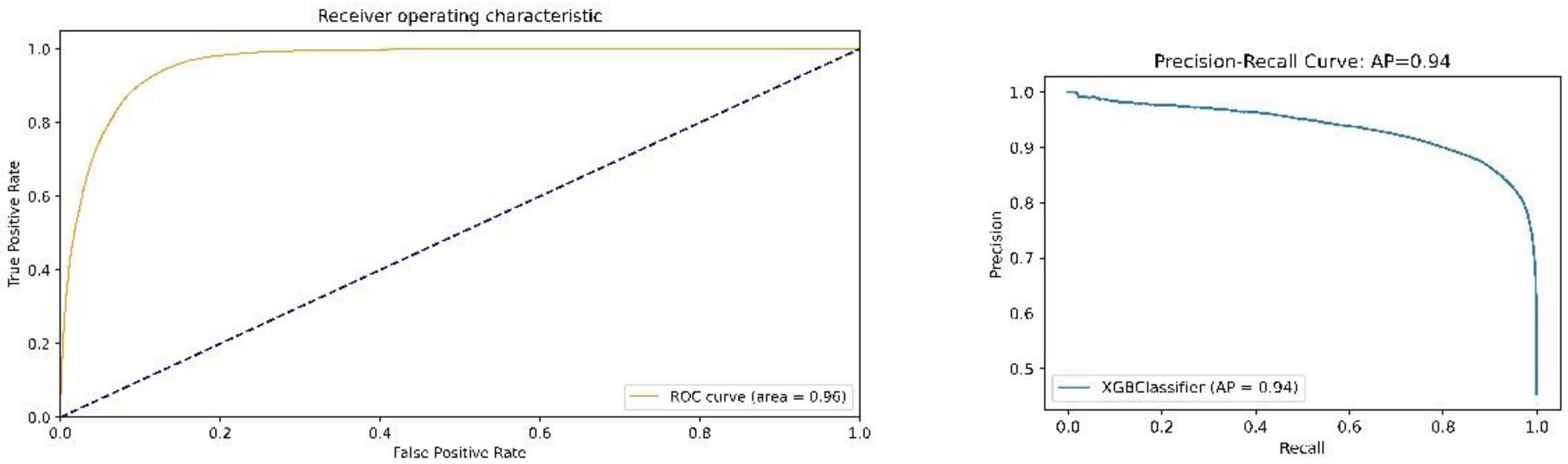
4.2. Prediction Performance Results

The precision, recall and F1-score performance metrics produced by the XGBoost algorithm based on the test dataset are summarized in Table 6. The overall accuracy of the model was 90.18%. As expected, the metrics of the non-landslide class exhibited higher performance. The ROC and the precision–recall curves given in Figure 13 show very high AUC (=0.96) and average precision (AP = 0.94) performances. The normalized confusion matrix presented in Figure 14 show that the false classifications were around 10% for both classes.
Figure 15 shows the SHAP value summary plot, which explains the relationships of the input features with the prediction results. The horizontal axis in the plot shows the magnitude of the effect for each feature given in the vertical axis. The large magnitude values show higher effect. The sign of the value (positive or negative) shows the direction of the correlation. The color codes represent the actual values of the feature as shown in the legend. From Figure 15, it can be interpreted that the lithology and the altitude had larger effects on the prediction results in comparison to the others. The effects of the different lithology types represented by the ID numbers were mixed as can be seen in the graph. The higher altitude values also had influence in the prediction results especially for the higher altitude values. The separation for the higher and lower TWI and the plan curvature values were also obvious as can be seen in the bi-color pattern in the graph. The higher values in TWI and plan curvature were positively correlated with landslide occurrence. Figure 16 shows the feature importance plot. According to the plot, lithology was the most significant among the other features, which means that the lithology feature had high impact on the model predictions, while the profile curvature was being the lowest one.

4.3. LS Map

The final LS map produced in the study is presented in Figure 17. The predicted landslide susceptibility values were classified as very low, low, moderate, high and very high based on the quantile distribution in ArcGIS software from ESRI, Redlands, CA. The black and white polygons plot on the map represent the landslide inventory used for training and final validation, respectively. The results show that even though the landslides used for the final validation only were very large, they can be detected successfully as indicated by the red (very high), orange (high) and yellow (moderate) colors. There were further areas in the upper basin of the dam that were highly susceptible for landsliding and must be monitored carefully.

5. Discussions

When the input features (i.e., the conditioning factors for landslides) in the area were considered, they were sufficient for modeling the susceptibility. The selection of the effective factors are highly dependent on the geoenvironmental settings; here the lithology, altitude and the TWI were determined as the most important ones. Although other conditioning factors can be found in the literature, such as normalized difference vegetation index (NDVI), rainfall, distance to roads, etc.; they were not separable (i.e., differentiating) in the study area and thus were not employed here. On the other hand, even though the topographic derivatives may have multicollinearity, the decision trees and thus XGBoost are known to be immune to this problem [55,56]. Piramithu [56] stated that parameter removal due to multicollinearity problem may yield to lower classification accuracy in decision trees. Additionally, a study by [16] evaluated similar landslide conditioning factors for multicollinearity and showed that the highest correlation value appeared between plan and profile curvatures, which was still below the critical value.
Another important characteristic of the present dataset is the availability of a total of 27 lithological units (Table 2, Figure 3). Among those, ten of them involved no landslide inventory. Considering the potential incompleteness of landslide inventories, which is often the case in the literature, and the lithology being an important feature for susceptibility mapping (see Figure 15 and Figure 16), such areas must be analyzed carefully by experts. Using feature importance metrics in LS studies is recommended for understanding the nature of the problem. In addition, although the land use land cover (LULC) information was not utilized in this study since the region is mostly rural and agricultural with some forest areas; it is recommended to update the LS maps when significant LULC changes occur.
When the overall accuracy values obtained in this study (90.18%) were compared with the results of Pradhan and Kim [28], it was observed the accuracy values here were higher than the XGBoost (76.73%) and the deep neural network accuracy results (83.71%) of the mentioned study. Both the CatBoost (85.03%) and the XGBoost (83.36%) results provided by Sahin [29] are lower than the results obtained here. This situation can be explained by the use of different feature sets (conditioning factors), and the differences in DEM quality and the hyperparameter optimization. It should also be noted that in the present study, the size of the study area (2718.7 km2) was relatively large, which indicates that the results are promising for regional susceptibility assessment studies. On the other hand, when the LS prediction results from recent ML studies carried out in the East and Southeast Anatolia are compared; Karakas et al. [20] obtained AUC values of 0.90 and 0.92 using the RF method in an area of 425 km2 using very high resolution aerial photogrammetric datasets [20]. Sevgen et al. [15] evaluated logistic regression, ANN and RF methods in the close vicinity of a dam reservoir again by using very high resolution aerial photogrammetric datasets; and obtained AUC values of 0.76, 0.84 and 0.95, respectively. Although EU-DEM with lower spatial resolution was used here, the predicted AUC value was 0.96. The high accuracy values can be explained by the prediction power of the XGBoost method and the low noise level in the EU-DEM data.

6. Conclusions and Future Work

In the present study, the XGBoost algorithm was utilized for the LS mapping in the upper basin of Ataturk Dam, a great investment in the Southeast Anatolian part of Turkey. The study area was relatively large (2718.7 km2), which is often a limiting factor in LS mapping. The study area is between the downstream of the Karakaya Dam and the upstream of the Atatürk Dam. In this region, the velocity of the Euphrates River was low and it did not carry too much sediment. However, landslides were likely to contribute to the sediments of the Euphrates River in this section. Therefore, these sediments can cause a decrease in the Atatürk dam reservoir. From this point of view, assessment of the landslide susceptibility of the study area is of particular importance, because there are large landslides in the study area, and it is possible for the displaced and disturbed landslide material to reach the Euphrates River during periods of heavy rainfall. As a result of the study, it was clearly explained that the main factors controlling the landslides in the study area were the lithology, altitude and the TWI. It was clearly demonstrated that using the methodology used here in regional landslide assessment studies produced very useful and promising results.
The performance of the algorithm was high as indicated by various metrics, such as overall accuracy (90.18%), average precision (0.94), F1-score (non-landslide class = 0.92 and landslide class = 0.88) and AUC (0.96). The results show that the XGBoost algorithm and the proposed hyperparameters were successful for the regional LS mapping and can be recommended for future studies. Five landslides, which were not included in the training and modeling stages, could be detected by the proposed algorithm. In addition, the freely available EU-DEM from Copernicus Land Monitoring Service had sufficient quality (i.e., spatial resolution and accuracy) for the purposes of the study.

Author Contributions

Conceptualization and validation, C.G. and S.K.; methodology, S.K., R.C. and C.G.; software, investigation and data curation, R.C.; formal analysis and supervision, S.K.; writing—original draft preparation and visualization, S.K. and R.C.; writing—review and editing, C.G. All authors have read and agreed to the published version of the manuscript.

Funding

This research received no external funding.

Institutional Review Board Statement

Not applicable.

Informed Consent Statement

Not applicable.

Data Availability Statement

Not applicable.

Acknowledgments

The authors sincerely thank Gizem Karakas for her kind support.

Conflicts of Interest

The authors declare no conflict of interest.

References

  1. United Nations Sustainable Development Goals SDG Indicators. E/CN.3/2020/2. Available online: https://unstats.un.org/sdgs/indicators/indicators-list/ (accessed on 4 March 2021).
  2. AFAD. Afet ve Acil Durum Yönetimi Baskanligi Afet Yönetimi Kapsaminda 2019 Yilina Bakis ve Doga Kaynakli Olay Istatistikleri; Technical Report, AFAD, Ankara, Turkey: 7 July 2020. Available online: https://www.afad.gov.tr/kurumlar/afad.gov.tr/e_Kutuphane/Kurumsal-Raporlar/Afet_Istatistikleri_2020_web.pdf (accessed on 4 March 2021).
  3. Cetin, H.; Laman, M.; Ertunc, A. Settlement and slaking problems in the world’s fourth largest rock-fill dam, the Ataturk Dam in Turkey. Eng. Geol. 2000, 56, 225–242. [Google Scholar] [CrossRef]
  4. Akbaş, B.; Akdeniz, N.; Aksay, A.; Altun, İ.; Balcı, V.; Bilginer, E.; Bilgiç, T.; Duru, M.; Ercan, T.; Gedik, İ.; et al. Turkey Geological Map; Mineral Research & Exploration General Directorate: Ankara, Turkey, 2016. [Google Scholar]
  5. MTA Yerbilimleri Harita Goruntuleyici ve Cizim Editorü. Available online: http://yerbilimleri.mta.gov.tr/ (accessed on 4 March 2021).
  6. Yanar, T.; Kocaman, S.; Gokceoglu, C. Use of Mamdani Fuzzy Algorithm for Multi-Hazard Susceptibility Assessment in a Developing Urban Settlement (Mamak, Ankara, Turkey). ISPRS Int. J. Geo-Inf. 2020, 9, 114. [Google Scholar] [CrossRef] [Green Version]
  7. Kocaman, S.; Gokceoglu, C. Possible contributions of citizen science for landslide hazard assessment. Int. Arch. Photogramm. Remote Sens. Spat. Inf. Sci. 2018, 42, 295–300. [Google Scholar] [CrossRef] [Green Version]
  8. Kocaman, S.; Gokceoglu, C. A CitSci app for landslide data collection. Landslides 2019, 16, 611–615. [Google Scholar] [CrossRef]
  9. Chen, T.; Guestrin, C. XG Boost: A scalable tree boosting system. In Proceedings of the 22nd ACM SIGKDD International Conference on Knowledge Discovery and Data Mining-KDD, San Francisco, CA, USA, 13–17 August 2016; ACM Press: New York, NY, USA, 2016; pp. 785–794. [Google Scholar]
  10. European Environment Agency. Copernicus Land Monitoring Service-Reference Data: EU-DEM, Factsheet, May. Available online: https://land.copernicus.eu/user-corner/publications/eu-dem-flyer/at_download/file (accessed on 23 February 2021).
  11. Copernicus Land Monitoring Service. 2021. Available online: https://land.copernicus.eu/ See also: https://land.copernicus.eu/imagery-in-situ/eu-dem/eu-dem-v1.1/view (accessed on 4 March 2021).
  12. Nefeslioglu, H.A.; Gokceoglu, C.; Sonmez, H. An assessment on the use of logistic regression and artificial neural networks with different sampling strategies for the preparation of landslide susceptibility maps. Eng. Geol. 2008, 97, 171–191. [Google Scholar] [CrossRef]
  13. Pourghasemi, H.R.; Pradhan, B.; Gokceoglu, C. Application of fuzzy logic and analytical hierarchy process (AHP) to landslide susceptibility mapping at Haraz watershed, Iran. Nat. Hazards 2012, 63, 965–996. [Google Scholar] [CrossRef]
  14. Regmi, N.R.; Giardino, J.R.; McDonald, E.V.; Vitek, J.D. A comparison of logistic regression-based models of susceptibility to landslides in western Colorado, USA. Landslides 2014, 11, 247–262. [Google Scholar] [CrossRef]
  15. Sevgen, E.; Kocaman, S.; Nefeslioglu, H.A.; Gokceoglu, C. A Novel Performance Assessment Approach Using Photogrammetric Techniques for Landslide Susceptibility Mapping with Logistic Regression, ANN and Random Forest. Sensors 2019, 19, 3940. [Google Scholar] [CrossRef] [Green Version]
  16. Chen, W.; Zhang, S.; Li, R.; Shahabi, H. Performance evaluation of the GIS-based data mining techniques of best-first decision tree, random forest, and naïve Bayes tree for landslide susceptibility modeling. Sci. Total Environ. 2018, 644, 1006–1018. [Google Scholar] [CrossRef]
  17. Mutlu, B.; Nefeslioglu, H.A.; Sezer, E.A.; Akcayol, M.A.; Gokceoglu, C. An experimental research on the use of recurrent neural networks in landslide susceptibility mapping. ISPRS Int. J. Geo-inf. 2019, 8, 578. [Google Scholar] [CrossRef] [Green Version]
  18. Ozer, B.C.; Mutlu, B.; Nefeslioglu, H.A.; Sezer, E.A.; Rouai, M.; Dekayir, A.; Gokceoglu, C. On the use of hierarchical fuzzy inference systems (HFIS) in expert-based landslide susceptibility mapping: The central part of the Rif Mountains (Morocco). Bull. Eng. Geol. Environ. 2020, 79, 551–568. [Google Scholar] [CrossRef]
  19. Karakas, G.; Can, R.; Kocaman, S.; Nefeslioglu, H.A.; Gokceoglu, C. Landslide susceptibility mapping with random forest model for Ordu, Turkey. Int. Arch. Photogramm. Remote Sens. Spat. Inf. Sci. 2020, 43, 1229–1236. [Google Scholar] [CrossRef]
  20. Karakas, G.; Kocaman, S.; Gokceoglu, C. Aerial photogrammetry and machine learning based regional landslide susceptibility assessment for an earthquake prone area in Turkey. Int. Arch. Photogramm. Remote Sens. Spat. Inf. Sci. 2021. accepted. [Google Scholar]
  21. Kocaman, S.; Tavus, B.; Nefeslioglu, H.A.; Karakas, G.; Gokceoglu, C. Evaluation of Floods and Landslides Triggered by a Meteorological Catastrophe (Ordu, Turkey, August 2018) Using Optical and Radar Data. Geofluids 2020, 2020. [Google Scholar] [CrossRef]
  22. Fang, Z.; Wang, Y.; Peng, L.; Hong, H. Integration of convolutional neural network and conventional machine learning classifiers for landslide susceptibility mapping. Comput. Geosci. 2020, 139, 104470. [Google Scholar] [CrossRef]
  23. Achour, Y.; Pourghasemi, H.R. How do machine learning techniques help in increasing accuracy of landslide susceptibility maps? Geosci. Fron. 2020, 11, 871–883. [Google Scholar] [CrossRef]
  24. Chen, W.; Chen, X.; Peng, J.; Panahi, M.; Lee, S. Landslide susceptibility modeling based on ANFIS with teaching-learning-based optimization and Satin bowerbird optimizer. Geosci. Fron. 2021, 12, 93–107. [Google Scholar] [CrossRef]
  25. Chang, S.K.; Lee, D.H.; Wu, J.H.; Juang, C.H. Rainfall-based criteria for assessing slump rate of mountainous highway slopes: A case study of slopes along Highway 18 in Alishan, Taiwan. Eng. Geol. 2011, 118, 63–74. [Google Scholar] [CrossRef]
  26. Lin, H.M.; Chang, S.K.; Wu, J.H.; Juang, C.H. Neural network-based model for assessing failure potential of highway slopes in the Alishan, Taiwan Area: Pre-and post-earthquake investigation. Eng. Geol. 2009, 104, 280–289. [Google Scholar] [CrossRef]
  27. Merghadi, A.; Yunus, A.P.; Dou, J.; Whiteley, J.; ThaiPham, B.; Bui, D.T.; Abderrahmane, B. Machine learning methods for landslide susceptibility studies: A comparative overview of algorithm performance. Earth-Sci. Rev. 2020, 207, 103225. [Google Scholar] [CrossRef]
  28. Pradhan, A.M.S.; Kim, Y.-T. Rainfall-Induced Shallow Landslide Susceptibility Mapping at Two Adjacent Catchments Using Advanced Machine Learning Algorithms. ISPRS Int. J. Geo-Inf. 2020, 9, 569. [Google Scholar] [CrossRef]
  29. Sahin, E.K. Comparative analysis of gradient boosting algorithms for landslide susceptibility mapping. Geocarto Int. 2020, 1–25. [Google Scholar] [CrossRef]
  30. Cao, J.; Zhang, Z.; Du, J.; Zhang, L.; Song, Y.; Sun, G. Multi-geohazards susceptibility mapping based on machine learning—A case study in Jiuzhaigou, China. Nat. Hazards 2020, 102, 851–871. [Google Scholar] [CrossRef]
  31. Arabameri, A.; Chandra Pal, S.; Costache, R.; Saha, A.; Rezaie, F.; Seyed Danesh, A.; Hoang, N.D. Perdition of gully erosion susceptibility mapping using novel ensemble machine learning algorithms. Geomat. Nat. Haz. Risk 2021, 12, 469–498. [Google Scholar] [CrossRef]
  32. Zhang, Y.; Ge, T.; Tian, W.; Liou, Y.A. Debris flow susceptibility mapping using machine-learning techniques in Shigatse area, China. Remote Sens. 2019, 11, 2801. [Google Scholar] [CrossRef] [Green Version]
  33. Mukul, M.; Srivastava, V.; Jade, S.; Mukul, M. Uncertainties in the shuttle radar topography mission (SRTM) Heights: Insights from the indian Himalaya and Peninsula. Sci. Rep. 2017, 7, 1–10. [Google Scholar] [CrossRef] [Green Version]
  34. Sengör, A.M.C.; Yilmaz, Y. Tethyan evolution of Turkey: A plate tectonic approach. Tectonophysics 1981, 75, 181–241. [Google Scholar] [CrossRef]
  35. Ural, M.; Arslan, M.; Göncüoğlu, M.C.; Tekin, U.K.; Kürüm, S. Late Cretaceous arc and back-arc formation within the southern neotethys: Whole-rock, trace element and Sr-Nd-Pb isotopic data from basaltic rocks of the Yüksekova complex (Malatya-Elazığ, SE Turkey). Ofioliti 2015, 40, 57–72. [Google Scholar] [CrossRef]
  36. Karakas, G.; Nefeslioglu, H.A.; Kocaman, S.; Buyukdemircioglu, M.; Yurur, T.; Gokceoglu, C. Derivation of earthquake-induced landslide distribution using aerial photogrammetry: The January 24, 2020, Elazig (Turkey) earthquake. Landslides 2021, 1–17. [Google Scholar] [CrossRef]
  37. GDAL/OGR Contributors. GDAL/OGR Geospatial Data Abstraction Software Library, Open Source Geospatial Foundation. Available online: https://gdal.org (accessed on 3 March 2021).
  38. Jordahl, K.; Van den Bossche, J.; Fleischmann, M.; Wasserman, J.; McBride, J.; Gerard, J.; Tratner, J.; Perry, M.; Badaracco, A.G.; Farmer, C.; et al. Geopandas/Geopandas: V0.8.1 (Version V0.8.1). Zenodo 2020. Available online: http://0-doi-org.brum.beds.ac.uk/10.5281/zenodo.3946761 (accessed on 3 March 2021).
  39. Conrad, O.; Bechtel, B.; Bock, M.; Dietrich, H.; Fischer, E.; Gerlitz, L.; Wehberg, J.; Wichmann, V.; Böhner, J. System for Automated Geoscientific Analyses (SAGA) v. 2.1.4. Geosci. Model. Dev. 2015, 8, 1991–2007. [Google Scholar] [CrossRef] [Green Version]
  40. Gokceoglu, C.; Sonmez, H.; Nefeslioglu, H.A.; Duman, T.Y.; Can, T. The 17 March 2005 Kuzulu landslide (Sivas, Turkey) and landslide-susceptibility map of its near vicinity. Eng. Geol. 2005, 81, 65–83. [Google Scholar] [CrossRef]
  41. ESRI ArcGIS Software. Available online: https://www.esri.com/en-us/arcgis/about-arcgis/overview (accessed on 6 March 2021).
  42. Moore, I.D.; Grayson, R.B.; Ladson, A.R. Digital terrain modeling: A review of hydrological, geomorphological, and biological applications. Hydrol. Process. 1991, 5, 3–30. [Google Scholar] [CrossRef]
  43. Wilson, J.P.; Gallant, J.C. Terrain Analysis Principles and Applications; John Wiley and Sons Inc.: Hoboken, NJ, USA, 2000; ISBN 978-0-471-32188-0. [Google Scholar]
  44. Friedman, J. Greedy function approximation: A gradient boosting machine. Ann. Stat. 2001, 29, 1189–1232. [Google Scholar] [CrossRef]
  45. Friedman, J. Stochastic gradient boosting. Comput. Stat. Data Anal. 2002, 38, 367–378. [Google Scholar] [CrossRef]
  46. Nielsen, D. Tree Boosting with XGBoost-Why Does XGBoost Win “Every” Machine Learning Competition? Master’s Thesis, Department of Mathematical Sciences, Norwegian University of Science and Technology, Trondheim, Norway, 2016. Available online: https://ntnuopen.ntnu.no/ntnu-xmlui/bitstream/handle/11250/2433761/16128_FULLTEXT.pdf (accessed on 3 March 2021).
  47. Wang, C.; Deng, C.; Wang, S. Imbalance-XGBoost: Leveraging weighted and focal losses for binary label-imbalanced classification with XGBoost. Pattern Recogn. Let 2020, 136, 190–197. [Google Scholar] [CrossRef]
  48. Hastie, T.; Tibshirani, R.; Friedman, J.H. 10. Boosting and Additive Trees. In The Elements of Statistical Learning, 2nd ed.; Springer: New York, NY, USA, 2009; pp. 337–384. ISBN 978-0-387-84858-7. [Google Scholar]
  49. Bergstra, J.; Bengio, Y. Random search for hyper-parameter optimization. J. Mach. Learn. Res. 2012, 13, 281–305. [Google Scholar]
  50. Pedregosa, F.; Varoquaux, G.; Gramfort, A.; Michel, V.; Thirion, B.; Grisel, O.; Blondel, M.; Prettenhofer, P.; Weiss, R.; Dubourg, V.; et al. Scikit-learn: Machine learning in Python. J. Mach. Learn. Res. 2011, 12, 2825–2830. [Google Scholar]
  51. Lundberg, S.; Lee, S. A Unified Approach to Interpreting Model Predictions. In NIPS’17: Proceedings of the 31st International Conference on Neural Information Processing Systems; ACM Press: New York, NY, USA, 2017; Volume 1705, pp. 4765–4774. [Google Scholar]
  52. Lundberg, S.M.; Erion, G.; Chen, H.; DeGrave, A.; Prutkin, J.M.; Nair, B.; Katz, R.; Himmelfarb, J.; Bansal, N.; Lee, S.I. From local explanations to global understanding with explainable AI for trees. Nat. Mach. Intell. 2020, 2, 56–67. [Google Scholar] [CrossRef]
  53. Fawcett, T. An Introduction to ROC Analysis. Pattern Recogn. Let. 2006, 27, 861–874. [Google Scholar] [CrossRef]
  54. Davis, J.; Goadrich, M. The Relationship between Precision-Recall and ROC Curves. In Proceedings of the 23rd international conference on Machine learning, Pittsburgh, PA, USA, 25–29 June 2006; pp. 233–240. [Google Scholar]
  55. Kotsiantis, S.B. Decision trees: A recent overview. Artif. Intell. Rev. 2013, 39, 261–283. [Google Scholar] [CrossRef]
  56. Piramuthu, S. Input data for decision trees. Expert Syst. Appl. 2008, 34, 1220–1226. [Google Scholar] [CrossRef]
Figure 1. The location, the digital elevation model (DEM) in hillshade representation and the landslide inventory of the study area.
Applsci 11 04993 g001
Figure 2. Geological map of the study area (reproduced after [4]).
Applsci 11 04993 g002
Figure 3. The pixel counts of lithological units in the (a) study area and (b) landslide inventory area.
Applsci 11 04993 g003
Figure 4. The overall methodological workflow.
Applsci 11 04993 g004
Figure 5. (a) The altitude map (EU-DEM) of the study area and (b) its histogram.
Applsci 11 04993 g005
Figure 6. (a) The slope gradient map of the study area and (b) its histogram.
Applsci 11 04993 g006
Figure 7. (a) The slope orientation (aspect) map of the study area and (b) its histogram. The horizontal axis of the histogram is given in radians.
Applsci 11 04993 g007
Figure 8. (a) The plan curvature map of the study area and (b) its histograms in three quantiles.
Applsci 11 04993 g008
Figure 9. (a) The profile curvature map of the study area and (b) its histogram.
Applsci 11 04993 g009
Figure 10. (a) The TWI map of the study area and (b) its histogram.
Applsci 11 04993 g010
Figure 11. (a) The SPI map of the study area and (b) the histograms of each quantile.
Applsci 11 04993 g011
Figure 12. (a) The drainage density map of the study area and (b) its histogram.
Applsci 11 04993 g012
Figure 13. The ROC curve with AUC = 0.96 (left) and the precision–recall curve with average precision = 0.94 (right).
Applsci 11 04993 g013
Figure 14. Normalized confusion matrix obtained from the study.
Applsci 11 04993 g014
Figure 15. Summary plot of the SHAP values.
Applsci 11 04993 g015
Figure 16. Feature importance plot.
Applsci 11 04993 g016
Figure 17. Landslide susceptibility map produced in the study.
Applsci 11 04993 g017
Table 1. Descriptive statistics of the EU-DEM and the landslide inventory in the study area.
DataMeanStd. DevMin25%50%75%Max
DEM (m)1262.1391.4524.3955.11255.81561.32431.6
Landslide inventory (km2)0.514680.607110.017670.116350.236520.734733.43389
Table 2. Lithological units with the normalized frequency of occurrence.
IDLithological UnitsFi (%)FLi (%)
1Diorite0.2310
2Undifferentiated1.2140
3Non graded terrigenous clastics0.0070
4Sheeted dyke complex1.5200
5Neritic limestone12.54734.146
6Terrigenous clastics1.4039.949
7Volcanites and sedimentary rocks6.8030.237
8Neritic limestone0.8880
9Clastics and carbonates0.4610.510
10Diorite, tonalite, monzonite, gabbro, etc.4.2630.166
11Gneiss, schist32.6992.352
12Pelagic limestone, clastics, radiolarite, chert, etc.5.49123.573
13Basalt, spilite etc.1.5450
14Carbonates and clastics (Upper Cretaceous—Eocene)0.1560.985
15Clastics and carbonates (flysch)1.0750.068
16Clastics and carbonates (Miocene)3.6910.088
17Terrigenous clastics (Miocene)1.7897.197
18Basalt (Upper Miocene)1.6874.321
19Terrigenous clastics (Upper Miocene)0.3280
20Marble3.0080.131
21Undifferentiated basic and ultrabasic rocks6.4851.720
22Terrigenous clastics (Pliocene)2.1600.248
23Non graded terrigenous clastics (Pliocene-Quaternary)1.2940
24Quartzite, quartz schist0.0720
25Carbonates and clastics (Silurian Lower Devonian)0.2960.329
26Pelagic limestone, radiolarite, chert clastics, etc.5.31713.980
27Gabbro3.5710
Table 3. Optimized hyperparameters for the XGBoost method in the study.
HyperparameterDescriptionValue
subsampleSubsample ratio of the observations for each tree0.3
reg_lambdaL2 regularization term3.0
reg_alphaL1 regularization term0.01
n_estimatorsNumber of gradient boosted trees100
min_child_weightMinimum weight to create a new node5
max_depthMaximum depth of a tree10
learning_rateShrinkage factor0.3
gammaRegularization term3
colsample_bytreeSubsample ratio of features for each tree0.5
Table 4. The metrics used for the evaluation of the classification performance. TP: true positive, TN: true negative, FP: false positive and FN: false negative.
Performance MetricEquationEquation Number
Precision TP TP + FP (7)
Recall TP TP + FN (8)
F1-Score 2 Precision Recall Precision   +   Recall (9)
Accuracy TP + TN TP + TN + FP + FN (10)
Table 5. The descriptive statistics of the topographic features in the study area.
FeatureMeanStd.DevMin25%50%75%Max
Slope Orientation (radian)3.2921.7910.0001.8983.1564.9516.283
Drainage Density5.0866.7260.0000.0002.5967.69476.997
Plan Curvature0.00010.0440−29.6834−0.00360.00010.004224.9625
Profile Curvature−0.00010.0023−0.1168−0.00090.00000.00090.0399
Slope Gradient0.2840.1640.0000.1610.2700.3901.252
SPI6593.045,812.10394.61164.22894.05,984,523.5
TWI7.1662.5832.4455.6706.4667.70726.575
Table 6. Performance metrics of the model.
ClassPrecisionRecallF1-ScoreSupport
Non-Landslide0.930.900.9231,070
Landslide0.860.910.8821,410
Publisher’s Note: MDPI stays neutral with regard to jurisdictional claims in published maps and institutional affiliations.

