1. Introduction
Constant demand exists for permanent accuracy improvement in machine tool manufacturing technology, aiming to eliminate errors caused by different deformations. There are two approaches to solving this problem. First, all sources of erroneous movements can be considered to produce perfect equipment with a reasonable assignment of stiffness, and optimal addition of damping, material selection, and symmetrical structure design [
1,
2]. In this case, regardless of how well a machine may be designed, the accuracy is limited because of thermal or other deformations that are not accounted for [
3]. Alternatively, it is possible to analyze erroneous movements and eliminate them with compensation [
4]. This technique allows the accuracy to be increased even for a moderately accurate machine tool.
The causes of errors were analyzed and classified in [
5]. The authors distinguished three sources of errors: geometric and kinematic errors, thermal errors, and cutting force errors. The most significant factor is the thermal error, which causes 40–70% of machine tool errors [
6]. It is known that up to 75% of overall geometrical errors can be induced by thermal effects [
7]. The sources of thermal influence are listed in [
6]: heat caused by the cutting process; heat generated in the machine system due to friction, engines, etc.; heating or cooling provided by the cooling system; and thermal memory from the previous state. The machine’s moving parts generate heat, which results in an inaccurate position of the cutting tool end in the thermoplastic machine system. These erroneous movements are unavoidable and significantly affect the accuracy [
5].
Error compensation consists of choosing a model, determining the optimal position of the sensors, measuring each of the error components, determining the current position of the instrument and temperature, calculating corrective actions, and reducing the deviation. The first step in this list is choosing a thermal model and quantitatively estimating the machine part’s thermal characteristics. Ref. [
8] reviews the actual methods of machine tool modeling: linear polynomial models, neural network models, approaches based on linear regression analysis, probabilistic methods, frequency domain analysis, and others. The authors propose the linear state-space representation of the lumped mathematical model.
A promising approach to predicting temperature distribution and estimating thermal errors is to use models of systems with distributed parameters. Distributed parameter thermal models have been found to predict temperature distribution and estimate thermal errors with high accuracy. The heating and cooling devices also may be arranged for temperature stabilization. The calculation of the temperature error can also be performed based on measurements and a dynamic model, and used to calculate corrective movements by applying the actuators.
In most cases, we are interested in improving the main assemblies, for example, spindle or feed, so we can use the models of these assemblies, which is much less time consuming [
7]. The models of assemblies in PDE form consider their distributed nature and allow them to be described with higher accuracy.
Heat transfer coefficients may vary with time, and their variations can be random or periodic [
9]. The factors that influence the heat transfer coefficient are the temperature distribution of the structure, ambient effects, and temperature-dependent material properties [
10]. In the case of preliminary assessment of system behavior based on analytical solutions, time-varying parameters make the PDE nonstationary and difficult for analytical analysis. In [
11], the influence of the transfer coefficient values on the machine tool thermal behavior is investigated, and the changing convection regime is observed using finite element method simulation. It is shown that the machine error depends on the transfer coefficient.
Different methods of distributed systems analysis exist. For example, in [
12,
13,
14] heat transfer process analysis using the finite difference method is considered. In [
15,
16,
17] the problem of heat conduction is solved using polynomial approximation. The authors show that their solution is more accurate than the solution obtained by the finite difference method. Refs. [
18,
19,
20] considers the solution of the heat conduction problem by the perturbation method. The disadvantages of these methods are a very rapid increase in computational complexity with a rise in the problem dimension and the limited application area. According to [
8], the use of the finite element method is limited for a number of reasons, including environmental factors such as variable room temperature conditions or convection coefficients.
The study of methods for analyzing temperature fields based on models in PDE form allows us to draw the following conclusion: although it is preferable to use a model that is not overly complicated, this model should consider most of the possible effects. A similar deduction is beautifully illustrated in [
21]. The standard complexes based on the finite element method facilitate simulation of the spindle geometry, but they are computationally expensive. It is preferable to have an effective thermal model for analyzing the system behavior at an early stage of development.
This paper describes an approach for the analysis of a distributed system. It is proposed to pass from a PDE to an indefinite system of linear algebraic equations for the coefficients of the Fourier series for the temperature function, using the spectral method [
22], and, in some cases, reduce the number of computational operations. This method allows investigating the models with the coefficients dependent on time. The proposed method has the advantage of analytical solution methods because it provides information about the model’s temperature at any point. In contrast, numerical methods make it possible to calculate the temperature only at preselected points.
2. Mathematical Model of the System
The mathematical model of transient heat transfer is based on a boundary value problem with some restrictions:
The spindle bearings are the source of the most active heat generation and heat supply to the spindle. They are considered in the model as boundary conditions of the second kind.
Heat radiation to the surrounding is ignored.
The temperature depends only on the axial spatial variable. It is possible to expand the model and take into account the dependence of temperature on the radial coordinate [
22]. In this case, the mathematical description of the complex shape is represented as the system of PDEs with the corresponding boundary conditions. This restriction does not limit the proposed analysis method but greatly simplifies calculations and allows a graphic result to be obtained.
To ensure the similarity of thermal processes and the model under the third assumption, the dimension parameters of the model should be chosen such that the Biot and Fourier coefficients are the same for the model and the structure [
23].
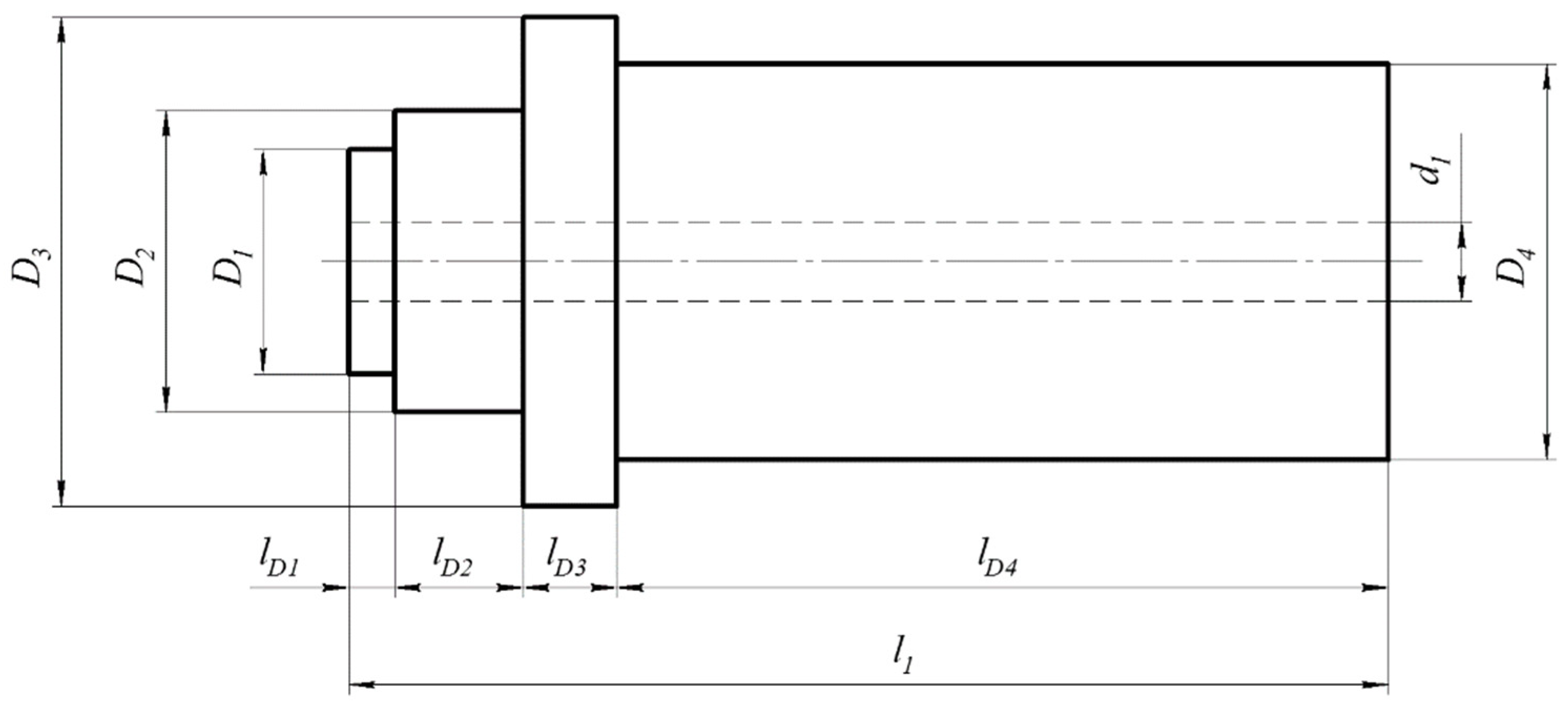
Thermal model length and spindle length are equal. The following expression allows calculation of the diameter of the equivalent cylinder used in the model [
23]:
where
k is the number of spindle sections of the same outer diameter,
m is the number of spindle sections of the same inner diameter,
Di is the outer diameter of the
i-th section,
dj is the inner diameter of the
j-th section,
is the section length with the same inner or outer diameter.
One of the possible spindle configurations is shown in
Figure 1. In the case of
,
,
,
,
,
,
,
,
,
, the calculations by Expression (1) give
.
Under the mentioned restrictions, the mathematical model of heat distribution is a heat-conduction equation [
23]:
with boundary conditions of the second kind:
and the initial condition:
where
T is the temperature,
t is the time,
x is the spatial variable,
L is the length of the model,
a is the thermal diffusivity,
α(
t) is the time-dependent heat-transfer coefficient,
λ is the thermal conductivity,
are heat flux in the rear and front supports,
F is the cross-sectional area of a cylinder,
d is the diameter of the model.
The representation of the Equations (2)–(4) in the dimensionless form:
where
,
,
are the dimensionless variables
are the time and temperature scaling factors,
.
Boundary conditions:
where
,
are the relative heat fluxes,
Q is the scaling factor.
In [
23], the solution of Equation (5) with boundary conditions of Equation (6) and
is obtained by the operational calculus in the form of a series for the case when
are constants or change exponentially over time. The choice of the exponential functions is explained by the changing in the value of the clearance (interference). As a result, the amount of generated heat also changes over time, close to an exponential law.
Consider the case when the heat fluxes at the boundaries change exponentially:
that is:
Note that, in solving the problem by the spectral method, the boundary condition functions do not necessarily have to change exponentially.
3. The Spectral Form of the Mathematical Model
We obtain the spectral form representation of the system (5)–(7). Representing the function
in the form of a Fourier series in the system of orthonormal differential functions
:
Representing the function
with zero initial conditions (Equation (7)) in the form:
where the function
θ0(
ξ,
τ) coincides with the function
θ(
ξ,
τ) in the domain
;
are amplitudes of step functions, operating on the boundaries
and
, respectively.
The first-time derivative of Function (11) is determined by the expression [
24]:
where
.
To provide the correct expression for the second spatial derivative, the first spatial derivative is represented in the form:
where
coincides with the function
in the domain
. Thus, the second spatial derivative has the form:
where
are the amplitudes of the jumps of the first derivative of the functions operating on the boundaries
and
, respectively.
When we have the boundary conditions of the second kind, Expression (14) is transformed as:
For each of the components of Equation (5), the spectral form is obtained considering Expressions (12) and (15).
According to [
22], the spectral characteristic of the derivative
in the case of the boundary conditions of the second kind has the form:
where
is the vector of the spectral characteristic with respect to the spatial and temporal variables, the index
i of this vector is calculated as
;
is the operating differentiation matrix of second-order for the variable
ξ, defined as the tensor product:
where
is the operating differentiation
matrix of second-order
, with the elements calculated by the expression:
is the identity
matrix
;
are vectors of boundary conditions of the second kind, determined by the expressions:
is the vector composed of functions of the System (9); are vectors of spectral characteristics of the functions .
The spectral characteristic of the derivative
with zero initial conditions has the form [
22]:
where:
is the operating differentiation
matrix of the first-order
, with the elements calculated by the expression:
Let us note that we have only one term in Expression (20) of the time derivative’s spectral characteristic which corresponds to the spectral characteristic of . The spectral characteristics of the terms are equal to zero.
The spectral characteristic of the term
has the form [
22]:
where
is the operating matrix of the factor
, defined as the tensor product:
is the
-matrix
, with the elements calculated by the expression:
Thus, we have an infinite system of algebraic equations written for the vector of the space-time spectral characteristic
:
System (26) can be represented as:
The solution of this system is determined by the expression:
The reverse transition to the function θ(ξ,τ) is carried out using the Fourier series by Expression (10).
4. Example
Let us calculate matrices of the spectral representation in Equation (27) for the System (2)–(4) with parameters
,
,
,
,
,
,
,
[
23]. As scaling factors, we choose
,
. Then
.
Equation (5) of the system in dimensionless form is:
The boundary conditions (Equation (6)) are in the form:
As a decomposition system in the variable
ξ, we use the system of functions:
orthonormal on the interval
. As a decomposition system in the variable
τ, we use the system of functions:
orthonormal on the interval
. The choice of expansion functions is determined by the intended form of decision and by the fact that vectors of boundary conditions of the second kind (Equation (19)) should be non-zero.
The operating differentiation matrices
computed by the Expressions (17) and (21), respectively, for the selected decomposition Systems (32), (33), are:
In the case of constant heat transfer coefficient, the operating matrix
is defined as
. We obtain vectors
by Expression (19). The matrices of the composed System (27) are determined by the calculated matrices
and are not shown due to their high dimension. After computing the spectral characteristic vector
, according to Equation (28) it is possible to construct a function
θ(
ξ,
τ) by the expression:
The number of terms in Equation (36) should provide the required accuracy estimated by the expression:
where
is the exact solution,
is the solution in the form of Equation (36).
In general, the exact solution is unknown but we can use the analytical solution defined for some special cases. For example, in the case of a constant heat transfer coefficient, we can use the expression for the analytical solution
defined via Green’s function [
25]:
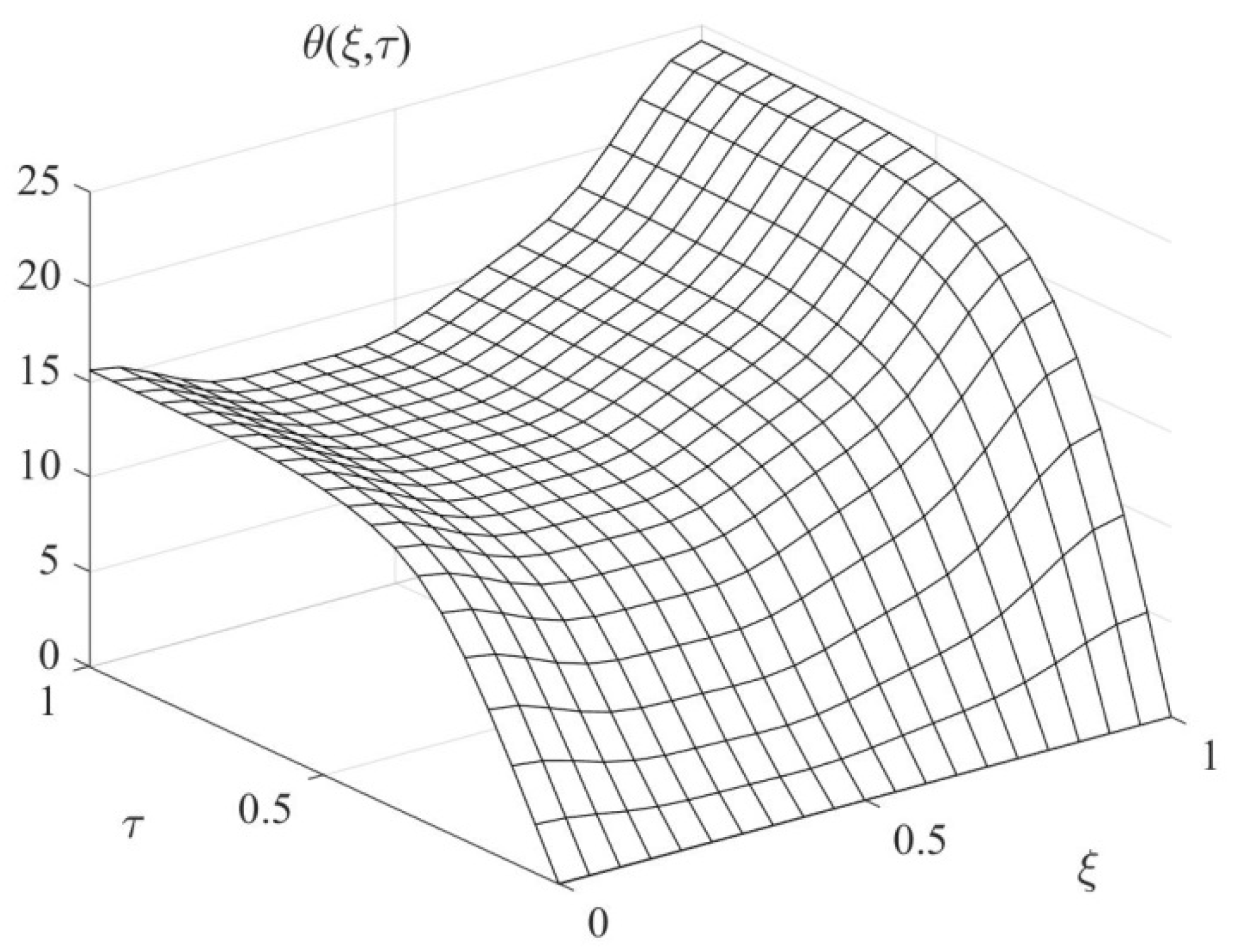
The accuracy of the solution of Equation (36) with
and 9 terms of Equation (38) taken into account:
. The simulation results in MATLAB for
and constant heat transfer coefficient are shown in
Figure 2.
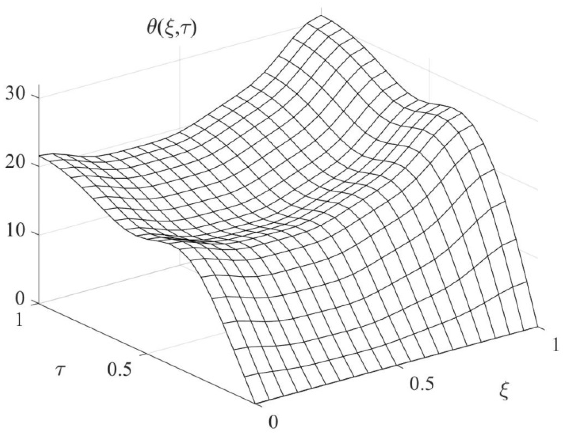
Let us consider the case when
is time variable:
In this case the operating matrix
is defined as:
The simulation results for
and variable heat transfer coefficient are shown in
Figure 3.
This method is applicable for the heat conduction in case of two or three spatial variables, with mixed type boundary conditions and a time-dependent heat transfer coefficient.
5. Conclusions
For preliminary analysis of a temperature field in a machine assembly, taking into account the environmental thermal fluctuations surrounding a machine tool, the thermal model in the PDE form was used. This model describes the heat transfer in the spindle by the PDE, where the temperature depends only on the axial spatial variable. The similarity of the process and the model is achieved by choosing the generalized diameter, such that the Biot and Fourier coefficients would be the same for the model and the structure. The spindle bearings are considered in the model as boundary conditions of the second kind. The environmental thermal fluctuations are described by the time-dependent heat transfer coefficient in the PDE.
Based on the spectral method, the decomposition of the temperature function in a Fourier series for the axial coordinate and time allows representing the PDE as an infinite system of linear algebraic equations. The set of variables of this system represents the amplitudes of spatial modes. This solution has the following advantages: the temperature can be calculated at any point, as in analytical results; and it is possible to evaluate the influence of the environment by adding time dependency of the heat transfer coefficient. The accuracy of the obtained solution is investigated in the case of the constant heat transfer coefficient.
In the case of the modeling of spindle temperature, it is essential to first check the maximum spindle temperature, which characterizes the operation of the spindle bearings. The method is applicable for preliminary analysis of the thermal characteristics for other basic machine parts. The proposed method can be used for temperature field analysis in 2D and 3D constructions. An example of solving analysis and synthesis problems for a 2D distributed object is represented in [
22].


