ALPINE: Active Link Prediction Using Network Embedding

Abstract

Many real-world problems can be formalized as predicting links in a partially observed network. Examples include Facebook friendship suggestions, the prediction of protein–protein interactions, and the identification of hidden relationships in a crime network. Several link prediction algorithms, notably those recently introduced using network embedding, are capable of doing this by just relying on the observed part of the network. Often, whether two nodes are linked can be queried, albeit at a substantial cost (e.g., by questionnaires, wet lab experiments, or undercover work). Such additional information can improve the link prediction accuracy, but owing to the cost, the queries must be made with due consideration. Thus, we argue that an active learning approach is of great potential interest and developed ALPINE (Active Link Prediction usIng Network Embedding), a framework that identifies the most useful link status by estimating the improvement in link prediction accuracy to be gained by querying it. We proposed several query strategies for use in combination with ALPINE, inspired by the optimal experimental design and active learning literature. Experimental results on real data not only showed that ALPINE was scalable and boosted link prediction accuracy with far fewer queries, but also shed light on the relative merits of the strategies, providing actionable guidance for practitioners.

1. Introduction

Network embedding and link prediction: Network embedding methods [1], also known as graph representation learning methods, map nodes in a graph onto low-dimensional real vectors, which can then be used for downstream tasks such as graph visualization, link prediction, node classification, and more. Our focus in this paper was on the important downstream task of link prediction.

The purpose of link prediction in networks is to predict future interactions in a temporal network (e.g., social links among members in a social network) or to infer missing links in static networks [2]. Applications of link prediction in networks range from predicting social network friendships, consumer-product recommendations, citations in citation networks, to protein–protein interactions. While classical approaches for link prediction [3] remain competitive for now, link prediction methods based on the state-of-the-art network embedding methods already match and regularly exceed them in performance [4].

Active learning for link prediction: An often-ignored problem affecting all methods for link prediction, and those based on network embedding in particular, is the fact that obtaining information on the connectivity of a network can be challenging, slow, or expensive. As a result, in practice, networks are often only partially observed [5], while for many node pairs, the link status remains unknown. For example, an online consumer-product network is far from complete as the consumption offline or on other websites is hard to track; some crucial relationships in crime networks can be hidden intentionally; in biological networks (e.g., protein interaction networks), wet lab experiments may have established or ruled out the existence of links between certain pairs of biological entities (e.g., interactions between proteins), while due to limited resources, for most pairs of entities, the link status remains unknown. Moreover, in many real-world networks, new nodes continuously stream in with very limited information on their connectivity to the rest of the network.

In many of these cases, a budget is available to query an “oracle” (e.g., human or expert system) for a limited number of as-yet unobserved link statuses. For instance, wet lab experiments can reveal missing protein–protein interactions, and questionnaires can ask consumers to indicate whether they have seen particular movies before or have a friendship relation with a particular person. Of course, the link statuses of some node pairs are more informative than those of the others. Given the typically high cost of such queries, it is thus of interest to identify those node pairs for which the link status is unobserved, but for which knowing it would add the most value. Obviously, this must be performed before the query is made and thus before the link status is known.

This kind of machine learning setting, where the algorithm can decide for which data points (here: node pairs) it wishes to obtain a training label (here: link status), is known as active learning. While active learning for the particular problem of link prediction is not new [6,7,8,9], it has received far less attention than active learning for standard classification or regression problems, and the use of active learning for link prediction based on network embedding methods has to the best of our knowledge remained entirely unexplored. Studying this is the main aim of this paper: Can we design active learning strategies that identify the node pairs with unobserved link status, of which knowing the link status would be maximally informative for the network embedding-based link prediction? To determine the utility of a candidate node pair, we focused on the link prediction task: querying a node pair’s link status is deemed more useful if the embedding found with this newly obtained link status information is better for the important purpose of link prediction.

Partially observed networks: To solve this problem, a distinction should be made between node pairs that are known to be unlinked and node pairs for which the link status is not known. In other words, the network should be represented as a partially observed network, with three node pair statuses: linked, unlinked, and unknown. The node pairs with unknown status are then the candidates for querying, and if the result of a query indicates that they are not linked, actual information is added. This contrasts with much of the state-of-the-art in network embedding research, where unlinked and unknown statuses are not distinguished.

Thus, the active learning strategies proposed will need to build on a network embedding method that naturally handles partially observed networks. Given such a method, we then need an active learning query strategy for identifying the unknown candidate link statuses with the highest utility. After querying the oracle for the label of the selected link status, we can use it as additional information to retrain the network embedding model. In this way, more and more informative links and non-links become available for training the model, maximally improving the model’s link prediction ability with a limited number of queries.

The ALPINE framework: We proposed the ALPINE (Active Link Prediction usIng Network Embedding) framework, the first method using active learning for link prediction based on network embedding, and developed different query strategies for ALPINE to quantify the utilities of the candidates. Our proposed query strategies included simple heuristics, as well as principled approaches inspired by the active learning and experimental design literature. ALPINE was based on a network embedding model called Conditional Network Embedding (CNE) [10], whose objective function is expressed analytically. There are two reasons why we chose to build our work on CNE. The first is that, as we will show, CNE can be easily adapted to work for partially observed networks, as opposed to other popular network embedding methods (including those based on random walks). The second reason is that CNE is an analytical approach (not relying on random walks or sampling strategies), and thus allowed us to derive mathematically principled active learning query strategies. Yet, we note that ALPINE can be applied also to other existing or future network embedding methods with these properties.

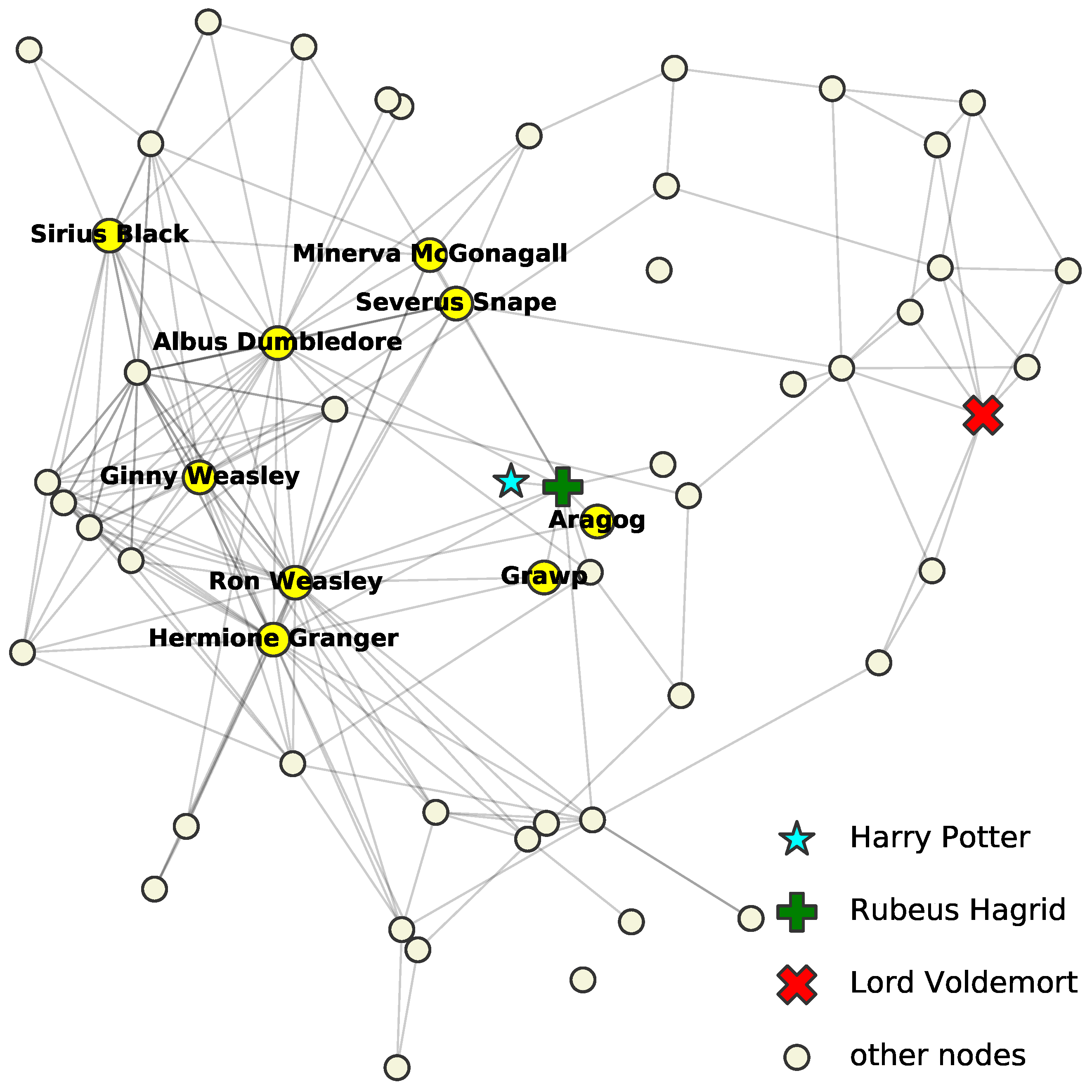
Illustrative example: To illustrate the idea of ALPINE, we give an example on the Harry Potter network [11]. The network originally had 65 nodes and 223 ally links, but we only took its largest connected component of 59 characters and 218 connections. Note that enemy relation was not considered. We assumed that the network was partially observed: the links and non-links for all characters except “Harry Potter” (the cyan star) were assumed to be fully known, and for Harry Potter, only his relationship with “Rubeus Hagrid” (the green plus) was observed as linked and with “Lord Voldemort” (the red x) as unlinked. The goal was to predict the status of the unobserved node pairs, i.e., whether the other nodes (the circles) were allies of “Harry Potter”. Suppose we have a budget to query five unobserved relationships. We thus want to select the five most informative ones.

ALPINE can quantify the informativeness of the unknown link statuses, using different query strategies. Shown in

Table 1. Top 5 query selections for the three strategies of ALPINE.

Strategy	Max-Deg.	Max-Prob.	Max-Ent.
1	Ron Weasley	Ron Weasley	Albus Dumbledore
2	Albus Dumbledore	Hermione Granger	Grawp
3	Hermione Granger	Albus Dumbledore	Minerva McGonagall
4	Ginny Weasley	Grawp	Severus Snape
5	Sirius Black	Minerva McGonagall	Aragog

are the top five queries selected by strategies max-deg., max-prob., and max-ent., which are defined in Section 4. Nodes mentioned in the table are highlighted with character names in Figure 1. Strategy max-deg. suggests to query the relationships among Harry and the high-degree nodes—those who are known to have many allies. Strategy max-prob. selects nodes that are highly likely to be Harry’s friends based on the observed part of the network. Finally, max-ent. proposes to query the most uncertain relationships. A more detailed discussion of these results and a thorough formal evaluation of ALPINE are left for Section 5, but the reader may agree that the proposed queries are indeed intuitively informative for understanding Harry’s social connections.

Contributions. The main contributions of this paper are:

• We proposed the ALPINE framework for actively learning to embed partially observed networks by identifying the node pairs with an as-yet unobserved link status of which the link status is estimated to be maximally informative for the embedding algorithm (Section 3).
• To identify the most informative candidate link statuses, we developed several active learning query strategies for ALPINE, including simple heuristics, uncertainty sampling, and principled variance reduction methods based on D-optimality and V-optimality from experimental design (Section 4).
• Through extensive experiments (the source code of this work is available at https://github.com/aida-ugent/alpine_public, accessed on 17 October 2020), (1) we showed that CNE adapted for partially observed networks was more accurate for link prediction and more time efficient than when considering unobserved link statuses as unlinked (as most state-of-the-art embedding methods do), and (2) we studied the behaviors of different query strategies under the ALPINE framework both qualitatively and quantitatively (Section 5).

2. Background

Before introducing the problem we studied and the framework we proposed, in this section, we first survey the relevant background and related work on active learning and network embedding.

2.1. Active Learning and Experimental Design

Active learning is a subfield of machine learning, which aims to exploit the situation where learning algorithms are allowed to actively choose (part of) the training data from which they learn, in order to perform better. It is particularly valuable in domains where training labels are scarce and expensive to acquire [12,13,14], and thus where a careful selection of the data points for which a label should be acquired is important. The success of an active learning approach depends on how much more effective its choice of training data is, when compared to random acquisition, also known as passive learning. Mapped onto the context of our work, the unlabeled “data points” are node pairs with an unknown link status, and an active learning strategy would aim to query the link statuses of those that are most informative for the task performed by the network embedding model. Of particular interest to the current paper is pool-based active learning, where a pool of unlabeled data points is provided, and a subset from this pool may be selected by the active learning algorithm for labeling by a so-called oracle (this could be, e.g., a human expert or a biological experiment). In the present context, this would mean that the link status of only some of the node pairs can be queried.

Active learning is closely related to optimal experimental design in statistics [15], which aims to design optimal “experiments” (i.e., the acquisition of training labels) with respect to a statistical criterion and within a certain cost budget. The objective of experimental design is usually to minimize a quantity related to the (co)variance matrix of the estimated model parameters or of the predictions this model makes on the test data points. In models estimated by the maximum likelihood principle, a crucial quantity in experimental design is the Fisher information: it is the reciprocal of the estimator variance, thus allowing one to quantify the amount of information a data point carries about the parameters to be estimated.

While studied for a long time in statistics, the idea of estimator variance minimization first showed up in the machine learning literature for regression [16], and later, the Fisher information was used to judge the asymptotic values of the unlabeled data for classification [17]. Yet, despite this related work in active learning and the rich and mature statistical literature on experimental design for classification and regression problems, to the best of our knowledge, the concept of variance reduction has not yet been studied for link prediction in networks or network embedding.

2.2. Network Embedding and Link Prediction

The confluence of neural network research and network data science has led to numerous network embedding methods being proposed in the past few years. Given a (undirected) network $\mathcal{G}=(V,E)$ with nodes V and edges $E\subseteq \left(\genfrac{}{}{0pt}{}{V}{2}\right)$, the goal of a network embedding model is to find a mapping $f:V\to {\mathbb{R}}^d$ from nodes to d-dimensional real vectors. The embedding of a network is denoted as $\mathit{X}={\left[{\mathit{x}}_1,{\mathit{x}}_2,\dots ,{\mathit{x}}_n\right]}^T\in {\mathbb{R}}^{n\times d}$. In short, network embedding methods aim to find embeddings such that first-order [10] or sometimes higher order [18,19] proximity information between nodes is well approximated by some distance measure between the embeddings of the nodes. In this way, they aim to facilitate a variety of downstream network tasks, including graph visualization, node classification, and link prediction.

For the link prediction task, a network embedding model uses a function $g:{\mathbb{R}}^d\times {\mathbb{R}}^d\to \mathbb{R}$ evaluated on ${\mathit{x}}_i$ and ${\mathit{x}}_j$ to compute the probability of nodes i and j being linked. In practice, g can be found by training a classifier (e.g., logistic regression) on a set of linked and unlinked node pairs, while it can also follow directly from the network embedding model. The method CNE, on which most of the contributions in the present paper were based, belongs to the latter type. With $\mathbf{A}\in {\{0,1\}}^{n\times n}$ the adjacency matrix of a network $\mathcal{G}=(V,E)$ (i.e., $a_{ij}=1$ if $\{i,j\}\in E$ and zero otherwise), the goal of CNE is to find an embedding, denoted as ${\mathit{X}}^{*}$, that maximizes the probability of the network given that embedding [10]:

$$\begin{array}{c}\hfill P\left(\mathcal{G}\right|\mathit{X})=\prod _{\{i,j\}\in E}P(a_{ij}=1|\mathit{X})·\prod _{\{k,l\}\notin E}P(a_{kl}=0|\mathit{X}),\end{array}$$

(1)

where $P(a_{ij}=1|\mathit{X})=g({\mathit{x}}_i,{\mathit{x}}_j)$ for a suitably defined g (see [10] for details).

A problem with all existing network embedding methods we are aware of is that they treat unobserved link statuses in the same way they treat unlinked statuses. For example, in methods based on a skip gram with negative sampling, such as DeepWalk [18] and node2vec [19], the random walks for determining node similarities traverse via known links, avoiding the unobserved node pairs and thus treating them in the same way as the unlinked ones. Similarly, the more recently introduced Graph Convolutional Networks (GCNs) [20] allow nodes to recursively aggregate information from their neighbors, again without distinguishing unobserved from unlinked node pair statuses. We argue that this makes existing methods suboptimal for link prediction in the practically common situation when networks are only partially observed. This has gone largely unnoticed in the literature, probably because partially observed networks do not tend to be used in the empirical evaluation setups in the papers where these methods were introduced.

The failure to recognize the crucial distinction between unobserved and unlinked node pair statuses has also precluded research on active learning in this context. Indeed, the pool will be a subset of the set of unobserved node pairs, and an unlinked result of a query will add value to the embedding algorithm only if the unobserved status was not already treated as unlinked. Thus, in order to do active network embedding for link prediction, it is essential to distinguish the two links’ status.

While CNE was not originally introduced for embedding partially observed networks, it is easily adapted for this purpose (this is not the case, e.g., for skip gram-based methods based on random walks). We will show how this is performed in Section 3.1. This is an important factor contributing to our choice for using this model in this paper.

2.3. Related Work

Our work sits at the intersection of three topics: active learning, network embedding, and link prediction. There exists work on the combinations of any two, but not all three of them. Most prominently, link prediction is a commonly considered downstream task of network embedding [1], but active learning has not been studied in this context. Research on active network embedding has focused on node classification [13,21,22], but link prediction was not considered as a downstream task in this literature. Finally, active learning for link prediction is not new either [6,7,9], but so far, it has been studied in combination with more classical techniques than network embedding. Thus, to the best of our knowledge, the present paper is the first one studying the use of active learning for network embedding with link prediction as a downstream task. Given the promise network embedding methods have shown for link prediction, we believe this is an important gap to be filled.

Work on active learning for graph-based problems has focused on node and graph classification, as well as on various tasks at the link level [14,23]. The graph classification task considers data samples as graph objects, useful, e.g., for drug discovery and subgraph mining [24], while the node classification aims to label nodes in graphs [25,26,27,28]. Active learning has also been used for predicting the sign (positive or negative) of edges in signed networks, where some of the edge labels are queried [6]. Similarly, given a graph, Jia et al. [8] studied how edge flows can be predicted by actively querying a subset of the edge flow information, to help with sensor placement in water supply networks. All these methods are only laterally relevant to the present paper, in that their focus is not on link prediction.

The methods most strongly related to our work are ActiveLink [7] and HALLP [9].

ActiveLink is designed for link prediction in knowledge graphs and has as its aim to speed up the training of the deep neural link predictors by actively selecting the training data [7]. More specifically, the method selects samples from the multitriples constructed according to the training triples. As link prediction in a knowledge graph with only one relation (one predicate) is equivalent with link prediction in a standard graph as considered in this paper, ActiveLink appears to be a meaningful baseline for our paper. However, when applied to a standard graph in this way, ActiveLink would work by querying all node pairs involving a set of selected nodes (or, in terms of the adjacency matrix, it would query entire rows or columns). Thus, this strategy would learn the entire neighborhood of the selected nodes, but very little about the rest of the network. While this strategy may be sensible in the case of a knowledge graph where information about one relation may also be informative about other relations, it is clearly not useful for standard graphs. This excludes ActiveLink as a reasonable baseline.

HALLP, on the other hand, proposes an active learning method for link prediction in standard networks [9], demonstrating a benefit over passive learning. However, both HALLP’s link prediction method (based on a support vector machine [29]) and its active learning query strategy utilize a pre-determined set of features rather than a learned model such as a network embedding. The query strategy attempts to select node pairs for which the link prediction is most uncertain. Specifically, HALLP considers two link prediction models for calculating these uncertainties for the candidate node pairs, defining the utility of a candidate node pair as follows:

$$\begin{array}{c}\hfill u_{\mathit{A}}(i,j)=c_1{u}_{local}(i,j)+c_2{u}_{global}(i,j).\end{array}$$

(2)

Here, $u_{local}(i,j)$ is the so-called local utility that measures the uncertainty of a linear SVM link prediction model, $u_{global}(i,j)$ is the so-called global utility based on the hierarchical random graph link predictor [30], and $c_1$ and $c_2$ are two coefficients. Interestingly, HALLP uses all unlinked node pairs as candidate node pairs. Thus, HALLP also does not distinguish between the unlabeled and unlinked statuses, and the discovery of non-links is of no use because they will continue to be treated as unlinked. Despite these qualitative shortcomings, HALLP can be used as a baseline for our work, and we included it as such in our quantitative evaluation in Section 5.3.

3. The ALPINE Framework

In this section, we first show how CNE can be modified to use only the observed information, after formally defining the concept of a partially observed network. Then, we introduce the problem of active link prediction using network embedding and propose ALPINE, which tackles the problem.

3.1. Network Embedding for Partially Observed Networks

Network embedding for partially observed networks differs from general network embedding in the way it treats the unknown link statuses. It uses only the observed links and non-links to train the model, where the unobserved part does not participate. We defined an (undirected) Partially Observed Network (PON) as follows:

Definition 1.

A Partially Observed Network (PON) is a tuple $\mathcal{G}=(V,E,D)$ where V is a set of $n=\left|V\right|$ nodes and $E\subseteq \left(\genfrac{}{}{0pt}{}{V}{2}\right)$ and $D\subseteq \left(\genfrac{}{}{0pt}{}{V}{2}\right)$ the sets of node pairs with observed linked and observed unlinked status, respectively, where $E\cap D=\varnothing$. Thus, $K\triangleq E\cup D$ represents the observed (known) part, and $U\triangleq \left(\genfrac{}{}{0pt}{}{V}{2}\right)\backslash K$ is the set of node pairs for which the link status is unobserved.

For convenience, we may also represent a PON by means of its adjacency matrix $\mathit{A}$, with $\mathit{A}\in {\{0,1,\mathrm{null}\}}^{n\times n}$ and $a_{ij}$ at row i and column j equal to null if $\{i,j\}\in U$, to one if $\{i,j\}\in E$, and to zero if $\{i,j\}\in D$.

Most network embedding methods (and methods for link prediction more generally) do not treat the known unlinked status differently from the unknown status, such that the networks are embedded with possibly wrong link labels. This appears almost inevitable in methods based on random walks (indeed, it is unclear how one could, in a principled manner, distinguish unlinked from unknown statuses in random walks), but also many other methods, such as those based on matrix decompositions, suffer from this shortcoming. We now proceed to show how CNE, on the other hand, can be quite straightforwardly modified to elegantly distinguish unlinked from unknown status, by maximizing the probability only for the observed part K of the node pairs:

$$\begin{array}{c}\hfill P\left(\mathcal{G}\right|\mathit{X})=\prod _{\{i,j\}\in E}P(a_{ij}=1|\mathit{X})·\prod _{\{k,l\}\in D}P(a_{kl}=0|\mathit{X}).\end{array}$$

(3)

In this way, we do not have to assume that the unobserved links are absent, as state-of-the-art methods do. Furthermore, the link probability in CNE is formed analytically because the embedding is found by solving a Maximum Likelihood Estimation (MLE) problem: ${\mathit{X}}^{*}={\mathrm{argmax}}_{\mathit{X}}P\left(\mathcal{G}\right|\mathit{X})$. Based on this, later in Section 4, we will show how it also allows us to quantify the utility of an unknown link status for active learning.

3.2. Active Link Prediction Using Network Embedding—The Problem

After embedding the PON, we can use the model to predict the unknown link statuses. Often, however, an “oracle” can be queried to obtain the unknown link status of node pairs from U at a certain cost (e.g., through an expensive wet lab experiment). If this is the case, the query result can be added to the known part of the network, after which the link predictions can be improved with this new information taken into account. By carefully querying the most informative nodes, active learning aims to maximally benefit from such a possibility at a minimum cost. More formally, this problem can be formalized as follows.

Problem 1

(ALPINE). Given a partially observed network $\mathcal{G}=(V,E,D)$, a network embedding model, a budget k, a query-pool $P\subseteq U$, and a target set $T\subseteq U$ containing all node pairs for which the link statuses are of primary interest, how can we select k node pairs from the pool P such that, after querying the link status of these node pairs, adding them to the respective set E or D depending on the status, and retraining the model, the link predictions made by the network embedding model for the target set T are as accurate as possible?

The pool P defines the candidate link statuses, which are unobserved but accessible (i.e., unknown but can be queried with a cost), while the target set T is the set of link statuses that are directly relevant to the problem at hand. Of course, in solving this problem, both the link prediction task and the active learning query strategy should be based only on the observed information $K=E\cup D$.

The problem is formalized in its general form and can become specific depending on the data accessibility (represented by P) and the link prediction task (represented by T). The pool P may contain all the unobserved information or only a small subset of it. Sets T and P may coincide, overlap non-trivially, or be disjoint, depending on the application. We experiment with various options in our quantitative evaluation in Section 5.3.

3.3. The ALPINE Framework

To tackle the problem of active network embedding for link prediction, we proposed ALPINE, a pool-based [14] active link prediction approach using network embedding and, to the best of our knowledge, the first method for this task. Our implementation and evaluation of ALPINE was based on CNE, but we stress that our arguments can be applied in principle to any other network embedding method of which the objective function can be expressed analytically. The framework works by finding an optimal network embedding for a given PON $\mathcal{G}=(V,E,D)$, selecting one or a few candidate node pairs from the pool $P\subseteq U$ with $U=\left(\genfrac{}{}{0pt}{}{V}{2}\right)\backslash (E\cup D)$ to query the connectivity according to a query strategy, updating the PON with the new knowledge provided by querying the oracle, and re-embedding the updated PON. The process iterates until a stopping criterion is met, e.g., the budget is exhausted or the predictions are sufficiently accurate.

The PON can be embedded by the modified CNE, and the active learning query strategy, which evaluates the informativeness of the unlabeled node pairs, is the key to our pool-based active link prediction with network embedding. Defined by a utility function $u_{\mathit{A},\mathit{X}}:V\times V\to \mathbb{R}$, the query strategy ranks the unobserved link statuses and selects the top ones for querying. The utility quantifies how useful knowing that link status is estimated to be for the purpose of increasing the link prediction accuracy for node pairs in T. Specifically, each query strategy will select the next query for an appropriate $u_{\mathit{A},\mathit{X}}$ as:

$$\begin{array}{cc}\hfill \underset{\{i,j\}\in P}{\mathrm{argmax}}& u_{\mathit{A},\mathit{X}}(i,j).\end{array}$$

In practice, not just the single best node pair (i.e., argmax) is selected at each iteration, but the s best ones, with s referred to as the step size.

In summary, given a PON $\mathcal{G}=(V,E,D)$, a network embedding model, a query strategy defined by its utility function $u_{\mathit{A},\mathit{X}}$, a pool $P\subseteq U$, a target set $T\subseteq U$, a step size s, and a budget k (number of link statuses in P that can be queried), ALPINE iteratively queries an oracle for the link status of s node pairs, selected as follows:

• At iteration $i=0$, initialize the pool as $P_0=P$, and the set of node pairs with known link status as $K_0=E\cup D$, and initialize ${\mathcal{G}}_0=\mathcal{G}$ and ${\mathit{A}}_0=\mathit{A}$;
• Then, repeat:
  • Compute the optimal embedding ${\mathit{X}}_i^{*}$ for ${\mathcal{G}}_i$;
  • Find the set of queries $Q_i\subseteq P_i$ of size $|Q_i|=min(s,k)$ with the largest utilities according to $u_{{\mathit{A}}_i,{\mathit{X}}_i^{*}}$ (and T);
  • Query the oracle for the link statuses of node pairs in $Q_i$, set $P_{i+1}\leftarrow P_i\backslash Q_i$, and set ${\mathcal{G}}_{i+1}$ equal to ${\mathcal{G}}_i$ with node pairs $\{i,j\}\in Q_i$ added to the set of known linked or unlinked node pairs (depending on the query result), then set ${\mathit{A}}_{i+1}$ accordingly;
  • Set $k\leftarrow k-|Q_i|$, and break if k is zero.

In this formulation, ALPINE stops when the budget is used up. An optional criterion is surpassing a pre-defined accuracy threshold on T.

4. Query Strategies for ALPINE

Now, we introduce a set of active learning query strategies for ALPINE, each of which is defined by its utility function $u_{\mathit{A},\mathit{X}}$. For reference, an overview of all strategies is provided in

Table 2. Summary of the query strategies for ALPINE.

Strategy	Definition	Utility Function
page-rank.	PageRank score sum	$u_{\mathit{A}}(i,j)={\mathrm{PR}}_i+{\mathrm{PR}}_j$
max-deg.	Degree sum	$u_{\mathit{A}}(i,j)={\sum }_{k:(i,k)\in E}{a}_{ik}+{\sum }_{l:(j,l)\in E}{a}_{jl}$
max-prob.	Link probability	$u_{\mathit{A},{\mathit{X}}^{*}}(i,j)=P(a_{ij}=1|{\mathit{X}}^{*})$
min-dis.	Node pair distance	$u_{\mathit{A},{\mathit{X}}^{*}}(i,j)=-\left|\right|{\mathit{x}}_i^{*}-{\mathit{x}}_j^{*}{\left|\right|}_2$
max-ent.	Link entropy	$u_{\mathit{A},{\mathit{X}}^{*}}(i,j)=-{\sum }_{a_{ij}=0,1}P\left(a_{ij}\right|{\mathit{X}}^{*})logP\left(a_{ij}\right|{\mathit{X}}^{*})$
d-opt.	Parameter variance reduction	$u_{\mathit{A},{\mathit{X}}^{*}}(i,j)=u_{{\mathit{x}}_i^{*}}(i,j)+u_{{\mathit{x}}_j^{*}}(i,j)$
v-opt.	Prediction variance reduction	$u_{\mathit{A},{\mathit{X}}^{*}}(i,j)={\sum }_{k:(i,k)\in T}{u}^{ik}(i,j)+{\sum }_{l:(j,l)\in T}{u}^{jl}(i,j)$

.

The first four (page-rank. max-deg., max-prob., and min-dis.) are heuristic approaches that use the node degree and link probability information. The fifth (max-ent.) is uncertainty sampling, and the last two (d-opt. and v-opt.) are based on variance reduction. These last three strategies are directly inspired by the active learning and experimental design literature for classical prediction problems (regression and classification). From the utility functions in the last column of the table, we see that the first two strategies do not depend on the embedding model, while the other five are all embedding based. Only for the last strategy (v-opt.) is the utility function a function of the target set T.

4.1. Heuristics

The heuristic strategies includes the degree- and probability-based approaches for evaluating the utility of the candidate node pairs. Intuitively, one might expect the connections between high-degree nodes to be important in shaping the network structure; thus, we proposed two degree-related strategies: page-rank. and max-deg. Meanwhile, as networks are often sparse, queries that result in the discovery of new links—rather than the discovery of non-links—are considered more informative, and this idea leads to the max-prob. and min-dis. strategies.

With strategy page-rank., each candidate node pair is evaluated as the sum of both nodes’ PageRank scores [31]: $u_{\mathit{A}}(i,j)={\mathrm{PR}}_i+{\mathrm{PR}}_j$, while for max-deg., the utility is defined as the sum of the degrees: $u_{\mathit{A}}(i,j)={\sum }_{k:\{i,k\}\in E}{a}_{ik}+{\sum }_{l:\{j,l\}\in E}{a}_{jl}$. The probability-based strategies both tend to query node pairs that are highly likely to be linked. This is true by definition for max-prob.: $u_{\mathit{A},{\mathit{X}}^{*}}(i,j)=P(a_{ij}=1|{\mathit{X}}^{*})$ and approximately true for min-dis.: $u_{\mathit{A},{\mathit{X}}^{*}}(i,j)=-\left|\right|{\mathit{x}}_i^{*}-{\mathit{x}}_j^{*}{\left|\right|}_2$, as nearby nodes in the embedding space are typically linked with a higher probability.

4.2. Uncertainty Sampling

Uncertainty sampling is perhaps the most commonly used query strategy in active learning [14]. It selects the least certain candidate to label, and entropy is widely used as the uncertainty measure. In active network embedding for link prediction, a node pair with an unknown link status can be labeled as unlinked (zero) or linked (one). According to the link probabilities obtained from the learned network embedding model, the entropy of a node pair’s link status is:

$$\begin{array}{c}\hfill u_{\mathit{A},{\mathit{X}}^{*}}(i,j)=-P_{ij}^{*}log\left(P_{ij}^{*}\right)-(1-P_{ij}^{*})log(1-P_{ij}^{*}),\end{array}$$

where $P_{ij}^{*}=P(a_{ij}=1|{\mathit{X}}^{*})$. It defines the max-ent. strategy that selects the most uncertain candidate link status to be labeled by the oracle. Intuitively, knowing the most uncertain link status maximally reduces the total amount of uncertainty in the unobserved part, although indirect benefits of the queried link status on the model’s capability to predict the status of other node pairs are not accounted for.

4.3. Variance Reduction

In the literature on experimental design, a branch of statistics that is closely related to active learning, the optimality criteria are concerned with two types of variance: the variance of the parameter estimates (D-optimality) and the variance of the predictions using those parameter estimates (V-optimality) [15]. We proposed to quantify the utility of the candidate link statuses, based on how much they contribute to the variance reduction that was of our interest. D-optimality [32] aims to minimize the parameter variance estimated through the inverse determinant of the Fisher information. V-optimality [33,34] minimizes the average prediction variance over a specified set of data points, which corresponds to the target set T for our problem. Since both optimality criteria largely depend on the Fisher information matrix, we give details on the Fisher information for CNE first. Then, the two variance reduction query strategies is formally introduced.

4.3.1. The Fisher Information for the Modified CNE

In ALPINE, the modified CNE finds a locally optimal embedding ${\mathit{X}}^{*}$ as the Maximum Likelihood Estimator (MLE) for the given PON $\mathcal{G}=(V,E,D)$, i.e., ${\mathit{X}}^{*}$ maximizes $P\left(\mathcal{G}\right|\mathit{X})$ in Equation (3) w.r.t. $\mathit{X}$. The variance of an MLE can be quantified using the Fisher information [35]. More precisely, the Cramer–Rao bound [36] provides a lower bound on the variance of an MLE by the inverse of the Fisher information: $\mathrm{Var}\left({\mathit{X}}^{*}\right)⪰\mathcal{I}{\left({\mathit{X}}^{*}\right)}^{-1}$. Although the Fisher information can often not be computed exactly (as it requires knowledge of the data distribution), it can be effectively approximated by the observed information [37]. For the modified CNE, this observed information for the MLE ${\mathit{x}}_i^{*}$, the embedding of node i, is given by (proof in Appendix A):

$$\begin{array}{c}\hfill \mathcal{I}\left({\mathit{x}}_i^{*}\right)={\gamma }^2\sum _{\{i,j\}\notin U}{P}_{ij}^{*}(1-P_{ij}^{*})({\mathit{x}}_i^{*}-{\mathit{x}}_j^{*}){({\mathit{x}}_i^{*}-{\mathit{x}}_j^{*})}^T,\end{array}$$

(4)

where $\gamma$ is a CNE parameter. Thus, the variance of node i’s MLE embedding ${\mathit{x}}_i^{*}$ is bounded: $\mathrm{Var}\left({\mathit{x}}_i^{*}\right)⪰\mathcal{I}{\left({\mathit{x}}_i^{*}\right)}^{-1}$.

4.3.2. Parameter Variance Reduction with D-Optimality

D-optimality stands for the determinant optimality, with which we want to minimize the estimator variance, or equivalently maximize the determinant of the Fisher information, through querying the labels of the candidate node pairs [15,32]. The estimated parameter in CNE is the embedding $\mathit{X}$. The utility of each candidate node pair $\{i,j\}$ is determined by the estimated variance reduction it causes on the estimator—in particular the embeddings of both nodes i and j. As those estimated variances are lower bounded by the inverse of their Fisher information, the d-opt. strategy seeks to minimize the bounds by maximizing the Fisher information.

Intuitively, the determinant of the Fisher information measures the curvature of the likelihood with respect to the estimator. A large curvature means a small variance as $\mathrm{Var}\left({\mathit{x}}_i\right)⪰\mathcal{I}{\left({\mathit{x}}_i\right)}^{-1}$, corresponding to a large value of D-optimality. The smaller the bound of the parameter variance, or equivalently the more information, the more stable the embedding, and thus, the more accurate the link predictions. This motivates the d-opt. strategy.

The estimated information increase of knowing a candidate link status, which we also called the informativeness of that link status, can thus be quantified by the changes in the determinants of the Fisher information matrices of the embeddings of both nodes. Querying the link status of node pair $\{i,j\}\in P$ will reduce the variance matrix bounds $\mathcal{I}{\left({\mathit{x}}_i^{*}\right)}^{-1}$ and $\mathcal{I}{\left({\mathit{x}}_j^{*}\right)}^{-1}$, as it creates additional information on their optimal values. For ${\mathit{x}}_i^{*}$, its new Fisher information assuming $\{i,j\}\in P$ has a known status, is denoted as ${\mathcal{I}}^j\left({\mathit{x}}_i^{*}\right)$ in Equation (5), and similarly for ${\mathit{x}}_j^{*}$ leading to ${\mathcal{I}}^i\left({\mathit{x}}_j^{*}\right)$. Using Equation (4), it is easy to see that ${\mathcal{I}}^j\left({\mathit{x}}_i^{*}\right)$ can be calculated as an additive update to $\mathcal{I}\left({\mathit{x}}_i^{*}\right)$:

$$\begin{array}{c}\hfill {\mathcal{I}}^j\left({\mathit{x}}_i^{*}\right)=\mathcal{I}\left({\mathit{x}}_i^{*}\right)+{\gamma }^2{P}_{ij}^{*}(1-P_{ij}^{*})({\mathit{x}}_i^{*}-{\mathit{x}}_j^{*}){({\mathit{x}}_i^{*}-{\mathit{x}}_j^{*})}^T.\end{array}$$

(5)

That estimated information increase is caused by the difference of determinants between the old and the new Fisher information of ${\mathit{x}}_i^{*}$ (and similarly for ${\mathit{x}}_j^{*}$), shown in Equation (6). As it is a rank one update in Equation (5), we can apply the matrix determinant lemma [38] and write this amount of information change as in Equation (7):

$$\begin{array}{cc}\hfill u_{{\mathit{x}}_i^{*}}(i,j)& =\det \left[{\mathcal{I}}^j\left({\mathit{x}}_i^{*}\right)\right]-\det \left[\mathcal{I}\left({\mathit{x}}_i^{*}\right)\right],\hfill \end{array}$$

(6)

$$\begin{array}{cc}\hfill & ={\gamma }^2{P}_{ij}^{*}(1-P_{ij}^{*}){({\mathit{x}}_i^{*}-{\mathit{x}}_j^{*})}^T\mathcal{I}{\left({\mathit{x}}_i^{*}\right)}^{-1}({\mathit{x}}_i^{*}-{\mathit{x}}_j^{*})\det \left[\mathcal{I}\left({\mathit{x}}_i^{*}\right)\right].\hfill \end{array}$$

(7)

Combining the information change from both nodes, the utility function of d-opt. for a node pair $\{i,j\}\in P$ is formally defined as:

$$\begin{array}{cc}\hfill u_{\mathit{A},{\mathit{X}}^{*}}(i,j)& =u_{{\mathit{x}}_i^{*}}(i,j)+u_{{\mathit{x}}_j^{*}}(i,j).\end{array}$$

(8)

Finally, using Equation (7), the estimated information increase caused by knowing the status of $\{i,j\}\in P$ proves to be always positive and equal to:

$$\begin{array}{cc}\hfill & u_{\mathit{A},{\mathit{X}}^{*}}(i,j)=\hfill \\ \hfill & {\gamma }^2{P}_{ij}^{*}(1-P_{ij}^{*}){({\mathit{x}}_i^{*}-{\mathit{x}}_j^{*})}^T\left[\det \left[\mathcal{I}\left({\mathit{x}}_i^{*}\right)\right]\mathcal{I}{\left({\mathit{x}}_i^{*}\right)}^{-1}+\det \left[\mathcal{I}\left({\mathit{x}}_j^{*}\right)\right]\mathcal{I}{\left({\mathit{x}}_j^{*}\right)}^{-1}\right]({\mathit{x}}_i^{*}-{\mathit{x}}_j^{*}).\hfill \end{array}$$

4.3.3. Prediction Variance Reduction with V-Optimality

V-optimality aims to select training data so as to minimize the variance of a set of predictions obtained from the learned model [15,33,34]. The definition naturally fits the active network embedding for link prediction problem definition, where we only care about the predictions of the target node pairs in T. Therefore, the goal of the v-opt. strategy is to minimize the link prediction variance for the target set T.

With CNE, the link prediction function g follows naturally from the model $P_{ij}^{*}\triangleq g({\mathit{x}}_i^{*},{\mathit{x}}_j^{*})=P(a_{ij}=1|{\mathit{X}}^{*})$. What the V-optimality utility function quantifies is then the estimated reduction that a candidate link status in the pool can have on all the target prediction variance—$\mathrm{Var}\left(P_{ij}^{*}\right)$ for $(i,j)\in T$. The challenge to be addressed is thus the computation of the reduction in the variance $\mathrm{Var}\left(P_{ij}^{*}\right)$. We outline how this can be performed in two steps:

• First, generate the expression of the prediction variance;
• Then, define the query strategy as the utility function that quantifies the variance reduction.

The prediction variance $\mathrm{Var}\left(P_{ij}^{*}\right)$ can be computed using the first-order analysis (details in Appendix B) and decomposed into contributions from both end nodes, as in Equation (9):

$$\begin{array}{cc}\hfill \mathrm{Var}\left(P_{ij}^{*}\right)& ={\mathrm{Var}}_{{\mathit{x}}_i^{*}}\left(P_{ij}^{*}\right)+{\mathrm{Var}}_{{\mathit{x}}_j^{*}}\left(P_{ij}^{*}\right)+2{\mathrm{Cov}}_{{\mathit{x}}_i^{*},{\mathit{x}}_j^{*}}\left(P_{ij}^{*}\right).\end{array}$$

(9)

Then, the bounds on the parameter variance can be used to bound the variance on the estimated probabilities—${\mathrm{Var}}_{{\mathit{x}}_i^{*}}\left(P_{ij}^{*}\right)$—as in Equation (10):

$$\begin{array}{c}\hfill {\mathrm{Var}}_{{\mathit{x}}_i^{*}}\left(P_{ij}^{*}\right)\ge {\left[\gamma P_{ij}^{*}(1-P_{ij}^{*})\right]}^2{({\mathit{x}}_i^{*}-{\mathit{x}}_j^{*})}^T\mathcal{I}{\left({\mathit{x}}_i^{*}\right)}^{-1}({\mathit{x}}_i^{*}-{\mathit{x}}_j^{*}),\end{array}$$

(10)

and similarly for ${\mathrm{Var}}_{{\mathit{x}}_j^{*}}\left(P_{ij}^{*}\right)$.

Now, we can quantify the reduction caused by knowing the link status of a candidate node pair. As discussed before, knowing the link status of a node pair $\{i,j\}\in P$, represented by Equation (5), leads to a reduction of the bounds $\mathcal{I}{\left({\mathit{x}}_i^{*}\right)}^{-1}$ and $\mathcal{I}{\left({\mathit{x}}_j^{*}\right)}^{-1}$, thus on ${\mathrm{Var}}_{{\mathit{x}}_i^{*}}\left(P_{ij}^{*}\right)$ and ${\mathrm{Var}}_{{\mathit{x}}_j^{*}}\left(P_{ij}^{*}\right)$, and on $\mathrm{Var}\left(P_{ij}^{*}\right)$ due to Equation (9). The last term ${\mathrm{Cov}}_{{\mathit{x}}_i^{*},{\mathit{x}}_j^{*}}\left(P_{ij}^{*}\right)$ in Equation (9) does not result in any variance change, so it can be ignored. Putting things together allows defining the V-optimality utility function for v-opt. and proves a theorem for computing it.

Definition 2.

The V-optimality utility function $u_{\mathit{A},{\mathit{X}}^{*}}$ evaluated at $\{i,j\}\in P$ quantifies the reduction in the bound on the sum of the variances $\mathrm{Var}\left(P_{kl}^{*}\right)$ (see Equations (9) and (10)) of all $P_{kl}^{*}$ for $\{k,l\}\in T$, achieved by querying $\{i,j\}$.

Theorem 1.

The V-optimality utility function is given by:

$$\begin{array}{cc}\hfill u_{\mathit{A},{\mathit{X}}^{*}}(i,j)& ={\sum }_{k:\{i,k\}\in T}{u}^{ik}(i,j)+{\sum }_{l:\{j,l\}\in T}{u}^{jl}(i,j),\end{array}$$

where:

$$\begin{array}{cc}\hfill u^{ik}(i,j)& ={\left(\gamma P_{ik}^{*}(1-P_{ik}^{*})\right)}^2{({\mathit{x}}_i^{*}-{\mathit{x}}_k^{*})}^T(\mathcal{I}{\left({\mathit{x}}_i^{*}\right)}^{-1}-{\mathcal{I}}^j{\left({\mathit{x}}_i^{*}\right)}^{-1})({\mathit{x}}_i^{*}-{\mathit{x}}_k^{*}),\hfill \\ \hfill u^{jl}(i,j)& ={\left(\gamma P_{jl}^{*}(1-P_{jl}^{*})\right)}^2{({\mathit{x}}_j^{*}-{\mathit{x}}_l^{*})}^T(\mathcal{I}{\left({\mathit{x}}_j^{*}\right)}^{-1}-{\mathcal{I}}^i{\left({\mathit{x}}_j^{*}\right)}^{-1})({\mathit{x}}_j^{*}-{\mathit{x}}_l^{*}).\hfill \end{array}$$

Due to the fact that the Fisher information update in Equation (5) is rank one, we can apply the Sherman–Morrison formula [39] to $\mathcal{I}{\left({\mathit{x}}_i^{*}\right)}^{-1}-{\mathcal{I}}^j{\left({\mathit{x}}_i^{*}\right)}^{-1}$ and rewrite $u^{ik}(i,j)$ (and similarly for $u^{jl}(i,j)$) as:

$$\begin{array}{c}\hfill u^{ik}(i,j)=\frac{{\gamma }^4{P}_{ij}^{*}(1-P_{ij}^{*})}{1+{\gamma }^2{P}_{ij}^{*}(1-P_{ij}^{*})d_{jj}\left({\mathit{x}}_i^{*}\right)}{\left[P_{ik}^{*}(1-P_{ik}^{*})\right]}^2{d}_{kj}{\left({\mathit{x}}_i^{*}\right)}^2,\end{array}$$

where $d_{jj}\left({\mathit{x}}_i^{*}\right)={({\mathit{x}}_i^{*}-{\mathit{x}}_j^{*})}^T\mathcal{I}{\left({\mathit{x}}_i^{*}\right)}^{-1}({\mathit{x}}_i^{*}-{\mathit{x}}_j^{*})$ and $d_{kj}\left({\mathit{x}}_i^{*}\right)={({\mathit{x}}_i^{*}-{\mathit{x}}_k^{*})}^T\mathcal{I}{\left({\mathit{x}}_i^{*}\right)}^{-1}({\mathit{x}}_i^{*}-{\mathit{x}}_j^{*})$. Unsurprisingly, the variance reduction is always positive.

5. Experiments and Discussion

To evaluate our work, we first studied empirically how partial network embedding with the modified CNE benefited the link prediction task. Then, we investigated the performance of ALPINE with the different query strategies qualitatively and quantitatively. Specifically, we focused on the following research questions in this section:

Q1 

What is the impact of distinguishing an “observed unlinked” from an “unobserved” status of a node pair for partial network embedding?

Q2 

Do the proposed active learning query strategies for ALPINE make sense qualitatively?

Q3 

How do the different active learning query strategies for ALPINE perform quantitatively?

Q4 

How can the query strategies be applied best according to the results?

Data: We used eight real-world networks of varying sizes in the experiments:

• The Harry Potter network (used also in Section 1) is from the corresponding novel. We used only the ally relationships as edges and its largest connected component, which yielded a network with 59 nodes for the most important characters and 218 ally links among them [11];
• Polbooks is a network of 105 books about U.S. politics among which 441 connections indicate the co-purchasing relations [40];
• C. elegans is a neural network of C. elegans with 297 neurons and 2148 synapses as the links [41];
• USAir is a network of 332 airports connected through 2126 airlines [42];
• MP_cc is a Twitter network we gathered in April 2019 for the Members of Parliament (MP) in the U.K., which originally contained 650 nodes. We only used its largest connected component of 567 nodes and 49,631 friendship (i.e., mutual follow) connections;
• Polblogs_cc is the largest connected component of the U.S. Political Blogs Network [40], containing 1222 nodes and 16,714 undirected hyperlink edges;
• PPI is a protein–protein interaction network with 3890 proteins and 76,584 interactions [43], and we used its largest connected component PPI_cc of 3852 nodes and 37,841 edges after deleting the self-loops;
• Blog is a friendship network of 10,312 bloggers from BlogCatalog, containing 333,983 links [44].

5.1. The Benefit of Partial Network Embedding

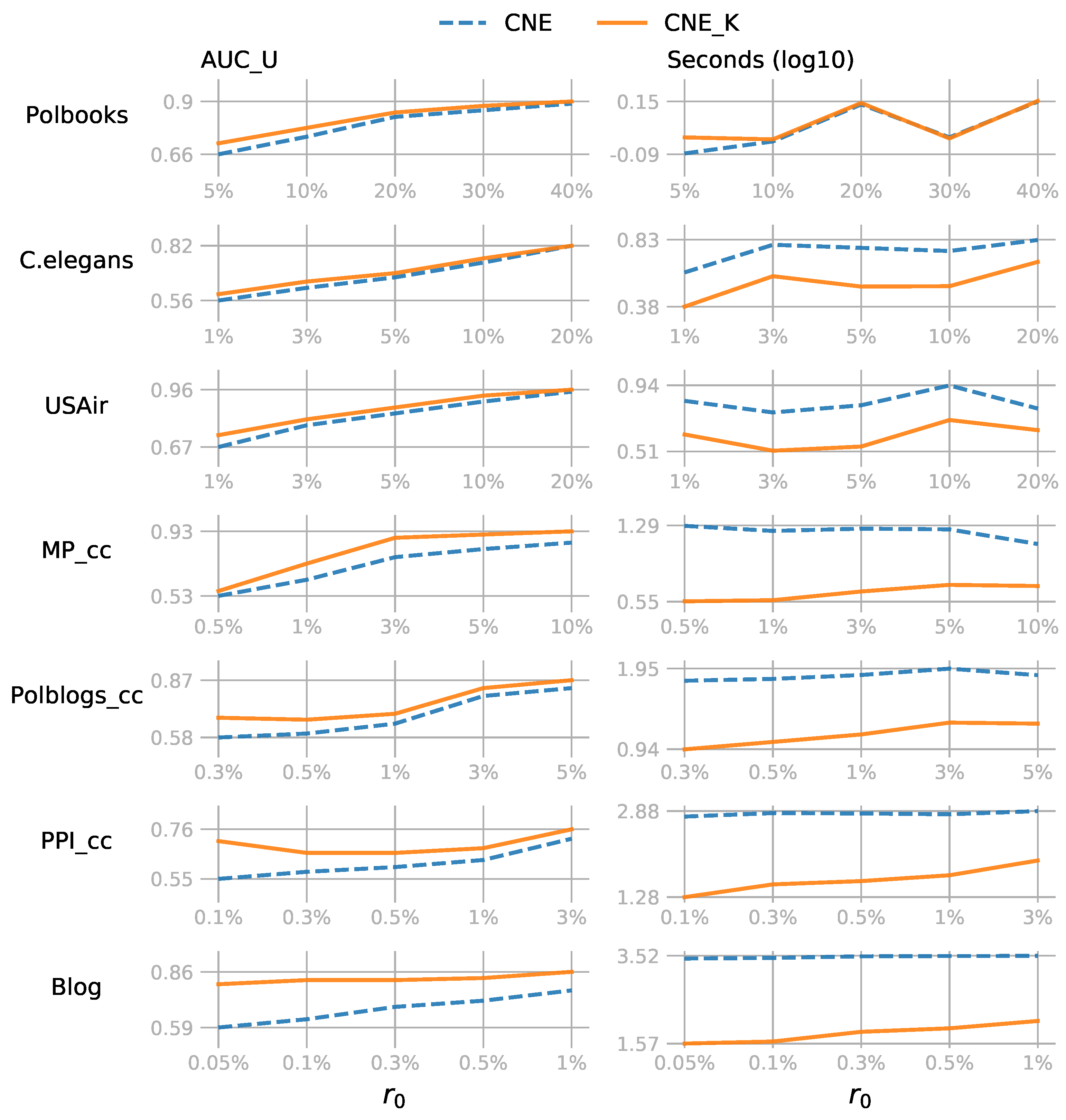
An important hypothesis underlying this work is that distinguishing an “observed unlinked” status of a node pair from an “unknown/unobserved” status, as opposed to treating both as absent, which is commonly performed, will enhance the performance of network embedding. We now empirically investigated this hypothesis by comparing CNE with its variant that performs partial network embedding: (1) the original CNE defined by its objective function in Equation (1), which does not make this distinction, and (2) the modified version that optimizes Equation (3), which we called CNE_K (i.e., CNE for the Knowns), which does make the distinction. Specifically, we compared the model fitting time and the link prediction accuracy for both:

• CNE: fit the entire network where the unobserved link status is treated as unlinked;
• CNE_K: fit the model only for the observed linked and unlinked node pairs.

Setup: To construct a PON, we first initialized the observed information by randomly sampling a node pair set $K_0=E\cup D$ that contained a proportion $r_0$ of the complete information. The complete information means the total number of links in the complete graph for a given number of nodes. For example, $r_0=10\%$ means that $10\%$ of the network link statuses are observed as either linked or unlinked: if the network has n nodes, $\left|K_0\right|=10\%\times \frac{n(n-1)}{2}$. The observed $K_0$ is guaranteed connected as this is a common assumption for network embedding methods. Then, we embedded the same PON using both CNE and CNE_K on a machine with an Intel Core i7 CPU 4.20 GHz and 32 GB RAM.

Results: From the results shown in Figure 2, we see that CNE_K was not only more time efficient, but also provided more accurate link predictions. The ratio $r_0$ of observed information varied for datasets because the larger the network, the more time consuming the computations are. The time differences for a small observed part were enough to highlight the time efficiency of CNE_K. The two measures examined were: AUC_U—the prediction AUC score for all unobserved node pairs $(i,j)\in U$ containing $1-r_0$ network information; and t(s)—the model fitting time in seconds. Both values are averaged—for each $r_0$ averaged over 10 different PONs and each PON with 10 different embeddings (i.e., CNE has local optima) for the first four datasets—while it is $5\times 5$ for the fifth and sixth and $3\times 3$ for the last dataset.

It is not surprising that the fitting time of CNE_K was almost always shorter than the original CNE as CNE_K only fits the observed information. One exception was the Polbooks network, on which both methods used similar amounts of time, because the network size was not large. However, as the network size increased, CNE_K showed increasing time efficiency. Especially for the Blog network: with $r_0=0.05\%$, CNE_K was 76 times faster than CNE. CNE_K thus enabled network embedding to scale more easily to large networks.

In addition to time efficiency, CNE_K always achieved a higher AUC than CNE, since CNE will try to model the absence of an edge even where there might actually be an (unobserved) edge. In other words, CNE was trained on data with a substantial amount of label noise: 0 labels (absent edge) that actually must be a 1 (present edge), while CNE_K only used those labels that were known to be correct. Partial network embedding for the knowns is especially useful in settings where only a small part of a large network is observed and the goal is to predict the unobserved links.

5.2. Qualitative Evaluation of ALPINE

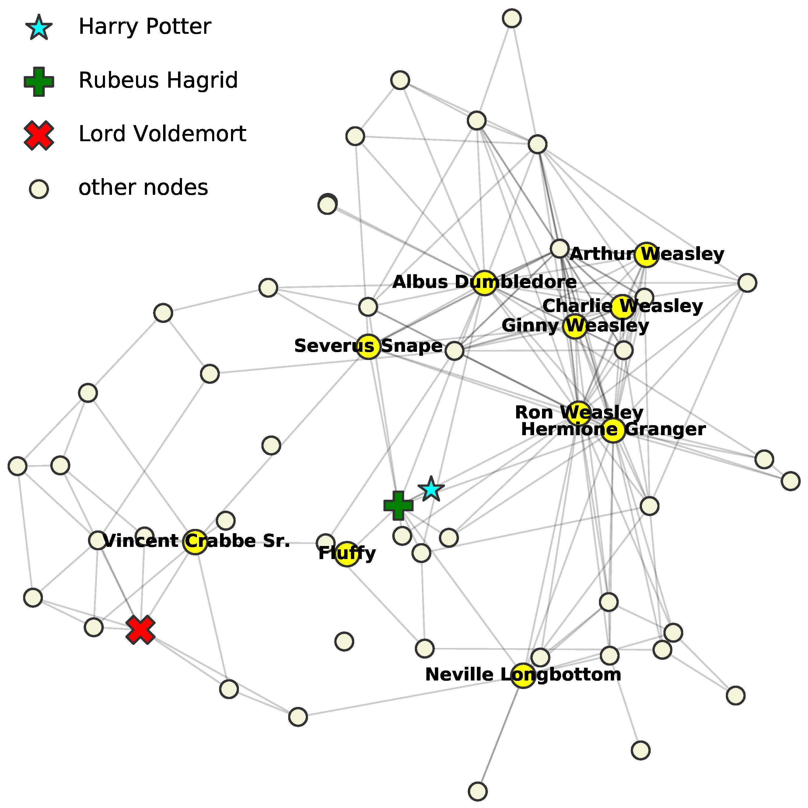
In Section 1, we used the Harry Potter network to illustrate the idea of ALPINE with three of our query strategies, which focused on predicting the unknown links for a target node—“Harry Potter”—who has very limited observed information to the rest of the network. Now, we complete this qualitative evaluation with the same setting for other strategies: page-rank., d-opt., and v-opt.; min-dis. was omitted as it approximates max-prob.

Table 3. Top 5 query selections for the other three strategies of ALPINE.

Strategy	Page-Rank.	d-opt.	v-opt.
1	Ron Weasley	Hermione Granger	Arthur Weasley
2	Albus Dumbledore	Ron Weasley	Fluffy
3	Hermione Granger	Albus Dumbledore	Charlie Weasley
4	Vincent Crabbe Sr.	Severus Snape	Albus Dumbledore
5	Neville Longbottom	Ginny Weasley	Ron Weasley

shows the top five suggestions, and the relevant characters are highlighted in Figure 3 with their names. Since CNE achieved different local optima, here, we used a different two-dimensional visualization to better display the names. All the suggestions were reasonable and could be explained from different perspectives, proving that ALPINE with those query strategies made sense qualitatively. Similar to max-deg. and max-prob., page-rank. and d-opt. had the same top three suggestions: Hermione, Ron, and Albus, which are essential allies of Harry. Knowing whether Harry is linked to them will give a clear big picture of his social relations. The results can further be analyzed according to the strategy definitions.

Strategy page-rank., as max-deg., aims to find out Harry’s relationships with the influencers—nodes that are observed to have many links. With this type of strategy, we learned which influencers Harry is close to, as well as his potential allies connecting to them; and conversely for his unlinked influencers.

The d-opt. strategy selects queries based on the parameter variance reduction. It implies that by knowing whether Harry is linked to the suggested nodes, the node embeddings will have a smaller variance, such that the entire embedding space is more stable, and thus, the link predictions are more reliable. For example, Severus, who ranks the fourth here (also the fourth with max-ent.), was not an obvious ally of Harry, but he helps secretly and is essential in shaping the network structure. The suggestions were considered uncertain and contributed to the reduction of the parameter variance.

The v-opt. strategy quantifies the informativeness of the unobserved link statuses by the amount of estimated prediction variance reduction they cause. It suggests that Harry’s relationships to the Weasley family are informative for minimizing the prediction variance for him. It makes sense as this family is well connected with Rubeus, who is Harry’s known ally, and also connects well with other nodes. As for Fluffy, it was observed to be connected only to Rubeus and unlinked to all other nodes except Harry. Knowing whether Fluffy and Harry are linked greatly reduced the variance on the prediction for the unobserved, because there was no other information for it.

We concluded that, intuitively, the query strategies resulted in expected behavior, although we caution against overinterpretation of this subjective qualitative evaluation. The next, quantitative, evaluation, provided an objective assessment of the merits of the query strategies, relative to passive learning, to each other, and to the single pre-existing method of which we we are aware.

5.3. Quantitative Evaluation of ALPINE

In the quantitative evaluation, we mainly wanted to compare the performance of different query strategies from Section 4 with passive learning, as well as with the state-of-the-art baseline method HALLP [9]. Passive learning is represented by the random strategy that uniformly selects node pairs from the pool. As for HALLP, we implemented its query strategy shown in Equation (2) (since the source code is not publicly available), and set $c_1$ and $c_2$ both to one. Note that, as we wanted to compare query strategies in the fairest possible way, the link prediction was performed using CNE_K also for HALLP.

Setup: As before, we constructed a PON by randomly initializing the observed node pair set $K_0$ with a given ratio $r_0$, while making sure $K_0$ was connected. Then, we applied ALPINE with different query strategies for a budget k and a step size s. More specifically, we investigated three representative different cases depending on the pool P and the target set T:

• $P=U$ and $T=U$: all the unobserved information was accessible, and we were interested in knowing all link statuses in U;
• $P\subset U$ and $T=U$: only part of U was accessible, and we still wanted to predict the entire U as accurately as possible;
• $P\subset U$, $T\subset U$, and $T\cap U=\varnothing$: only part of U was accessible, and we were interested in predicting a different set of unobserved link status that was inaccessible.

For all datasets, we investigated four values of $r_0$: $\left[3\%,10\%,30\%,80\%\right]$, to see how the percentage of the observed information affected the strategy performance. All quantitative experiments used a step size depending on the network size: $1\%$ of the network information. For a network with n nodes, it means that $s=1\%*\frac{n(n-1)}{2}$ unobserved candidate link statuses will be selected for querying in each iteration. Then, the budget k, pool size $\left|P\right|$, and target set size $\left|T\right|$ were multiples of s for different cases. The random strategy was a baseline for all three cases, while the HALLP strategy was only used in the first case because it was designed only for this setup.

Below, we first discuss our findings for each of the three cases on the five smallest datasets. After that, we discuss some results on the two larger networks for the most scalable query strategies only.

5.3.1. Case 1: $P=U$ and $T=U$

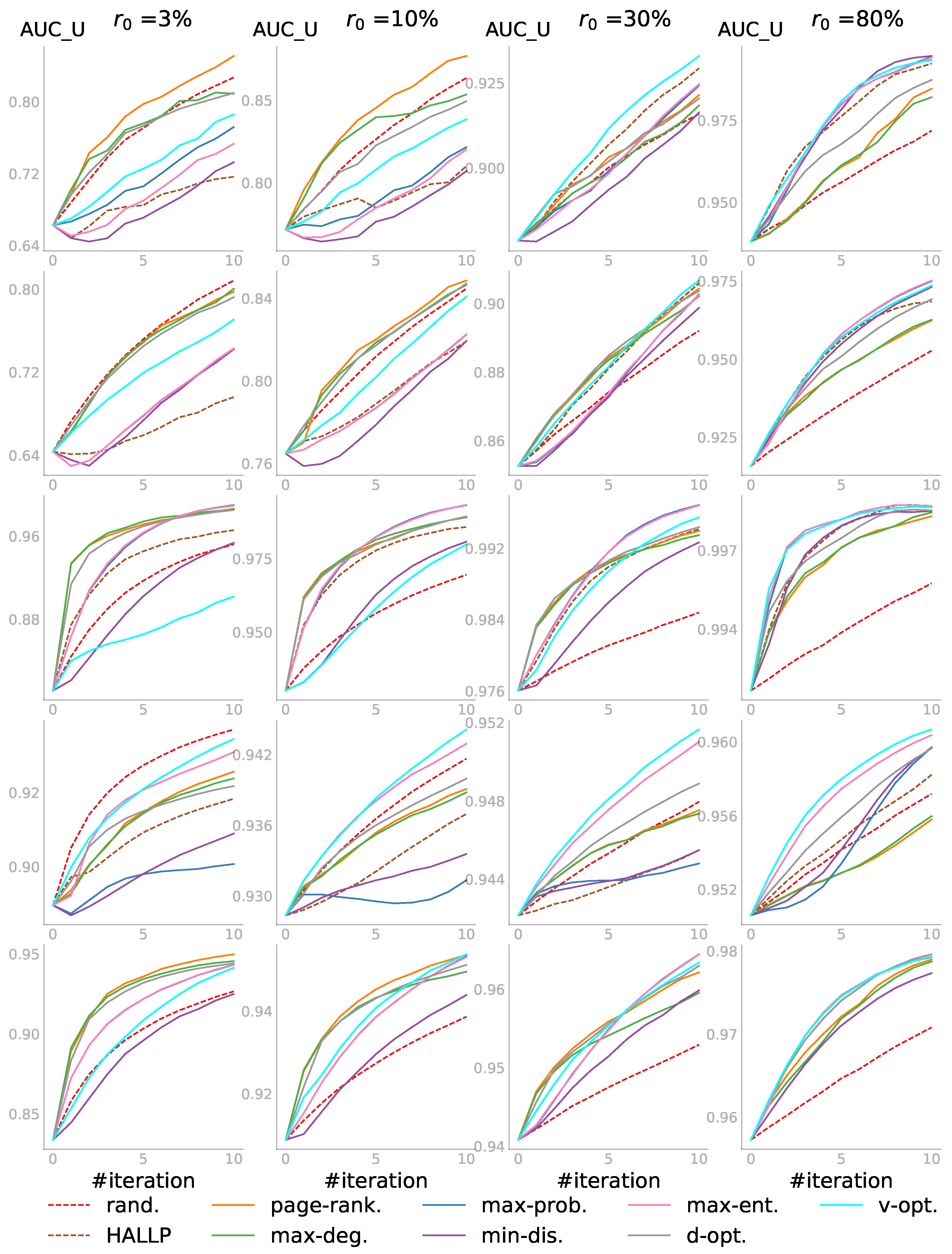
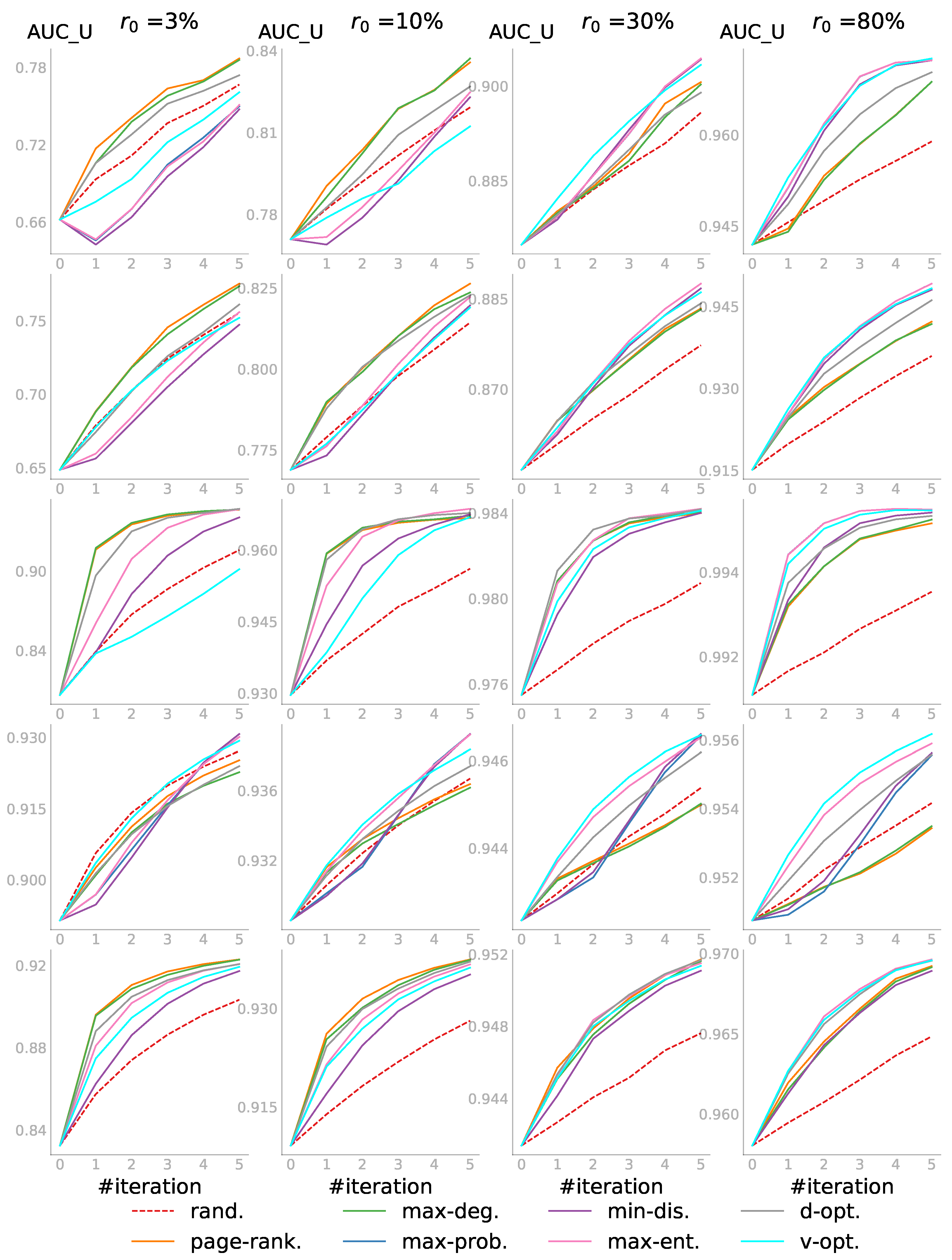
In the first case, we had the pool of all unobserved link statuses and wanted to predict all the unknowns. Shown in Figure 4 are the results, in which each row represents a dataset with its step size and each column corresponds to one $r_0$ value. For every individual subplot, the $AUC\_U$ is the AUC score for all the initially unobserved link statuses—those not included in $K_0$. The budget k was set to 10 steps, i.e., $k=10s$, resulting in 10 iterations. Iteration 0 was the initial performance before the active learning, so there were always $\frac{k}{s}+1$ scores. In other words, given the budget $k=10s$, even for $r_0=80\%$, we did not query the entire pool and reached only $90\%$ of the network information. The AUC scores were averaged over several different random PONs, and each PON defined by a $K_0$ was initialized with different random embeddings ($10\times 10$ for the first four networks and $5\times 5$ for the last and largest one). Each random strategy score was further averaged over three runs.

In general, the active learning strategies outperformed the rand. strategy. We saw that when the observed part was relatively small—$3\%$ or $10\%$— the degree-related strategies that did not depend on the embedding usually performed very well, and the random strategy was not always the worst. As more information was observed when $r_0$ increased (see the plots from the left to the right in each row), we did not only see that the active learning strategies, such as v-opt. and max-ent., began to dominate and passive learning became the worst, but also the increase of the starting $AUC\_U$. Zooming in to individual subplots, we saw that ALPINE boosted link prediction accuracy with far fewer queries for the active learning strategies, compared to passive learning. Overall, when the observed information was very limited, the embedding-independent strategies page-rank. and max-deg. outperformed the others; while for sufficiently enough information, v-opt. and max-ent. were the better choices. We speculated that this was the case as the embedding must be of sufficient quality for the embedding-dependent strategies to work, which requires a certain minimum amount of data. Worth noticing is that d-opt. showed similar performance across different values of $r_0$, which will be discussed further in Section 5.4.

As for the HALLP strategy, which aimed to query the most uncertain node-pairs and thus was similar in spirit to max-ent., the performance was very variable. In some cases, it performed quite well, as shown in the top right subplot, beating v-opt. in the first few iterations, while on the MP_cc network, it was one of the worst strategies. In addition to that, the runtime of HALLP was much longer than that of the other strategies; thus, some of the subplots do not have the HALLP result. The runtime analysis for one iteration of the query process on a server with an Intel Xeon Gold CPU 3.00 GHz and 256 GB RAM is shown in

Table 4. Runtime for one query in seconds—Case 1.

Data	Rand.	Page-Rank.	Max-Deg.	Max-Prob.	Min-Dis.	Max-Ent.	d-opt.	v-opt.	HALLP
Polbooks	0.001	0.031	0.008	0.004	0.027	0.004	0.093	0.482	12.33
C. elegans	0.005	0.108	0.042	0.028	0.18	0.029	0.675	5.469	148.4
USAir	0.006	0.134	0.052	0.035	0.231	0.036	0.881	7.309	232.6
MP_cc	0.016	0.707	0.16	0.117	0.693	0.125	2.746	28.90	1074
Polblogs_cc	0.092	1.153	0.707	0.675	3.264	0.709	12.31	226.0	12022

below. The results were averaged in the same way as in Figure 4 for the four values of $r_0$ and then further averaged over the $r_0$ values. Across different datasets, HALLP was by far the most computationally expensive strategy as it had to run two link predictors.

5.3.2. Case 2: $P\subset U$ and $T=U$

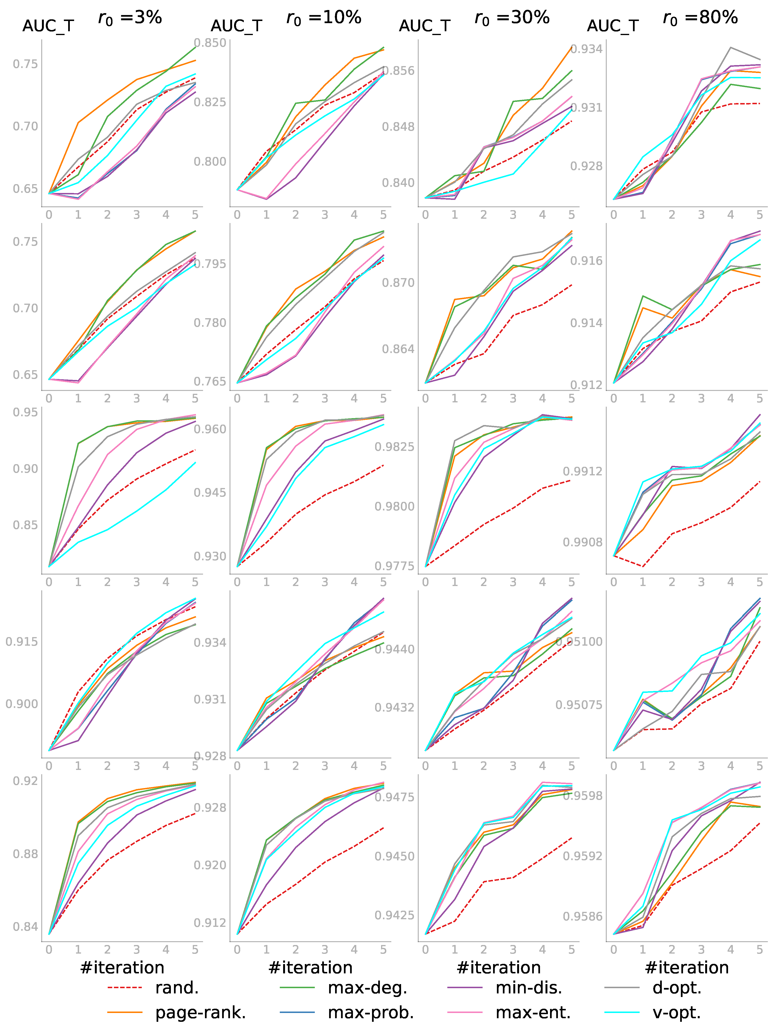
In the second case, we applied ALPINE with a smaller pool, while we were still interested in predicting all the unknown link statuses. The experiment setting was similar to the previous case, but the pool size $\left|P\right|$ was set to 10 times the step size—$10s$—and the budget $k=5s$, i.e., only five iterations were performed. The candidates in the pool were randomly sampled from the unobserved part for each PON in our experiments.

Figure 5 shows the results for this case. Compared to the first case, the $AUC\_U$ was lower for each individual subplot as the accessible information in the pool was more limited. The results confirmed again that all active learning strategies were better than passive learning, Shown more clearly in the last row in Figure 5 on the Polblogs_cc network is that the three strategies page-rank., max-deg., and d-opt. were the winning group for the first two $r_0$ values. However, in the third and fourth subplot in the same row, v-opt., max-ent., and d-opt. performed best. The d-opt. strategy stayed as one of the top strategies across different percentages of the observed information.

5.3.3. Case 3: $P\subset U$, $T\subset U$, and $T\cap U=\varnothing$

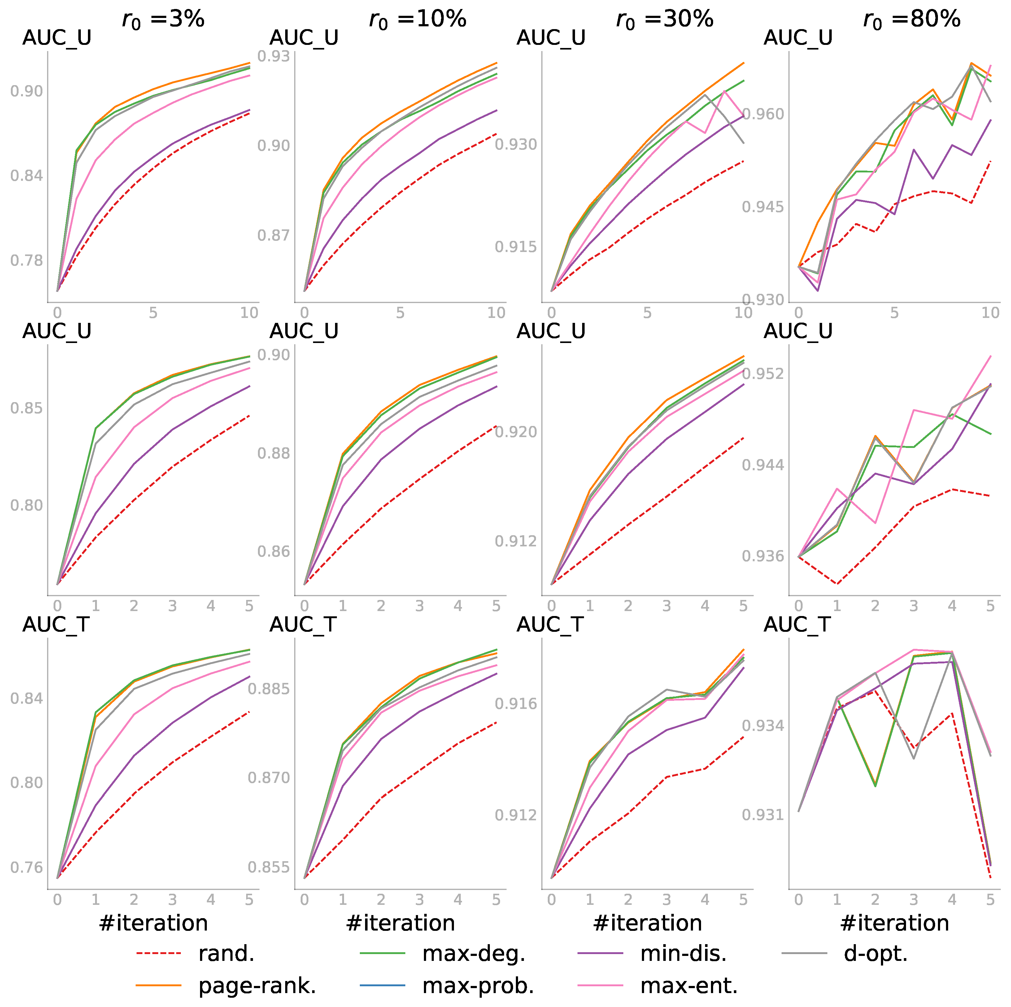
We imposed further constraints in the third case: not only the pool P of node pairs that could be queried was limited, but also the set T of target node-pairs for which we wanted to predict the status was limited. Moreover, both sets were not intersecting. As in the second case, the budget was set to $k=5s$ and $\left|P\right|=10s$. The target set size was now taken to be $\left|T\right|=5s$. Both P and T were sampled randomly from U before the querying started.

The results in Figure 6 confirmed again that active learning outperformed passive learning. One might expect v-opt. to perform the best in this case because it was the only strategy that explicitly considered T. Although it was shown to perform quite well in some subplots especially for the first iteration, the quality of the embedding affected its performance. Indeed, as we observed before, the reliability of all embedding-based strategies depended largely on how well the network was embedded, which became much better as $r_0$ increased.

Compared to the previous two cases, the results here were not as smooth even after averaging. The reason was that the score $AUC\_T$ depended not only on P, but also largely on T, which were both randomly sampled. Whether P contained candidate node pairs that were informative for T affected the score. Overall, the embedding-independent strategies—page-rank. and max-deg.—had the top performance when $r_0$ was small; and the embedding-based strategies became increasingly competitive if more information was observed.

5.3.4. Evaluations on Two Larger Networks

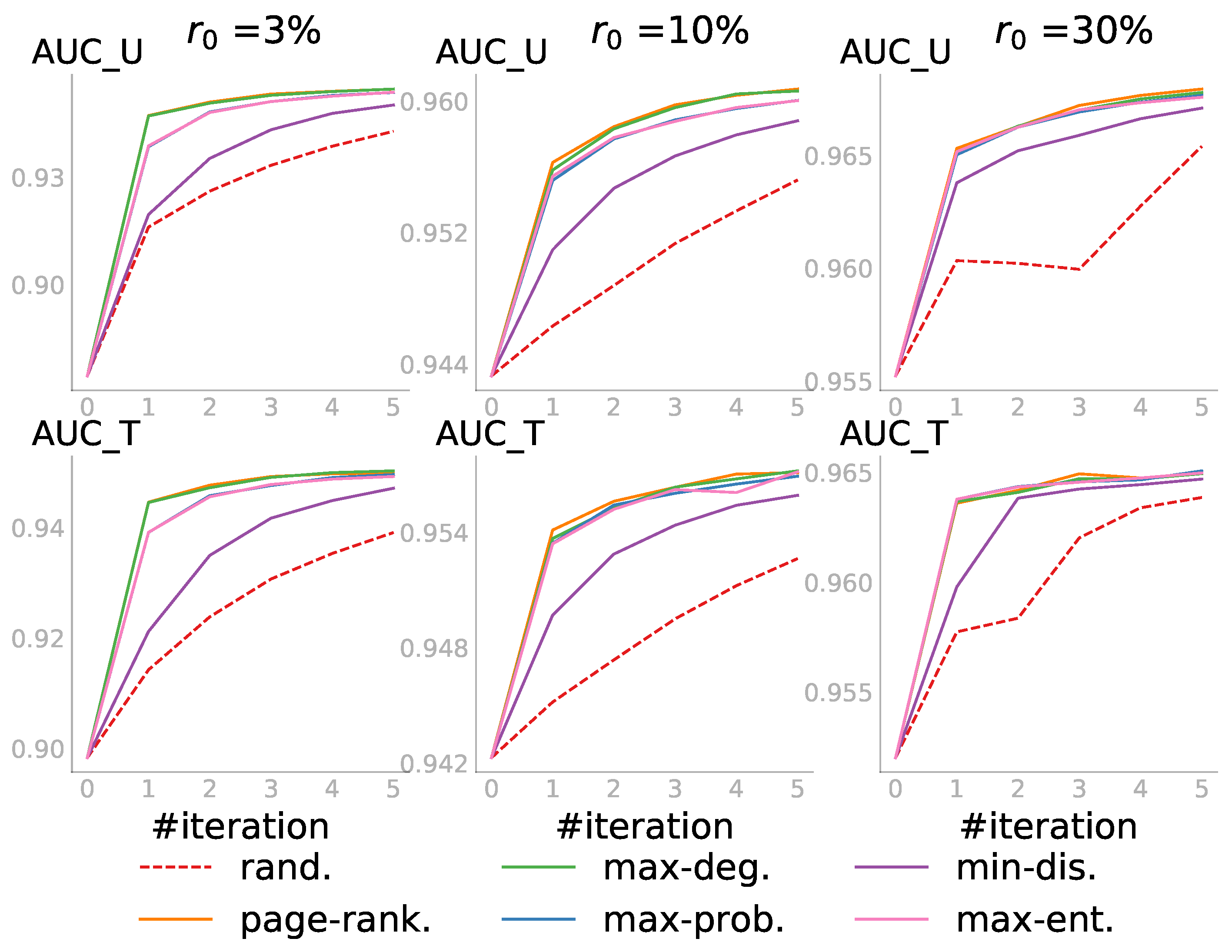
Finally, we conducted a quantitative evaluation on two larger networks: PPI_cc and Blog. The results are shown in Figure 7 and Figure 8 and confirmed the observations we made on the five smaller networks. Figure 7 shows the PPI_cc results for the three cases with seven query strategies, excluding v-opt. and HALLP, as they were computationally too expensive. The AUC scores were averaged over five sets of random initial $K_0$, P, and T, and each set with five initial embeddings. The last column looks bumpy since the score was already very high and small randomness in the embedding could cause a slight difference. Figure 8 shows the results for the second and third case with three values of $r_0$. Case 1 was omitted because embedding the Blog network with a large observed part was already quite expensive, and evaluating all the unobserved candidates when $r_0$ was small made it computationally too demanding.

5.4. Discussion

Our experiments showed that ALPINE in its general form can be adapted for various problem settings, and active learning performed consistently and substantially better than passive learning regardless of which of the investigated query strategies was applied. Now, we discuss how the strategies can be optimally applied based on our observations, with advice and insights that may help a practitioner select the best query strategy given the properties of the data and available computational resources.

Among the seven active learning query strategies we developed, page-rank. and max-deg. did not depend on the network embedding while the other five were embedding based. Thus, as with limited observed information, the network embedding might be of poor quality, in such cases, page-rank. and max-deg. were seen to outperform the others.

The embedding-based strategies began to dominate when more information was observed and the embedding quality improved. The max-ent. and v-opt. had the top performance, but d-opt. had a more stable high performance across different values of $r_0$. Based on those observations, we recommend a mixed strategy that starts from the degree-related and then switches to other embedding-based strategies.

The complexity of the utility computation depended on the sizes of P and T, as well as the network. Normally, the larger the pool, the more expensive the computations were, as we had to consider more candidate node pairs. All query strategies, including rand., required a similar computing time when given the same size of P. A notable exception is v-opt., which was computationally more expensive. Yet, if we had a sufficiently accurate network embedding model, e.g., see the last columns in Figure 4, Figure 5 and Figure 6, v-opt. was almost always the most accurate, especially for the first few iterations. Thus, when the cost of querying was high as compared to the cost of computations, v-opt. was preferable as soon as enough data were available such that the embedding was sufficiently accurate. If computational cost was a bottleneck though, max-ent. and d-opt. were computationally less expensive substitutes for v-opt., with comparable accuracies.

The experiments aimed to show how active learning, compared to passive learning, benefited the network embedding based link prediction, namely CNE. Therefore, following the line of research in active learning, we restricted our baselines to only the random and the state-of-the-art active learning strategies for link prediction [7,9,14,25]. However, it would also be interesting to compare ALPINE with CNE against other types of link prediction methods to gain more insights. For example, a comparison of our work with a state-of-the-art link prediction approach (e.g., SEAL [45] according to [46,47]) could be used to show whether the differentiation between the unknown and the unlinked status together with active learning would improve the link prediction accuracy in general. Note that this type of comparison can be biased as we had three types of link statuses, while other link prediction methods usually have only two. There are also other network embedding methods that can be used in combination with the ALPINE framework; thus the comparison among CNE and other base models can be considered. That leaves many possible opportunities for research to be built on this work.

6. Conclusions

Link prediction is an important task in network analysis, tackled increasingly using network embeddings. It is particularly important in partially observed networks, where finding out whether a node pair is linked is time consuming or costly, such that for a large number of node pairs, it is not known if they are linked. We proposed to make use of active learning in this setting and studied the problem of active learning for link prediction using network embedding in this paper.

More specifically, we proposed the ALPINE framework, a method that actively learns to embed partially observed networks to achieve better link predictions, by querying the labels of the most informative unobserved link statuses. We developed several utility functions for ALPINE to quantify the utility of a node pair: some heuristically motivated and some derived as variance reduction methods based on D-optimality and V-optimality from optimal experimental design.

We implemented ALPINE in combination with Conditional Network Embedding (CNE). To accomplish this, we first adapted CNE to work for partially observed networks. Through experimental investigation, we found that this modified version of CNE was not only more time efficient, but also more accurate for link prediction—an important side-result of the present paper.

We then empirically evaluated the performance of the utility functions we developed for ALPINE, both qualitatively and quantitatively, providing insights into the merits of ALPINE and advice for practitioners on how to optimally apply this method to different problem settings.

More broadly, the application of active learning to the link prediction problem in general, which is usually for partially observed networks, could help us to build more realistic and practical methods. Taking this work as a starting point, we see interesting future directions, including the investigation of a mixed strategy, batch mode active learning for ALPINE, and the application of ALPINE to the cold-start problem in recommender systems. Meanwhile, a thorough comparison of ALPINE with CNE against general link prediction methods, as well as the choice of the base network embedding model to be used with the ALPINE framework remain to be further investigated.

References

- Cui, P.; Wang, X.; Pei, J.; Zhu, W. A Survey on Network Embedding. IEEE Trans. Knowl. Data Eng. 2019, 31, 833–852. [Google Scholar] [CrossRef] [Green Version]
- Liben-Nowell, D.; Kleinberg, J. The Link-Prediction Problem for Social Networks. J. Am. Soc. Inf. Sci. Technol. 2007, 58, 1019–1031. [Google Scholar] [CrossRef] [Green Version]
- Martínez, V.; Berzal, F.; Cubero, J.C. A Survey of Link Prediction in Complex Networks. ACM Comput. Surv. 2016, 49, 1–33. [Google Scholar] [CrossRef]
- Mara, A.C.; Lijffijt, J.; De Bie, T. Benchmarking Network Embedding Models for Link Prediction: Are We Making Progress? In Proceedings of the 7th IEEE International Conference on Data Science and Advanced Analytics, Sydney, Australia, 6–9 October 2020; pp. 138–147. [Google Scholar]
- Zhao, Y.; Wu, Y.J.; Levina, E.; Zhu, J. Link Prediction for Partially Observed Networks. J. Comput. Graph. Stat. 2017, 26, 725–733. [Google Scholar] [CrossRef] [Green Version]
- Cesa-Bianchi, N.; Gentile, C.; Vitale, F.; Zappella, G. A Linear Time Active Learning Algorithm for Link Classification. In Proceedings of the 26th International Conference on Neural Information Processing Systems, Lake Tahoe, NV, USA, 3–6 December 2012; Volume 25. [Google Scholar]
- Ostapuk, N.; Yang, J.; Cudré-Mauroux, P. ActiveLink: Deep Active Learning for Link Prediction in Knowledge Graphs. In Proceedings of the 2019 World Wide Web Conference, San Francisco, CA, USA, 13–17 May 2019; pp. 1398–1408. [Google Scholar]
- Jia, J.; Schaub, M.T.; Segarra, S.; Benson, A.R. Graph-based Semi-Supervised & Active Learning for Edge Flows. In Proceedings of the 25th ACM SIGKDD International Conference on Knowledge Discovery and Data Mining, Anchorage, AK, USA, 4–8 August 2019; pp. 761–771. [Google Scholar]
- Chen, K.J.; Han, J.; Li, Y. HALLP: A Hybrid Active Learning Approach to Link Prediction Task. J. Comput. 2014, 9, 551–556. [Google Scholar] [CrossRef]
- Kang, B.; Lijffijt, J.; De Bie, T. Conditional Network Embeddings. In Proceedings of the 7th International Conference on Learning Representations, New Orleans, LA, USA, 6–9 May 2019. [Google Scholar]
- Evans, C.; Friedman, J.; Karakus, E.; Pandey, J. PotterVerse. 2014. Available online: https://github.com/efekarakus/potter-network (accessed on 31 March 2019).
- Brinker, K. Incorporating Diversity in Active Learning with Support Vector Machines. In Proceedings of the 20th International Conference on Machine Learning, Washington, DC, USA, 21–24 August 2003; pp. 59–66. [Google Scholar]
- Cai, H.; Zheng, V.W.; Chang, K.C.C. Active Learning for Graph Embedding. arXiv 2017, arXiv:1705.05085. [Google Scholar]
- Settles, B. Active Learning Literature Survey; Technical Report; University of Wisconsin: Madison, WI, USA, 2009. [Google Scholar]
- Atkinson, A.; Donev, A.; Tobias, R. Optimum Experimental Designs, with SAS; Oxford University Press: Oxford, UK, 2007. [Google Scholar]
- Cohn, D.A.; Ghahramani, Z.; Jordan, M.I. Active Learning with Statistical Models. J. Artif. Intell. Res. 1996, 4, 129–145. [Google Scholar] [CrossRef]
- Zhang, T.; Oles, F.J. A Probability Analysis on the Value of Unlabeled Data for Classification Problems. In Proceedings of the 17th International Conference on Machine Learning, Stanford, CA, USA, 29 June–2 July 2000; pp. 1191–1198. [Google Scholar]
- Perozzi, B.; Al-Rfou, R.; Skiena, S. DeepWalk: Online Learning of Social Representations. In Proceedings of the 20th ACM SIGKDD International Conference on Knowledge Discovery and Data Mining, New York, NY, USA, 24–27 August 2014; pp. 701–710. [Google Scholar]
- Grover, A.; Leskovec, J. node2vec: Scalable Feature Learning for Networks. In Proceedings of the 22nd ACM SIGKDD International Conference on Knowledge Discovery and Data Mining, San Francisco, CA, USA, 13–17 August 2016; pp. 855–864. [Google Scholar]
- Kipf, T.N.; Welling, M. Semi-Supervised Classification with Graph Convolutional Networks. In Proceedings of the 5th International Conference on Learning Representations, Toulon, France, 24–26 April 2017. [Google Scholar]
- Chen, X.; Yu, G.; Wang, J.; Domeniconi, C.; Li, Z.; Zhang, X. ActiveHNE: Active Heterogeneous Network Embedding. In Proceedings of the 28th International Joint Conference on Artificial Intelligence, Macao, China, 10–16 August 2019; pp. 2123–2129. [Google Scholar]
- Yang, Z.; Cohen, W.; Salakhudinov, R. Revisiting Semi-Supervised Learning with Graph Embeddings. In Proceedings of the 33rd International Conference on Machine Learning, New York, NY, USA, 19–24 June 2016; pp. 40–48. [Google Scholar]
- Aggarwal, C.C.; Kong, X.; Gu, Q.; Han, J.; Philip, S.Y. Active Learning: A Survey. In Data Classification: Algorithms and Applications; CRC Press: Boca Raton, FL, USA, 2014; pp. 571–605. [Google Scholar]
- Kong, X.; Fan, W.; Yu, P.S. Dual Active Feature and Sample Selection for Graph Classification. In Proceedings of the 17th ACM SIGKDD International Conference on Knowledge Discovery and Data Mining, San Diego, CA, USA, 21–24 August 2011; pp. 654–662. [Google Scholar]
- Bilgic, M.; Mihalkova, L.; Getoor, L. Active Learning for Networked Data. In Proceedings of the 27th International Conference on Machine Learning, Haifa, Israel, 21–24 June 2010; pp. 79–86. [Google Scholar]
- Cesa-Bianchi, N.; Gentile, C.; Vitale, F.; Zappella, G. Active Learning on Trees and Graphs. arXiv 2013, arXiv:1301.5112. [Google Scholar]
- Guillory, A.; Bilmes, J.A. Label Selection on Graphs. In Proceedings of the 23rd International Conference on Neural Information Processing Systems, Vancouver, BC, Canada, 7–10 December 2009; Volume 22. [Google Scholar]
- Yang, Z.; Tang, J.; Zhang, Y. Active Learning for Streaming Networked Data. In Proceedings of the 23rd ACM International Conference on Information and Knowledge Management, Shanghai, China, 3–7 November 2014; pp. 1129–1138. [Google Scholar]
- Cortes, C.; Vapnik, V. Support-Vector Networks. Mach. Learn. 1995, 20, 273–297. [Google Scholar] [CrossRef]
- Clauset, A.; Moore, C.; Newman, M.E. Hierarchical structure and the prediction of missing links in networks. Nature 2008, 453, 98–101. [Google Scholar] [CrossRef] [PubMed]
- Page, L.; Brin, S.; Motwani, R.; Winograd, T. The PageRank Citation Ranking: Bringing Order to the Web; Technical Report; Stanford InfoLab: Stanford, CA, USA, 1999. [Google Scholar]
- Smith, K. On the Standard Deviations of Adjusted and Interpolated Values of an Observed Polynomial Function and its Constants and the Guidance they give Towards a Proper Choice of the Distribution of Observations. Biometrika 1918, 12, 1–85. [Google Scholar] [CrossRef] [Green Version]
- Welch, W.J. Computer-Aided Design of Experiments for Response Estimation. Technometrics 1984, 26, 217–224. [Google Scholar] [CrossRef]
- Liu, S.; Neudecker, H. A V-optimal design for Scheffé’s polynomial model. Stat. Probab. Lett. 1995, 23, 253–258. [Google Scholar] [CrossRef]
- Lehmann, E.L.; Casella, G. Theory of Point Estimation; Springer Science & Business Media: Berlin/Heidelberg, Germany, 2006. [Google Scholar]
- Rao, C.R. Information and the Accuracy Attainable in the Estimation of Statistical Parameters. In Breakthroughs in Statistics; Springer: Berlin/Heidelberg, Germany, 1992; pp. 235–247. [Google Scholar]
- Efron, B.; Hinkley, D.V. Assessing the Accuracy of the Maximum Likelihood Estimator: Observed Versus Expected Fisher Information. Biometrika 1978, 65, 457–483. [Google Scholar] [CrossRef]
- Harville, D.A. Matrix Algebra From a Statistician’s Perspective. Technometrics 1998, 40, 164. [Google Scholar] [CrossRef]
- Sherman, J.; Morrison, W.J. Adjustment of an Inverse Matrix Corresponding to a Change in One Element of a Given Matrix. Ann. Math. Stat. 1950, 21, 124–127. [Google Scholar] [CrossRef]
- Adamic, L.A.; Glance, N. The Political Blogosphere and the 2004 U.S. Election: Divided They Blog. In Proceedings of the 3rd International Workshop on Link Discovery, Chicago, IL, USA, 21–25 August 2005; pp. 36–43. [Google Scholar]
- Watts, D.J.; Strogatz, S.H. Collective dynamics of ’small-world’ networks. Nature 1998, 393, 440–442. [Google Scholar] [CrossRef] [PubMed]
- Handcock, M.S.; Hunter, D.R.; Butts, C.T.; Goodreau, S.M.; Morris, M. statnet: An R Package for the Statistical Modeling of Social Networks. 2003. Available online: http://www.Csde.Washington.Edu/Statnet (accessed on 22 November 2018).
- Breitkreutz, B.J.; Stark, C.; Reguly, T.; Boucher, L.; Breitkreutz, A.; Livstone, M.; Oughtred, R.; Lackner, D.H.; Bähler, J.; Wood, V.; et al. The BioGRID Interaction Database: 2008 update. Nucleic Acids Res. 2007, 36, D637–D640. [Google Scholar] [CrossRef] [PubMed] [Green Version]
- Zafarani, R.; Liu, H. Social Computing Data Repository at ASU. 2009. Available online: http://socialcomputing.asu.edu (accessed on 22 November 2018).
- Zhang, M.; Chen, Y. Link Prediction Based on Graph Neural Networks. In Proceedings of the 32nd International Conference on Neural Information Processing Systems, Montréal, QC, Canada, 3–8 December 2018; Volume 31. [Google Scholar]
- Li, P.; Wang, Y.; Wang, H.; Leskovec, J. Distance Encoding: Design Provably More Powerful Neural Networks for Graph Representation Learning. In Proceedings of the 34th International Conference on Neural Information Processing Systems, virtual, 6–12 December 2020; Volume 33, pp. 4465–4478. [Google Scholar]
- Lin, W.; Ji, S.; Li, B. Adversarial Attacks on Link Prediction Algorithms Based on Graph Neural Networks. In Proceedings of the 15th ACM Asia Conference on Computer and Communications Security, Taipei, Taiwan, 5–9 October 2020; pp. 370–380. [Google Scholar]
Figure 1.
Harry Potter network with suggestions from Table 1 highlighted.
Figure 2.
Comparison of CNE_K and CNE.
Figure 3.
Harry Potter network with suggestions from Table 3 highlighted.
Figure 4.
ALPINE: and . Row 1: Polbooks (); Row 2: C. elegans (); Row 3: USAir (); Row 4: MP_cc (); Row 5: Polblogs_cc ().
Figure 5.
ALPINE— and . Row 1: Polbooks (); Row 2: C. elegans (); Row 3: USAir (); Row 4: MP_cc (); Row 5: Polblogs_cc ().
Figure 6.
ALPINE: , , and . Row 1: Polbooks (); Row 2: C. elegans (); Row 3: USAir (); Row 4: MP_cc (); Row 5: Polblogs_cc ().
Figure 7.
ALPINE on PPI_cc with . Row 1: Case 1; Row 2: Case 2; Row 3: Case 3.
Figure 8.
ALPINE on Blog with s = 531,635. Row 1: Case 2; Row 2: Case 3.