Array Gain of a Linear Array in an Ocean Waveguide

Abstract

Array gain is investigated based on the acoustic channel characteristics manifested by the fluctuant transmission loss and decrease in the acoustic channel spatial coherence. An analytical expression is derived as the summation of the products of the acoustic channel correlation coefficients and root-mean-square pressures. The formula provides insight into the physical mechanisms of the gain degradation in the ocean waveguide. Furthermore, this formula provides a new method to study array gain in the ocean waveguide from underwater acoustic field. The obtained expression is a more general formula that is applicable to shallow water, deep sea, and continental slope, with the traditional methods as a special case. Numerical results show that the array gain calculated by previous formulas are generally overestimated, caused by ignoring the effect of transmission loss fluctuation.

1. Introduction

Sonar, no matter if passive or active, often uses array to improve the performance of communication, detection or localization depending on the end use. The improvement can be measured by array gain (AG). Array gain is defined as an improvement in the signal-to-noise ratio (SNR) obtained for an array output compared to that for a single element [1]. It is one of the most important measures of the sonar system performance which is subjected to the inhomogeneous waveguide. For the AG of a linear array, critical questions are usually posed as: How much improvement will be obtained with an array in a specific ocean waveguide? What is the length of the designed array that can ensure that the array still provides the added gain? Before addressing these questions, one should find out the mechanism of the gain affected by the ocean waveguide. Under ideal assumptions, i.e., the noise is uncorrelated, and the signal is a perfect plane wave (far field), AG can reach its ideal value $10{\log }_{10}M$, where $M$ is the number of elements in the array [2]. However, both assumptions are violated in practical sonar applications, where a waveguide must be considered. The real ocean waveguide manifests as a complex acoustic channel with spatial and temporal fluctuations that are caused mainly by the rough sea surface, the sound speed profile (SSP) and the seabed topography [3]. These factors cause the wave-front to undergo distortion and the signals to show amplitude/phase fluctuations varying across different elements [4]. This outcome ultimately leads to the practical AG lower than the ideal value [5], especially for a long-towed array [6,7]. Nevertheless, both the decline in AG and its underlying mechanism have not been explicitly explored, due to the lack of research efforts to the study of the acoustic channel characteristics. A precise formula is needed to describe the effect of the acoustic channels on AG.

Previous research has derived the expression for AG when the signal phase fluctuations are governed by a Gaussian joint-probability density function [8,9,10]. In the ocean waveguide, the fluctuations of the acoustic channel transfer functions that lead to the degradation of the coherence [11,12] determine the signal phase fluctuations. Urick calculated AG using the correlation coefficients of the signal and noise between all pairs of elements. Based on the Urick formula, Cox [13] and Green [14] have derived the expression for AG in the uncorrelated noise, under the assumptions that the signal coherence decreases exponentially or linearly with the element separation, respectively. However, the signal coherence is determined by the waveguide that has uncertain change and the coherence lengths are different in shallow water or deep sea [15,16,17]. Furthermore, the formulas cannot predict the effect of acoustic channels on AG. In practice, different mechanisms give rise to the influence of the waveguide on the signal and the noise. In this case, AG can be divided into the array signal gain and noise gain, which has been used to study the AG of a passive vertical array [18]. In shallow water, AG can be expressed in terms of discrete normal modes [19], providing insight into the problem of the AG affected by the range-independent waveguide. However, the modes are coupled in a range-dependent waveguide, and the analyses based on the normal mode have not yet been developed for this case. A general formula of AG for a linear array in the ocean waveguide is derived in this paper based on the acoustic channel spatial coherence and the propagation losses. The physical problems involved in underwater acoustic signal processing that affect AG are investigated from the acoustic channel.

The paper has the following organization. The traditional method presented by Urick [1] is outlined in Section 2. Then, the analytical expression of AG in an isotropic noise field is derived in Section 3. Some useful results are provided and are verified by numerical simulations in Section 4. Finally, we provide a short summary and draw the conclusion in Section 5.

2. Array Gain for Plane Wave

The array gain for an arbitrary array is defined as [2]:

$$AG=\frac{SN{R}_{\mathrm{array}}}{SN{R}_{\mathrm{hyp}}},$$

(1)

where $SN{R}_{\mathrm{array}}$ is the SNR at the array output, and $SN{R}_{\mathrm{hyp}}$ is that at a single element of the array. The traditional formula given by Urick calculates AG as:

$$A{G}_{\mathrm{U}}={\displaystyle \sum _{i=1}^M{\displaystyle \sum _{k=1}^M{\left({\rho }_s\right)}_{ik}}}/{\displaystyle \sum _{i=1}^M{\displaystyle \sum _{k=1}^M{\left({\rho }_n\right)}_{ik}}},$$

(2)

where ${\left({\rho }_s\right)}_{ik}$ and ${\left({\rho }_n\right)}_{ik}$ are the signal and noise correlation coefficients between the $i$th and $k$th elements, respectively. $M$ is the number of elements. The subscript “U” indicates that this formula was given by Urick. If the ambient noise is uncorrelated, $A{G}_{\mathrm{U}}=\frac{1}{M}{\displaystyle \sum _{i=1}^M{\displaystyle \sum _{k=1}^M{\left({\rho }_s\right)}_{ik}}}$. $A{G}_{\mathrm{U}}$ can be only applied to the scenarios where both the signal powers and the noise powers are equal at their respective elements. However, this is not true in the real ocean as: (1) the propagation losses are not equal, and this inequality is more pronounced in the transition area between the shadow zone and the high intensity zone; (2) the noise power distribution is depth-dependent, particularly in deep sea [20]. In addition, Equation (2) does not take into account the effect of the ocean waveguide on the array performance. In the following, a theoretical formula for AG is derived in terms of the spatial-coherence of the acoustic channels and propagation losses that can help to interpret the degradation of AG caused by the acoustic channel fluctuation.

3. Array Gain in the Ocean Waveguide

In a real ocean environment, the elements of the array will have different outputs. We take the average of the SNRs at all the elements as the “single hydrophone” reference required in the definition in Equation (1). Moreover, the ocean waveguide has different effects on the signal field and the noise field, and the influence of the array processing on signal and noise should be considered separately. The ratio of the signal powers of the array output ($S_{\mathrm{array}}$) and the average powers ($S_{\mathrm{avg}}$) is defined as the array signal gain, denoted by $asg$. Similarly, the ratio of the noise powers of the array output ($N_{\mathrm{array}}$) and the average powers ($N_{\mathrm{avg}}$) is defined as the array noise gain, denoted by $ang$. Then, AG can be rewritten as:

$$A{G}_{\mathrm{W}}=\frac{SN{R}_{\mathrm{array}}}{SN{R}_{\mathrm{avg}}}=\frac{{\left(S/N\right)}_{\mathrm{array}}}{{\left(S/N\right)}_{\mathrm{avg}}}=\frac{S_{\mathrm{array}}}{S_{\mathrm{avg}}}/\frac{N_{\mathrm{array}}}{N_{\mathrm{avg}}}=\frac{asg}{ang},$$

(3)

where $SN{R}_{\mathrm{avg}}$ is the average SNR at all the elements.

For a short duration pulse, the acoustic channel can be regarded as linear time-invariant and characterized by the transfer function in the frequency domain. We assume that the array receives a narrow-band signal with a frequency band $\left[f_{\mathrm{L}},f_{\mathrm{H}}\right]$. The signal in the frequency domain at the $i$th element can be described as:

$$X_i(f)=S(f)H_i(f),$$

(4)

where $S\left(f\right)$ is the source spectrum, and $H_i\left(f\right)$ is the acoustic channel transfer function (or the Green’s function) between the source and the $i$th element, at frequency $f$. According to Parseval’s theorem, the signal energy on the $i$th element is given by:

$$E_i={\displaystyle {\int }_{-\infty }^{\infty }{\left|X_i(f)\right|}^2}df={\displaystyle {\int }_{-\infty }^{\infty }{\left|S(f)H_i(f)\right|}^2}df.$$

(5)

Dividing the signal band into a number of subbands, and assuming the transfer function to be constant in each subband, the integral in Equation (5) can be converted into a summation. Further, the power of the signal on the $i$th element can be rewritten as:

$$P_i=\frac{1}{T_s}{\displaystyle {\int }_{f_L}^{f_H}{\left|S(f)H_i(f)\right|}^2}df=\frac{{\left|S(f)\right|}^2}{T_s}{\displaystyle \sum _{b=1}^B{\left|H_i(f_b)\right|}^2},$$

(6)

where $T_s$ is the duration of the signal, and $B$ is the number of frequency bins in $\left[f_{\mathrm{L}},f_{\mathrm{H}}\right]$. $\left|H_i(f)\right|$ is the amplitude of the transfer function that takes the pressure at 1 m away from the source as the reference, which also denotes the pressure at the $i$th element. Denoting $p_i$ as the mean square of the pressure at the $i$th element:

$$p_i=\frac{1}{B}{\displaystyle \sum _{b=1}^B{\left|H_i(f_b)\right|}^2},$$

(7)

the average transmission loss (ATL) (averaged over the frequencies) is:

$${\mathrm{ATL}}_i{=-10\log }_{10}{p}_i,$$

(8)

and the average signal power $S_{\mathrm{avg}}$ of all elements is:

$$S_{\mathrm{avg}}=\frac{1}{M}{\displaystyle \sum _{i=1}^M{P}_i}=\frac{B{\left|S(f)\right|}^2}{T_{s}M}{\displaystyle \sum _{i=1}^M{p}_i}.$$

(9)

Denoting $h\triangleq {\left[\sqrt{p_1},\sqrt{p_2},\cdots ,\sqrt{p_M}\right]}^{\mathrm{T}}$, with the superscript “T” representing the transpose operation, Equation (9) can be written in a compact form as:

$$S_{\mathrm{avg}}=\frac{B{\left|S(f)\right|}^2}{T_{s}M}{‖h‖}_2^2,$$

(10)

where “${‖·‖}_2$” denotes the 2-norm of a vector.

The signal power at the array output after weighting is:

$$S_{\mathrm{array}}=\frac{1}{T_s}{\displaystyle {\int }_{f_L}^{f_H}{\left|{\displaystyle \sum _{i=1}^M{w}_i{X}_i(f)}\right|}^2}df=\frac{{\left|S(f)\right|}^2}{T_s}{\displaystyle \sum _{i=1}^M{\displaystyle \sum _{k=1}^M{\displaystyle {\int }_{f_L}^{f_H}{w}_i{H}_i(f)H_k{(f)}^{*}{w}_k{}^{*}}}}df,$$

(11)

where $w_i$ is the weighting coefficient at the $i$th element using to compensate for the phase difference between acoustic channels, and the superscript “*” denotes the complex conjugate operation. We define the spatial correlation coefficient of the acoustic channels $i$ and $k$ as:

$${\rho }_{ik}=\frac{\mathrm{Re}\left[{\displaystyle {\int }_{f_L}^{f_H}{H}_i(f)H_k{(f)}^{*}{e}^{j2\pi f\tau }df}\right]}{\sqrt{{\displaystyle {\int }_{f_L}^{f_H}{\left|H_i(f)\right|}^{2}df}}\sqrt{{\displaystyle {\int }_{f_L}^{f_H}{\left|H_k(f)\right|}^{2}df}}},$$

(12)

where $2\pi f\tau$ is the phase-shift that can maximize ${\rho }_{ik}$. The correlation coefficient matrix is then constructed as:

$$\rho =\left[\begin{array}{cccc}{\rho }_{11}& {\rho }_{12}& \cdots & {\rho }_{1M}\\ {\rho }_{21}& {\rho }_{22}& \cdots & {\rho }_{2M}\\ ⋮& ⋮& \ddots & ⋮\\ {\rho }_{M1}& {\rho }_{M2}& \dots & {\rho }_{MM}\end{array}\right].$$

(13)

We assume that the phase difference between the weights at the $i$th and the $k$th elements equal to $2\pi f\tau$ (maximize ${\rho }_{ik}$). When the uniform amplitude weighting (i.e., $\left|w_i\right|=1/M$) is applied, Equation (11) can be compacted by substituting Equations (12) and (13) into Equation (11), and after converting the integral to the summation, we obtain:

$$S_{\mathrm{array}}=\frac{B{\left|S(f)\right|}^2{h}^{\mathrm{T}}\rho h}{M^2{T}_s}.$$

(14)

The weighting amplitude has a slight influence on AG for a linear beamformer [21]. Hence, we are only concerned with the uniform amplitude weighting in the subsequent research.

According to Equations (10) and (14), the array signal gain can be obtained as:

$$asg=\frac{S_{\mathrm{array}}}{S_{\mathrm{avg}}}=\frac{h^{\mathrm{T}}\rho h}{M{‖h‖}_2^2}.$$

(15)

For an equal inter-element spacing $d$ in an isotropic ambient noise environment, $ang$ has been derived as [18]:

$$ang={\displaystyle \sum _{i=1}^M{w}_i{}^2}+2{\displaystyle \sum _{i=1}^{M-1}{\displaystyle \sum _{k=i+1}^M{w}_i}}{w}_k^{\ast }\frac{\sin [2\pi (i-k)d/\lambda ]}{2\pi (i-k)d/\lambda }.$$

(16)

Then AG can be obtained by substituting Equations (15) and (16) into Equation (3):

$$A{G}_{\mathrm{W}}=\frac{h^{\mathrm{T}}\rho h}{M{‖h‖}_2^2}{\left({\displaystyle \sum _{i=1}^M{\left|w_i\right|}^2}+2{\displaystyle \sum _{i=1}^{M-1}{\displaystyle \sum _{k=i+1}^M{w}_i{w}_k^{\ast }\frac{\sin [2\pi (i-k)d/\lambda ]}{2\pi (i-k)d/\lambda }}}\right)}^{-1},$$

(17)

where the subscript “W” denotes the formula for AG in a waveguide. For $d=\lambda /2$, Equation (17) can be simplified to:

$$A{G}_{\mathrm{W}}=\frac{h^{\mathrm{T}}\rho h}{{‖h‖}_2^2},$$

(18)

where AG is determined by the propagation loss and the acoustic channel coherence. Then, we discuss the AG given by Equation (18) in three special cases.

Case 1: If the sound wave propagates in a free space and arrives as a plane wave, the $ATL$s at two arbitrary elements will be equal, or $\sqrt{p_i}=\sqrt{p_k}=\sqrt{p}$, $h=\sqrt{p}[1,1\cdots ,1]$, and the corresponding acoustic channels are fully coherent (${\rho }_{ik}=1$). In this case, Equation (18) yields the ideal value $10{\log }_{10}M$.

Case 2: If the acoustic channel coherence decreases with the element separation, and the $ATL$s at two arbitrary elements are equal, AG will deviate from the ideal value according to Equation (18). Assuming $h=\sqrt{p}[1,1,\cdots ,1]$, Equation (18) can be simplified as:

$$A{G}_{\mathrm{W}}=\left(\sqrt{p}[1,1,\cdots ,1]\right)\rho \left(\sqrt{p}{[1,1,\cdots ,1]}^T\right)/p{‖[1,1,\cdots ,1]‖}_2^2=\frac{1}{M}{\displaystyle \sum _{i=1}^M{\displaystyle \sum _{k=1}^M{\rho }_{ik}}}.$$

(19)

In this case, $A{G}_{\mathrm{W}}$ is positively correlated with the correlation coefficients. Equation (19) has the same form as Equation (2) given by Urick ($A{G}_{\mathrm{U}}$), when the ambient noise is uncorrelated. The only difference is that the ${\rho }_{ik}$ in $A{G}_{\mathrm{W}}$ is the acoustic channel spatial correlation coefficient that represents the spatial fluctuation of acoustic channels over the different elements. Generally, the acoustic channel correlation coefficient can be a measure of the corresponding signal coherence. When the acoustic channel coherence decreases exponentially or linearly, the expressions for AG given in Refs. [6,7], respectively, can be obtained. It is observed that the work by Urick, Cox and Green were carried out based on the assumption that $ATL$s are equal, which is true for the special case of Equation (18).

Case 3: If the $ATL$s at different elements are not equal in the application, AG can be expanded as:

$$A{G}_{\mathrm{W}}={\displaystyle \sum _{i=1}^M{p}_i}+2\sqrt{p_1}{\displaystyle \sum _{k>1}^M\sqrt{p_k}{\rho }_{k1}}+2\sqrt{p_2}{\displaystyle \sum _{k>2}^M\sqrt{p_k}{\rho }_{k2}}+\cdots +2\sqrt{p_{M-1}}\sqrt{p_M}{\rho }_{MM-1}/{\displaystyle \sum _{i=1}^M{p}_i},$$

(20)

indicating that AG is affected by the acoustic channels in a complex manner, and the result is determined by the propagation loss and acoustic channel coherence simultaneously.

For a linear array in the real ocean, AG is generally expressed by Equation (20) when the ambient noise is isotropic. Next, the results of $A{G}_{\mathrm{U}}$ and $A{G}_{\mathrm{W}}$ are compared using numerical simulations for Cases 2 and 3.

4. Numerical Simulation Results and Discussion

Comparative analyses of $A{G}_{\mathrm{U}}$ and $A{G}_{\mathrm{W}}$ are conducted in four scenarios. In the first scenario, we assume that the coherence decreases exponentially and $ATL$s’ fluctuation over the elements follows the standard normal distribution, and compares $A{G}_{\mathrm{U}}$ and $A{G}_{\mathrm{W}}$. Then, in the next three scenarios, we consider $A{G}_{\mathrm{U}}$ and $A{G}_{\mathrm{W}}$ of a horizontal uniform linear array (HLA) in three different ocean waveguides, including shallow water, deep sea, and upslope waveguide, respectively. The HLA with 150 elements, and the spacing between adjacent elements in the array is 4 m, approximately equal to half of the wavelength (the source frequency is 190 Hz).

4.1. Array Gain When the Coherence Decreases Exponentially

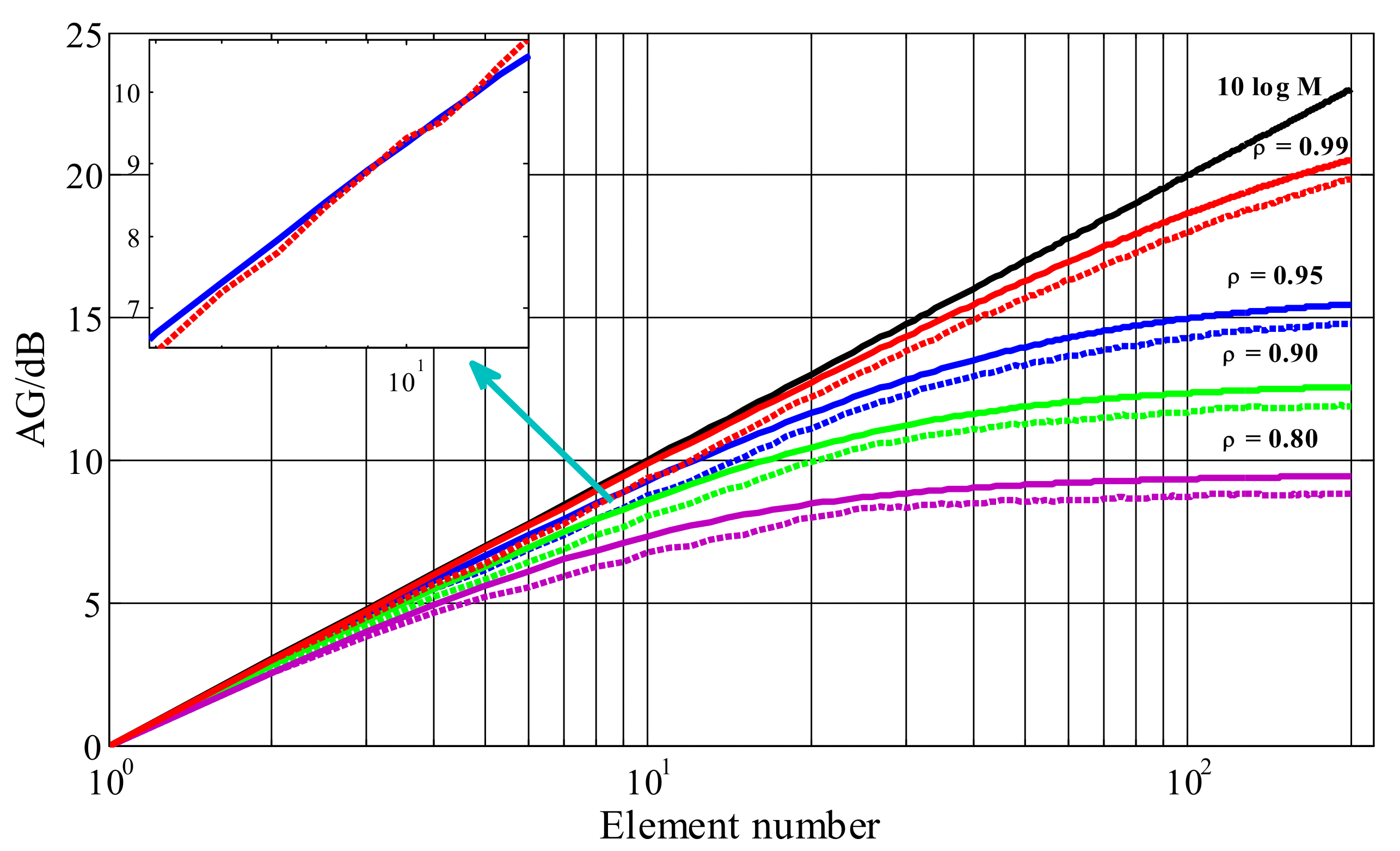
The coherent coefficient is ${\rho }_{ik}={\rho }^{\left|i-k\right|}$ ($\rho$ is the coherence between the acoustic channels at the adjacent elements), which is the same as in ref. [6]. Here, two assumptions are made in the simulation: (1) the $ATL$s’ fluctuation over the elements follows the standard normal distribution; (2) the ambient noise powers are equal and uncorrelated for all pairs of elements. The $A{G}_{\mathrm{U}}$ (colorful solid lines) and $A{G}_{\mathrm{W}}$ (colorful dash lines) as functions of the element number are plotted in Figure 1, where $\rho$ is equal to 0.99, 0.95, 0.90 and 0.80, respectively. For comparison, the ideal value of AG ($10{\log }_{10}M$) is shown by the black solid line. An examination of Figure 1 shows that $A{G}_{\mathrm{U}}$ is always larger than $A{G}_{\mathrm{W}}$ for a given $\rho$. Taking $\rho =0.95$ as an example, the gain of a 200-element array is 15.47 dB for $A{G}_{\mathrm{U}}$, while the corresponding gain for $A{G}_{\mathrm{W}}$ is 14.78 dB for a reduction of 0.69 dB. However, due to the coherence degradation, both $A{G}_{\mathrm{U}}$ and $A{G}_{\mathrm{W}}$ are lower than the ideal value of AG.

It should be noted that the red dash line ($\rho =0.99$ for $A{G}_{\mathrm{W}}$) intersects with the blue solid line ($\rho =0.95$ for $A{G}_{\mathrm{U}}$) when the element number is 10, as shown by the zoomed-in figure in the upper-left corner of Figure 1. Before the intersection point, $A{G}_{\mathrm{U}}$ is larger than or equal to $A{G}_{\mathrm{W}}$, even though the corresponding coherence for $A{G}_{\mathrm{U}}$ is less than that for $A{G}_{\mathrm{W}}$. This illustrates that AG for the weak coherence but without $ATL$’s fluctuation may be smaller than that with strong coherence but large fluctuation of $ATL$. In other words, the propagation loss also affects AG, which should not be ignored in the ocean waveguide.

4.2. Array Gain in the Shallow Water

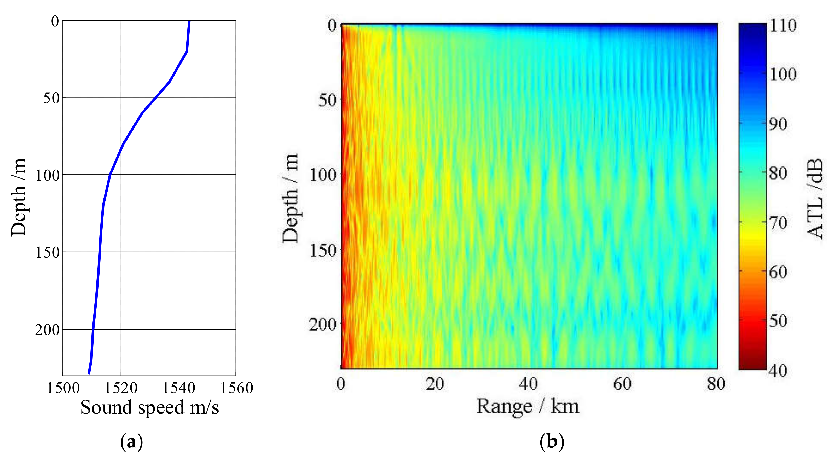
In simulation B, we consider the gain of the HLA in shallow water. The water depth is 229 m with the corresponding SSP as shown in Figure 2a. The source radiating a narrow-band signal with center-frequency 190 Hz is fixed at 110 m. The corresponding $ATL$s are calculated as follows: the transmission loss corresponding to all frequencies within the narrow band is calculated by Kraken program [22] which is developed based on the horizontal-invariant normal model [23]; then $ATL$ can be obtained by Equations (7) and (8). The $ATL$s in shallow water within 80 km is shown in Figure 2b.

The HLA is suspended on a depth of 120 m at the direction of end-fire. We investigate the gain of the HLA at 49 km away from the source, and the corresponding $ATL$s and acoustic channel coherence. The acoustic channel transfer functions corresponding to the HLA are also obtained by Kraken program.

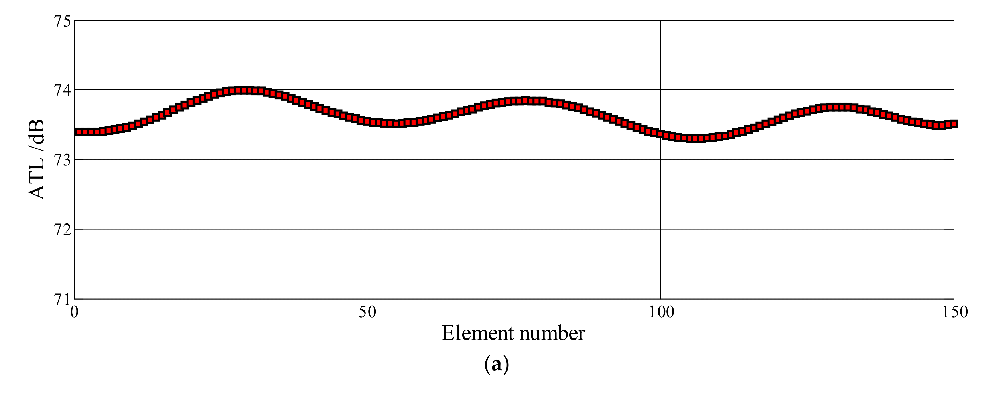
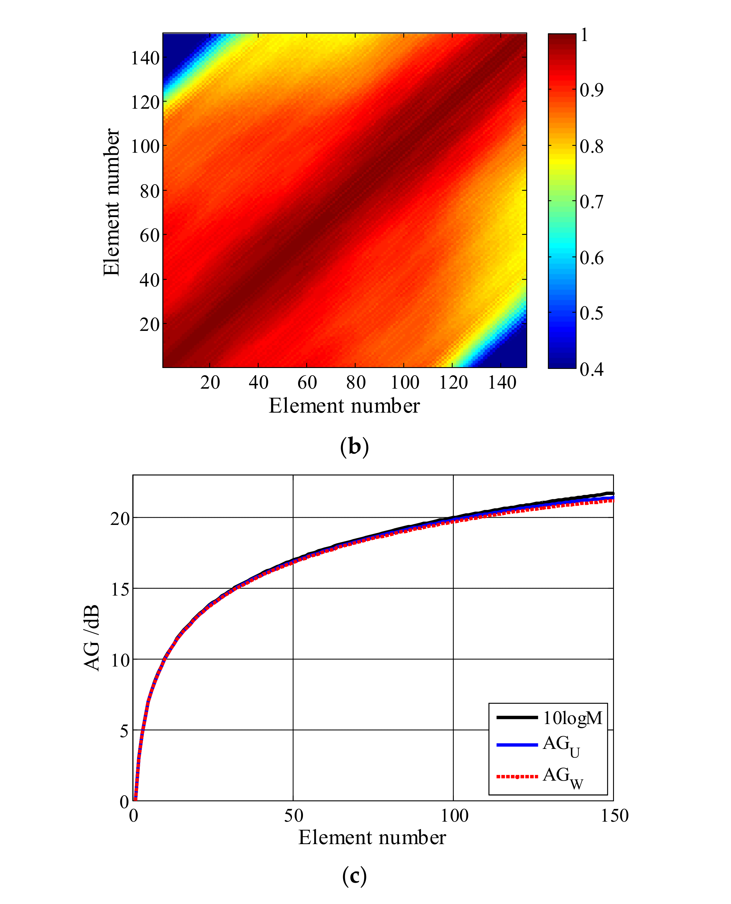
The curve of $ATL$s on the distance 49 km as a function of element number is displayed in Figure 3a. It is observed from Figure 3a that at the 49 km distance, $ATL$s have slight fluctuation with the element number. The variance of $ATL$s’ fluctuation on the HLA is calculated and equal to 0.03 dB. Submitting the acoustic channel transfer functions into Equation (12), we calculate the spatial correlation coefficients between all pairs of the acoustic channels as a function of element number, and the result is shown in Figure 3b. It is observed that at the 49 km distance, the spatial correlation coefficients are almost greater than 0.7, which can be considered as completely coherent [24]. Next, we will investigate the gain of the HLA from transmission loss and acoustic channel coherence.

Firstly, ignoring the fluctuation of $ATL$s (for Case 2), i.e., $\sqrt{p_i}=\sqrt{p_k}$, the expression of array gain can be simplified as Equation (19) that specifies $A{G}_{\mathrm{U}}$. We calculate $A{G}_{\mathrm{U}}$ as the function of element number, and the result is shown by the blue solid line in Figure 3c. Then, using Equation (18) or Equation (20), $A{G}_{\mathrm{W}}$ is also calculated as the function of element number, as shown by the red dash line in Figure 3c. The ideal value of AG ($10{\log }_{10}M$) is shown by the black solid line for comparison. It is observed that both $A{G}_{\mathrm{U}}$ and $A{G}_{\mathrm{W}}$ are close to the ideal value since the acoustic channels are almost completely coherent. In addition, $A{G}_{\mathrm{U}}$ is almost equal to $A{G}_{\mathrm{W}}$, as the result of the slight fluctuation on $ATL$s (in this case, Equation (18) is equivalent to the Equation (19)).

4.3. Array Gain in the Deep Sea

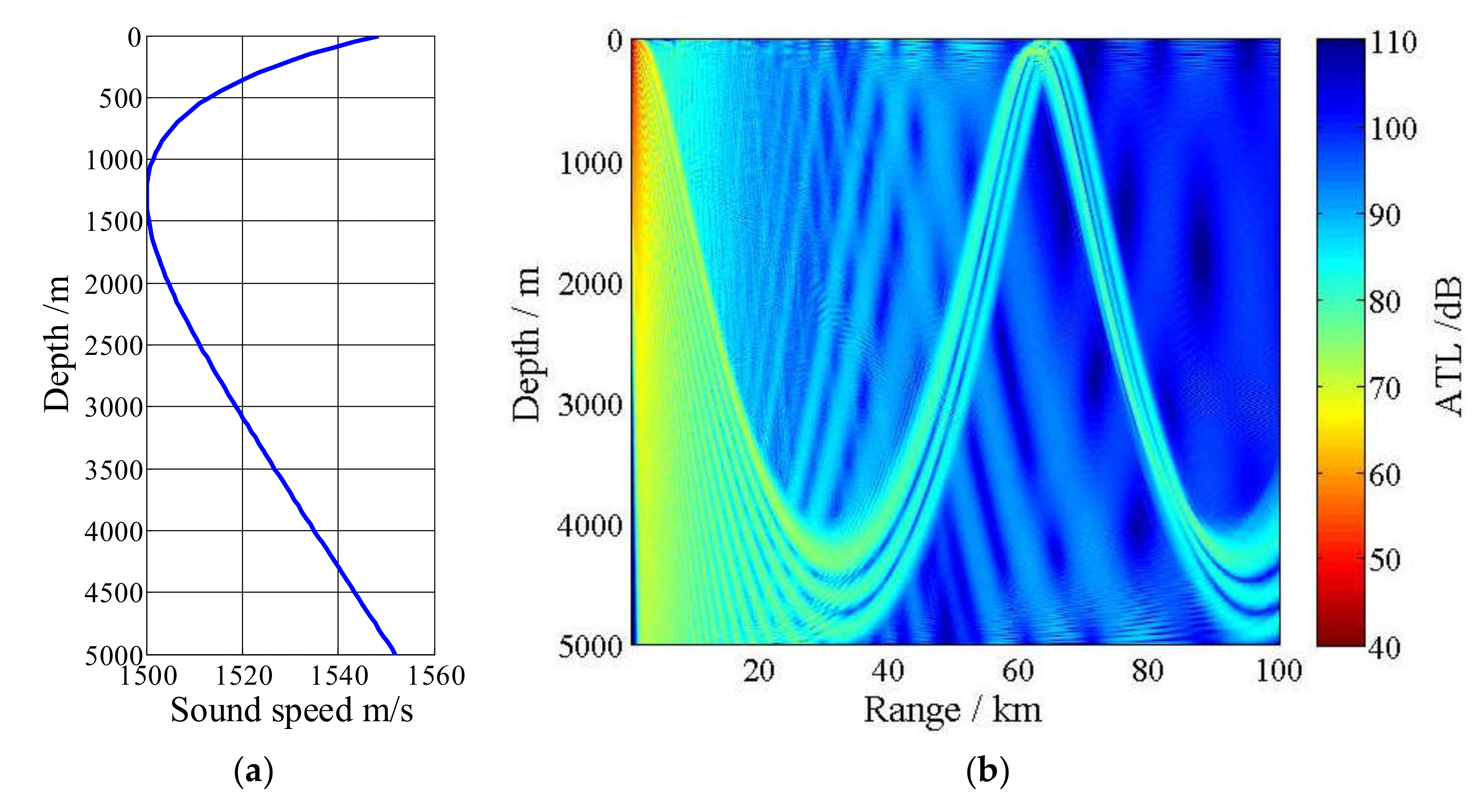
Simulation C considers the gain of the HLA in deep sea with water depth of 5000 m. The SSP of the deep sea is a Munk curve with an acoustic channel axis at 1300 m, as shown in Figure 4a. The source is at a fixed depth of 110 m, radiating a narrow-band signal with a center frequency of 190 Hz (the same as in the simulation B). The $ATL$s can be calculated by Kraken program (the calculation is the same as in simulation B), and the result within 100 km as a function of the sea depth in deep sea is shown in Figure 4b.

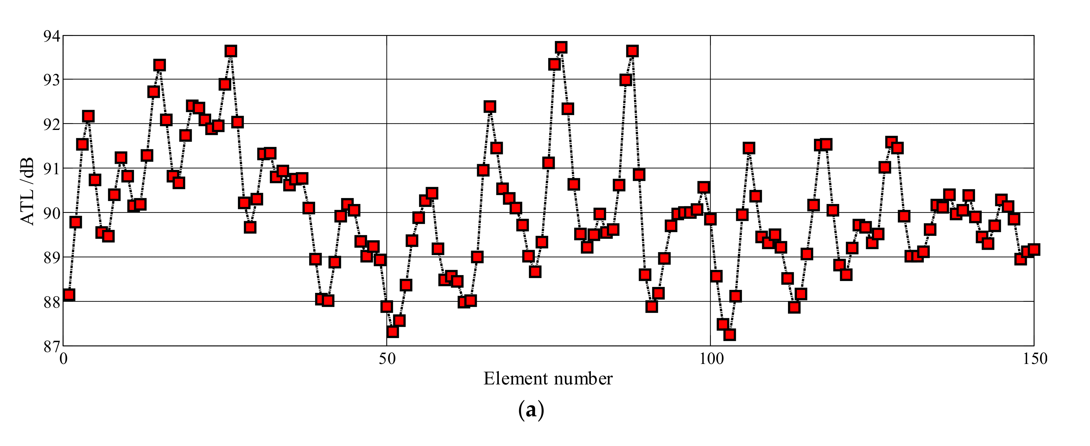
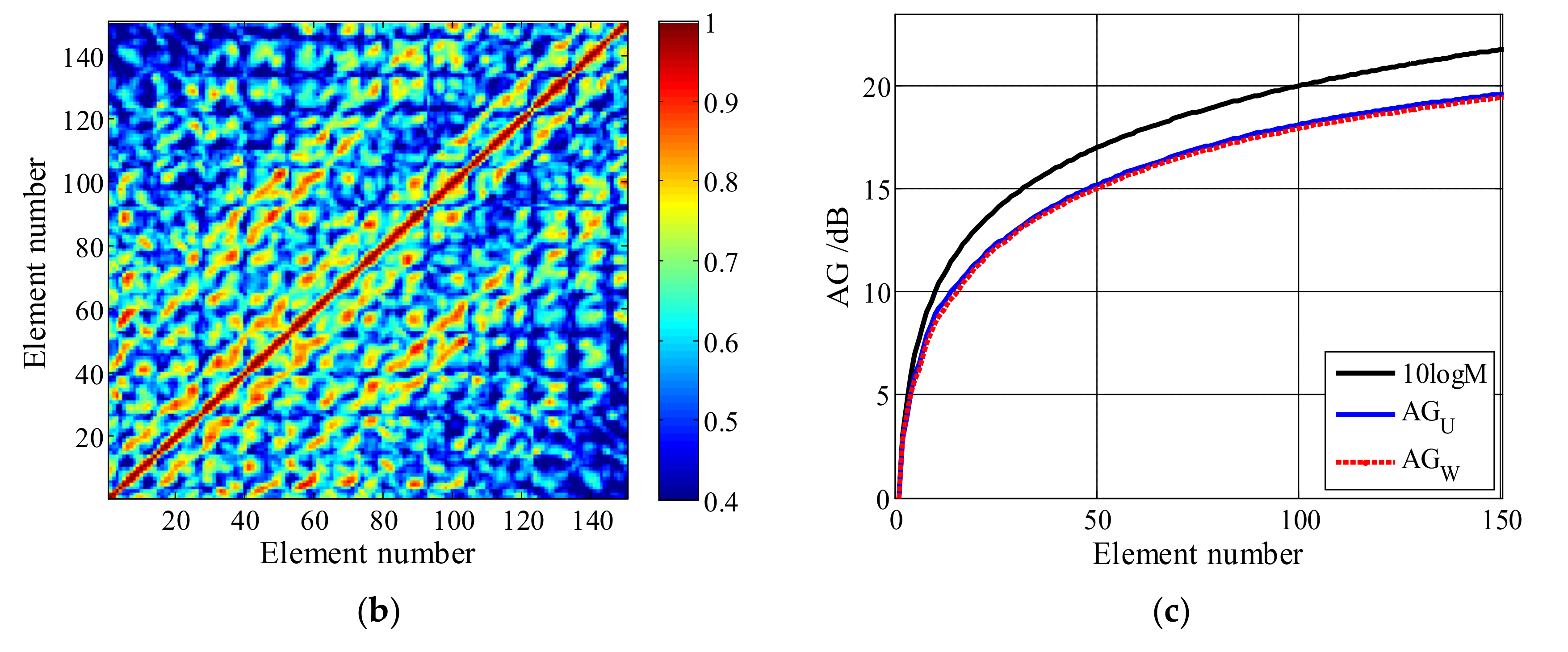
The HLA is at the direction of end-fire, with a receiving depth of 120 m and 20 km away from the source. The sound channel transfer functions corresponding to the HLA are calculated by Kraken program. We calculate $ATL$s at a distance of 20 km as a function of element number, and the result is shown in Figure 5a. It can be observed from Figure 5a that $ATL$s fluctuate with element number greatly, and the fluctuation is greater than that in the simulation B (shallow water). The variance of $ATL$s’ fluctuation on the HLA is calculated and equal to 1.92 dB, which is larger than that in simulation B. Submitting the acoustic channel transfer functions into Equation (12), the spatial correlation coefficients between all pairs of the acoustic channels are calculated as a function of element number, and the result is shown in Figure 5b. Comparing Figure 5b to Figure 3b, it is observed that the correlation coefficients of acoustic channels decrease rapidly as the element spacing increases (the number of elements increases) and is smaller than those in the simulation B. Since AG is affected by $ATL$s and acoustic channel coherence, it can be inferred that the gain will deviate from the ideal value.

Both $A{G}_{\mathrm{U}}$ and $A{G}_{\mathrm{W}}$ corresponding to the HLA are calculated as the function of element number, utilizing Equation (19) and Equation (20), respectively. The results are shown in Figure 5c. It can be observed that both $A{G}_{\mathrm{U}}$ and $A{G}_{\mathrm{W}}$ are less than the ideal value since there is a rapid degradation of acoustic channel coherence. Besides, $A{G}_{\mathrm{W}}$ is smaller than $A{G}_{\mathrm{U}}$ as a result of the fluctuation of $ATL$s, which is different from those in simulation B where $A{G}_{\mathrm{W}}$ is equal to $A{G}_{\mathrm{U}}$.

4.4. Array Gain in the Upslope Waveguide

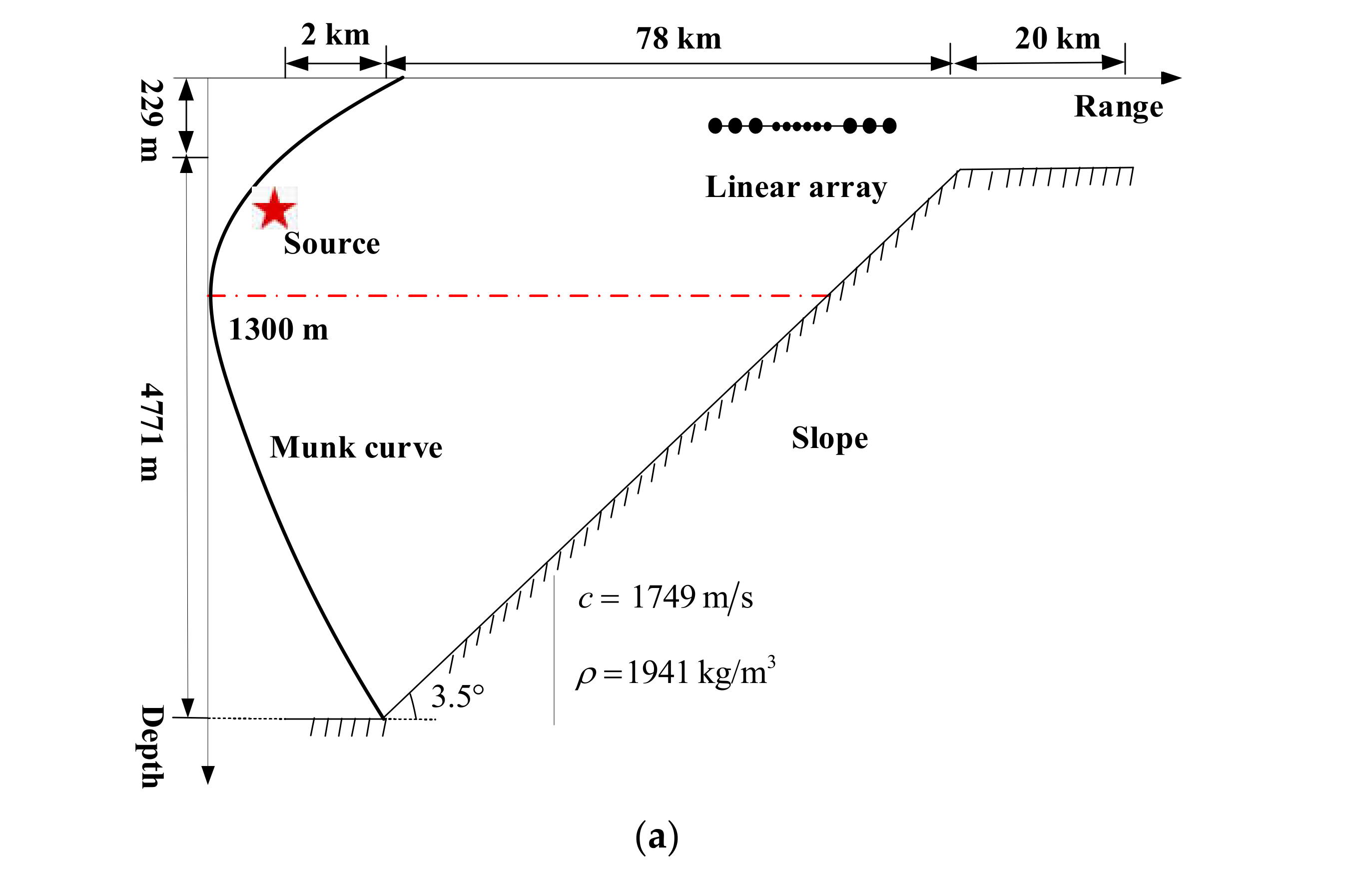
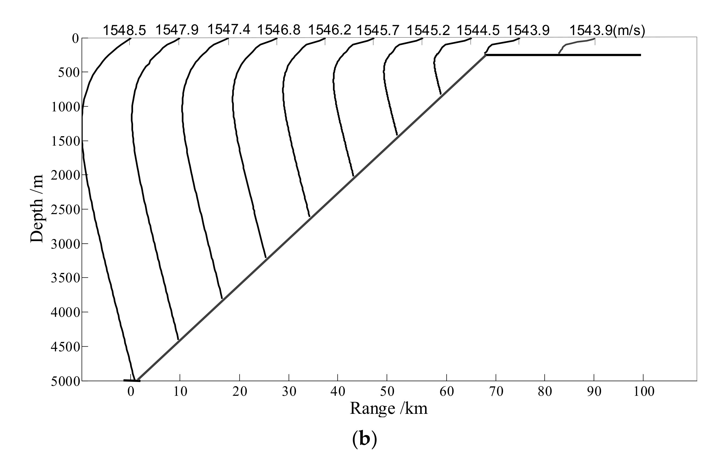
Finally, AG is investigated in the upslope waveguide where the waveguide is range-dependent and the acoustic channels have large fluctuations. The waveguide is shown in Figure 6a, including an abyssal plain (distance of 2 km with water depth of 5000 m), a continental slope (in the 2 to 90 km range, the oblique angle of the bottom is ${3.5}^{\circ }$) and shallow water (distance of 20 km with water depth of 229 m). The SSP of shallow water is a negative gradient, and the SSP of the abyssal sea is the standard Munk curve with a deep sound channel axial at 1300 m. The SSPs of the continental slope region which are range-dependent are shown in Figure 6b.

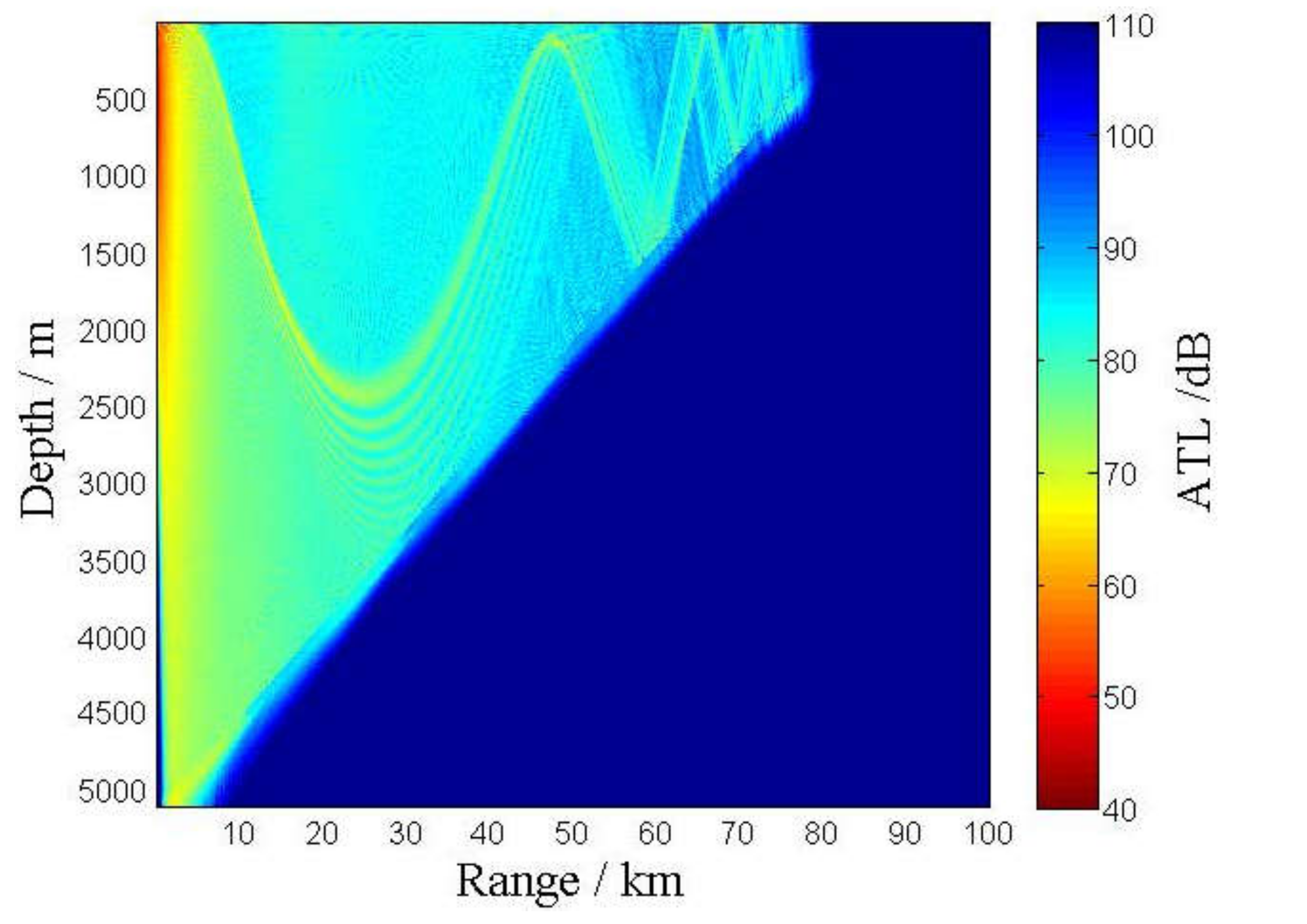
The source is at a fixed depth of 550 m, radiating a narrow-band signal with a center frequency of 190 Hz. The $ATL$s are calculated by RAM program developed on parabolic equations method which is the well-known technique for solving range-dependent propagation problems [25] (the calculation is the same as in simulations B and C). $ATL$s within 100 km in the upslope waveguide are shown in Figure 7.

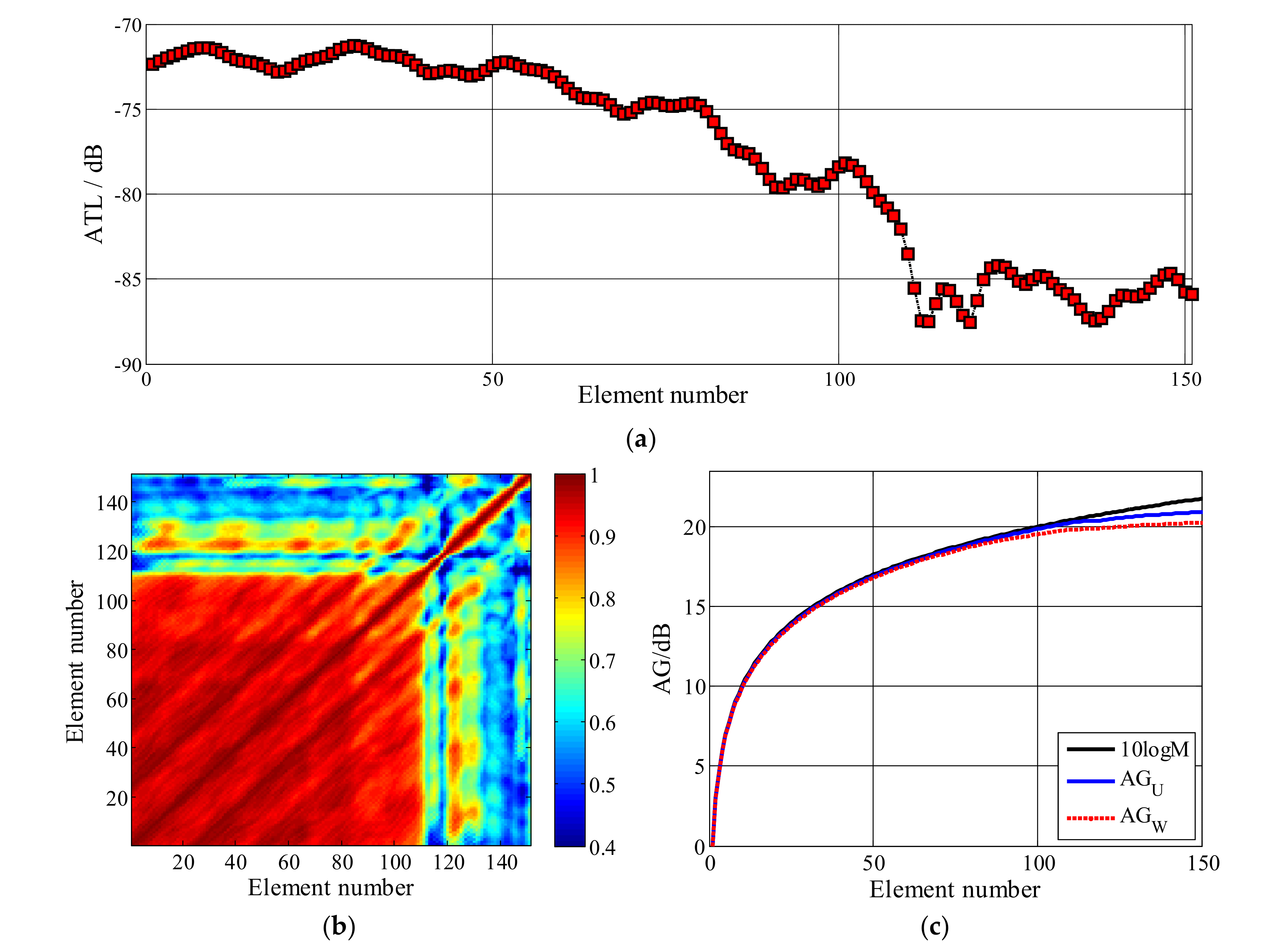
The HLA is suspended at a depth of 120 m, 48 km away from the source (at the direction of end-fire). The $ATL$s at distance 48 km are calculated as the function of element number which are displayed in Figure 8a. As can be seen from the Figure 8a, $ATL$s have rapid fluctuation compared to simulations B (Figure 3a for shallow water) and C (Figure 5a for deep sea). The variance of $ATL$s’ fluctuation is 30.55 dB, which is larger than those in simulations B and C.

The correlation coefficients between two arbitrary acoustic channels corresponding to the elements are shown in Figure 8b. It is observed that when the number of elements is less than 112, the acoustic channels are completely coherent, and the correlation coefficient between any pair of acoustic channels is larger than 0.8. As the number of elements continues to increase (the space between the elements increases), the acoustic channel coherence decreases rapidly.

We investigate $A{G}_{\mathrm{W}}$ and $A{G}_{\mathrm{U}}$ of the HLA in the upslope waveguide. Firstly, for Case 2, ignoring the fluctuation of $ATL$s, $A{G}_{\mathrm{U}}$ is calculated as the function of element number utilized in Equation (19) (equivalent to $A{G}_{\mathrm{U}}$), as shown by the blue solid line in Figure 8c. Then, for Case 3, $A{G}_{\mathrm{W}}$ is calculated by substituting the acoustic transfer functions into Equation (20), and the result is displayed by the red dash line in Figure 8c.

It is observed that $A{G}_{\mathrm{U}}$ are almost equal to the ideal value when the element number is less than 112. Besides, $A{G}_{\mathrm{W}}$ is also close to the ideal value, however, $A{G}_{\mathrm{W}}$ is smaller than $A{G}_{\mathrm{U}}$, due to the fluctuation of $ATL$s on the elements (the variance of $ATL$s’ fluctuation on 112 elements is 11.6 dB).

When the number of elements is more than 112, as the acoustic channel coherence degradation, both $A{G}_{\mathrm{W}}$ and $A{G}_{\mathrm{U}}$ are lower than the ideal value. In addition, it is observed that $A{G}_{\mathrm{W}}$ is less than $A{G}_{\mathrm{U}}$, and the deviation of $A{G}_{\mathrm{W}}$ from the ideal value is more severe. This is because the $ATL$s fluctuate more severely when the number of elements keep increasing (more than 112), as shown in Figure 8a.

From the above simulations, it can be inferred that AG is determined by both transmission loss and acoustic channel coherence. For the completely coherent acoustic channels, AG is almost equal to the ideal value. The result of traditional method for AG in ocean waveguide is too large. The reason is that the effect of the transmission loss fluctuation with elements on AG is ignored in the traditional method. The numerical results verify the theory in Section 3.

5. Conclusions

The degradation of AG in the ocean waveguide is investigated in the paper from the fluctuant acoustic channels that can be depicted with the fluctuant propagation loss and the acoustic channel coherence degradation. A general formula of AG for a linear array in the ocean waveguide is derived as Equation (18) under the assumption that the ambient noise is isotropic. The formula takes full account of the influence of acoustic channels and can be applied to shallow water, deep sea, and continental slope area. Furthermore, we prove that the traditional formula of AG (by Urick) is only a special case of the formula presented in this paper. An analysis of AG for a uniform linear array is presented that provides some insight into the physics of the problem of the array performance in the ocean waveguide. We have found that the obtained AG in the ocean waveguide is reduced compared to that calculated by the traditional method. The numerical simulations compare AGs obtained by the traditional method and the proposed method in four scenarios, including the acoustic channel coherence decreasing exponentially, shallow water, deep sea, and upslope waveguide. Numerical results show that (1) the stronger the acoustic channel coherence, the greater AG; (2) $A{G}_{\mathrm{U}}$ is almost equal to$A{G}_{\mathrm{W}}$ when the fluctuation of $ATL$s is small; (3) $A{G}_{\mathrm{U}}$ will be always be larger than $A{G}_{\mathrm{W}}$ if the fluctuation of the propagation losses is ignored. It is inferred that both acoustic channel coherence and transmission loss fluctuation should be considered when calculating AG in ocean waveguide.

References

- Urick, R.J. Principles of Underwater Sound for Engineers; McGraw-Hill: New York, NY, USA, 1967; p. 33. ISBN 9780070660854. [Google Scholar]
- Van Trees, H.L. Optimum Array Processing: Part IV of Detection, Estimation, and Modulation Theory; John Wiley and Sons Inc.: New York, NY, USA, 2002; pp. 63–66. ISBN 978-0471093909. [Google Scholar]
- Uscinski, B.J.; Reeve, D.E. The effect of ocean inhomogeneities on array output. J. Acoust. Soc. Am. 1990, 87, 2527–2534. [Google Scholar] [CrossRef]
- Neubert, J.A. Effect of the sound field structure on array signal gain in a multipath environment. J. Acoust. Soc. Am. 1981, 70, 1098–1102. [Google Scholar] [CrossRef]
- Carey, W.M.; Reese, J.W.; Stuart, C.E. Mid-frequency measurements of array signal and noise characteristics. IEEE J. Ocean. Eng. 1997, 22, 548–565. [Google Scholar] [CrossRef]
- Gao, S.W.; Griffiths, J.W.R. Experimental performance of high-resolution array processing algorithms in a towed sonar array environment. J. Acoust. Soc. Am. 1994, 95, 2068–2080. [Google Scholar] [CrossRef]
- Stergiopoulos, S. Limitations on towed-array gain imposed by a nonisotropic ocean. J. Acoust. Soc. Am. 1991, 90, 3161–3172. [Google Scholar] [CrossRef]
- Brown, J.L. Variation of array performance with respect to statistical phase fluctuations. J. Acoust. Soc. Am. 1962, 34, 1927–1928. [Google Scholar] [CrossRef]
- Berman, H.G.; Berman, A. Effect of correlated phase fluctuation on array performance. J. Acoust. Soc. Am. 1962, 34, 555–562. [Google Scholar] [CrossRef]
- Lord, G.E.; Murphy, S.R. Reception characteristics of a linear array in a random transmission medium. J. Acoust. Soc. Am. 1964, 36, 850–854. [Google Scholar] [CrossRef]
- Heaney, K.D. Shallow water narrowband coherence measurements in the Florida Strait. J. Acoust. Soc. Am. 2011, 54, 2026–2041. [Google Scholar] [CrossRef] [PubMed]
- Wan, L.; Badiey, M. Horizontal coherence of sound propagation in the presence of internal waves on the New Jersey continental shelf. J. Acoust. Soc. Am. 2015, 137, 2390. [Google Scholar] [CrossRef]
- Cox, H. Line array performance when the signal coherence is spatially dependent. J. Acoust. Soc. Am. 1973, 54, 1743–1746. [Google Scholar] [CrossRef]
- Green, M.C. Gain of a linear array for spatially dependent signal coherence. J. Acoust. Soc. Am. 1976, 60, 129–132. [Google Scholar] [CrossRef]
- Carey, W.M. The determination of signal coherence length based on signal coherence and gain measurements in deep and shallow water. In Proceedings of the Oceans’ 97 MTS/IEEE Conference, Halifax, NS, Canada, 6–9 October 1997; pp. 462–470. [Google Scholar] [CrossRef]
- Carey, W.M.; Moseley, W.B. Space-time processing, environmental-acoustic effects. IEEE J. Ocean. Eng. 1991, 3, 285–301. [Google Scholar] [CrossRef]
- Carey, W.M. Sonar array characterization, experimental results. IEEE J. Ocean. Eng. 1998, 23, 297–306. [Google Scholar] [CrossRef]
- Hamson, R.M. The theoretical gain limitations of a passive vertical line array in shallow water. J. Acoust. Soc. Am. 1980, 68, 156–164. [Google Scholar] [CrossRef]
- Buckingham, M.J. Array gain of a broadside vertical line array in shallow water. J. Acoust. Soc. Am. 1979, 65, 148–161. [Google Scholar] [CrossRef]
- Gaul, R.D.; Knobles, D.P.; Shooter, J.A.; Wittenborn, A.F. Ambient noise analysis of deep-ocean measurements in the Northeast Pacific. IEEE J. Ocean. Eng. 2007, 32, 497–512. [Google Scholar] [CrossRef]
- Xie, L.; Sun, C.; Jiang, G.Y.; Liu, X.H.; Kong, D.Z. Effect of the fluctuant acoustic channel on the gain of a linear array in the ocean waveguide. Chin. Phys. B 2018, 27, 114301. [Google Scholar] [CrossRef]
- Porter, M.B. The KRAKEN Normal Mode Program; Naval Research Lab: Washington, DC, USA, 1992. [Google Scholar]
- Jensen, F.B.; Kuperman, W.A.; Porter, M.B.; Schmidt, H. Computational Ocean Acoustics; Springer Science & Business Media: New York, NY, USA, 2011; pp. 337–402. [Google Scholar] [CrossRef] [Green Version]
- Wille, P.; Thiele, R. Transverse horizontal coherence of explosive signals in shallow water. J. Acoust. Soc. Am. 1971, 50, 348–353. [Google Scholar] [CrossRef]
- Collins, M.D. Generalization of the split-step pade solution. J. Acoust. Soc. Am. 1994, 96, 382–385. [Google Scholar] [CrossRef]
Figure 1.
(colorful solid line) and (dash line) as a function of the number of elements for different , with the black solid line showing the ideal value of AG.
Figure 2.
Simulation parameters and sound propagation in shallow water: (a) The sound speed profile; (b) The average transmission loss.
Figure 3.
Fluctuant acoustic channels and AGs for the receiving depth of 120 m and distance of 49 km in the shallow water: (a) s on the elements; (b) Correlation coefficients; (c) (blue solid line), (red dash line) and the ideal value of AG (black solid line) varying with the element number.
Figure 4.
Simulation parameters and sound propagation in deep sea: (a) The sound speed profile; (b) The average transmission loss.
Figure 5.
Fluctuant acoustic channels and AGs for the receiving depth of 120 m and distance of 20 km in the deep sea: (a) s on the elements; (b) Correlation coefficients; (c) (blue solid line), (red dash line) and the ideal value of AG (black solid line) varying with the element number.
Figure 6.
The upslope waveguide: (a) Simulation environment and parameters; (b) The SSPs of the continental slope region.
Figure 7.
Average transmission loss in the upslope waveguide when the source depth is 550 m.
Figure 8.
Fluctuant acoustic channels and AGs for the receiving depth of 120 m and distance of 48 km in the upslope waveguide: (a) on the elements; (b) Correlation coefficients; (c) (blue solid line), (red dash line) and the ideal value of AG (black solid line) varying with the element number.
Publisher’s Note: MDPI stays neutral with regard to jurisdictional claims in published maps and institutional affiliations. |
© 2021 by the authors. Licensee MDPI, Basel, Switzerland. This article is an open access article distributed under the terms and conditions of the Creative Commons Attribution (CC BY) license (https://creativecommons.org/licenses/by/4.0/).
Share and Cite
MDPI and ACS Style
Liu, Z.-W.; Yang, C.-M.; Jiang, Y.; Xie, L.; Du, J.-Y.; Lü, L.-G. Array Gain of a Linear Array in an Ocean Waveguide. Appl. Sci. 2021, 11, 5046. https://0-doi-org.brum.beds.ac.uk/10.3390/app11115046
AMA Style
Liu Z-W, Yang C-M, Jiang Y, Xie L, Du J-Y, Lü L-G. Array Gain of a Linear Array in an Ocean Waveguide. Applied Sciences. 2021; 11(11):5046. https://0-doi-org.brum.beds.ac.uk/10.3390/app11115046
Chicago/Turabian StyleLiu, Zong-Wei, Chun-Mei Yang, Ying Jiang, Lei Xie, Jin-Yan Du, and Lian-Gang Lü. 2021. "Array Gain of a Linear Array in an Ocean Waveguide" Applied Sciences 11, no. 11: 5046. https://0-doi-org.brum.beds.ac.uk/10.3390/app11115046
Note that from the first issue of 2016, this journal uses article numbers instead of page numbers. See further details here.