
Edge-Preserving Image Denoising Based on Lipschitz Estimation


1
Istituto di Scienza e Tecnologie dell’Informazione “Alessandro Faedo” CNR, 56124 Pisa, Italy
2
Department of Cyber Security, Air University, Islamabad 44000, Pakistan
3
Le2i, VIBOT ERL CNRS 6000, Universite de Dijon, 71200 Dijon, France
*
Author to whom correspondence should be addressed.
Appl. Sci. 2021, 11(11), 5126; https://0-doi-org.brum.beds.ac.uk/10.3390/app11115126
Submission received: 27 April 2021
/
Revised: 19 May 2021
/
Accepted: 28 May 2021
/
Published: 31 May 2021
(This article belongs to the Special Issue Advances in Signal, Image and Video Processing)
Abstract
:The information transmitted in the form of signals or images is often corrupted with noise. These noise elements can occur due to the relative motion, noisy channels, error in measurements, and environmental conditions (rain, fog, change in illumination, etc.) and result in the degradation of images acquired by a camera. In this paper, we address these issues, focusing mainly on the edges that correspond to the abrupt changes in the signal or images. Preserving these important structures, such as edges or transitions and textures, has significant theoretical importance. These image structures are important, more specifically, for visual perception. The most significant information about the structure of the image or type of the signal is often hidden inside these transitions. Therefore it is necessary to preserve them. This paper introduces a method to reduce noise and to preserve edges while performing Non-Destructive Testing (NDT). The method computes Lipschitz exponents of transitions to identify the level of discontinuity. Continuous wavelet transform-based multi-scale analysis highlights the modulus maxima of the respective transitions. Lipschitz values estimated from these maxima are used as a measure to preserve edges in the presence of noise. Experimental results show that the noisy data sample and smoothness-based heuristic approach in the spatial domain restored noise-free images while preserving edges.
1. Introduction
Several industrial imaging systems are widely employed in different applications of Non-Destructive Testing (NDT). The presence of noise elements or degradation added during the testing process can directly affect the performance of the evaluation. In general, denoising such data (in the form of a signal or image) involves removing these degradations while capturing and transmitting signals or images. These degradations are commonly categorized as blur or noise. Blurring, the most common type of degradation, involves bandwidth reduction due to a problem in the image formation. There can be several reasons for this imperfection. Most commonly, these problems occur due to the relative motion of the camera and the original scene or due to an out of focus optical system.
In addition to these blurring effects, the recorded image is corrupted by additional noise elements. These additional noise elements are introduced during the transmission via a noisy channel or errors during the measurement process and directly affect the performance of NDT. Therefore, it is of extreme importance to reduce noise and preserve the sharpness of edges without introducing blurring. Goyal et al. evaluated the most state-of-the-art image denoising methods in [1].
Methods proposed in the past are mainly categorized into spatial domain and transform-based techniques. The selection is dependent on the application and the nature of noise present in the image. Denoising in the spatial domain is performed using linear methods based on an averaging filter, e.g., Gabor proposed a model based on Gaussian smoothing [2], and edge detection-based denoising using anisotropic filtering [3,4,5]. Yaroslavsky and Manduchi used a neighborhood filtering method [6,7]. Image denoising in the spatial domain is complex and more time-consuming especially for real-time problems.
Some researchers worked in the frequency domain to denoise images, e.g., Wiener filters [6]. Chatterjee and Milanfar improved the performance of denoising by taking advantage of patch redundancy from the Weiner filter-based method [8]. The scope of these linear techniques is limited to stationary data, as the Fourier transform is not suitable to perform analysis on non-stationary and nonlinear data. As a result, denoising methods based on multi-scale denoising employing nonlinear operations in the transform domain came up as an alternative. These multiple scales provide sparse representation of the signal in the transform domain.
Several methods based on wavelet transform have been proposed in the past [9,10,11,12,13,14,15]. A brief survey of some of these methods is given by Buades et al. in [16,17]. Seo et al. presented a comparison and discussion on the kernel based methods [18]. The method proposed by Blu and Luisier minimized the mean square error estimate termed as —Stein’s unbiased risk estimate (SURE) [19]. In another method, dual tree complex wavelets were transformed into ridgelet transforms by Chen and Kegl [20]. Starck et al. proposed image denoising based on the family of transforms—the ridgelet and curvelet transforms—as alternatives to the wavelet representation of image data [12].
Similarly, Tessens et al. used curvelet coefficients to distinguish two classes of coefficients, e.g., noise-free components, which they termed as “signal of interest,” and other [10]. More recently, Pesquet et al. adopted a hybrid approach that combined frequency and multi-scale analysis [13]. They formulated the restoration problem as a nonlinear estimation problem leading to the minimization of a criterion derived from Stein’s unbiased quadratic risk estimate. Alkinani et al. investigated patch-based denoising methods for additive noise reduction [21]. Recently, Naveed et al. proposed DWT- and DT-CWT-based image denoising methods and employed statistical goodness of fit tests on wavelet coefficients at multi-scales to identify noise at different levels [22].
Bnou proposed a method based on an unsupervised learning model. They presented adaptive dictionary learning-based denoising of approximation. The wavelet coefficients were denoised by using an adaptive dictionary learned over the set of extracted patches from the wavelet representation of the corrupted image [23]. Several other methods have also been proposed in the past, but there is limited study regarding the preservation of edges.
Recently, Paras and Vipin presented a brief evolution of the research on edge-preserving denoising methods in [24], and Pizurica presented an overview of image denoising algorithms ranging from wavelet shrinkage to patch-based non-local processing with the main focus on the suppression of additive Gaussian noise [25]. Pal et al. reviewed the benchmark edge-preserving smoothing algorithms and keeping the main focus on anisotropic diffusion and bilateral filtering [26].
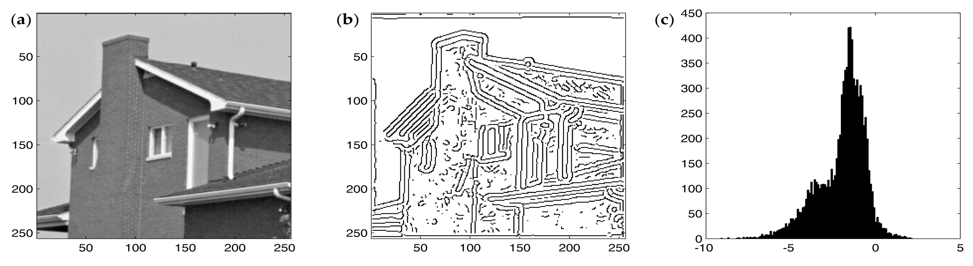
Many other filtering algorithms exists but, as mentioned before, very few of them discussed the edges and the spurious oscillations or artifacts introduced after denoising. Gibbs phenomena explain these oscillations in the neighborhood of discontinuities. An edge separates two different areas with limited or no connections between them e.g., no common characteristics: texture, noise, etc. Figure 1a, presents an edge part of the House image.
Figure 1b,c represents the same image with the addition of white Gaussian noise and denoised image [19]. It can be observed from the figure that, while denoising, some additional artifacts have been produced. This is because most linear or nonlinear methods use neighborhood pixels while denoising. It is, therefore, logical to separate edges and transitions from the rest of the background.
Most of the wavelet-based methods use Discrete Wavelet Transform (DWT) for denoising; however, DWT suffers from three main issues, lack of shift-invariant, poor directional, and lack of phase information. Stationary wavelet transform reduced the problem of partial translation in variance and considerably improved the denoising results; however, it suffers from the cost of very high redundancy and is ultimately computationally expensive. Many algorithms have been proposed to solve the shortcomings of DWT by using different forms of Complex Wavelet Transforms (CWT) [27].
CWT is nearly translation invariant with directional selectivity but at the cost of high redundancy, [27]. Similarly, through continuous wavelet transform analysis, a set of wavelet coefficients is obtained, indicating how close the signal is to a particular basis function. Since the continuous wavelet transform behaves like orthonormal basis decomposition, it can be shown that it is isometric, i.e., it preserves energy [28]. Hence, the signal can be recovered from its transform.
The wavelet transform in its continuous form can accurately represent minor variations/edges present in signal. In most of the denoising methods, these minor variations that correspond to the edges of different levels in images are not considered while denoising. In this work, we classify this separation as classes for edges and background using continuous wavelet transform. This classification is based on the information obtained from the Lipschitz estimation.
The rest of the paper is organized as follows. Section 2 introduces the method and the principle of method. Section 3 gives a detailed explanation of the multi-scale analysis based edge detection. In Section 4, we present the Lipschitz regularity in the context of images, followed by the explanation of the reconstruction method. Section 5 explains the obtained results and evaluates the performance of the proposed method, and Section 6 finally concludes the paper.
2. Method
We identified transitions and restored noise-free image using heuristic approach. Initially, all significant edges where the intensity changes abruptly were identified by using the modulus maxima approach using multiscale analysis. Based on the detection of edges from modulus maximas, we classified the information from the image into the edge and background. Lipschitz exponents based reconstruction resulted in noise-free images. The edges where the intensity changes abruptly preserved their Lipschitz estimation even with the addition of noise.
Principle of the Method
We assume that the image is corrupted by different types of noise. In this work, we focused on white Gaussian noise with a zero mean. The given image is specified in the model:
f is the noise-free signal, uniformly sampled (e.g., an image) and is the white Gaussian noise with 0 mean and variance. In the present work, the given data will always be an matrix with . The aim is to estimate the function with respect to an estimator such that:
In order to estimate the function F, the method is proposed to preserve the energy of the strong edges by separating them from the background. The restoration based on data samples and smoothing results in noise-free images. The block diagram of the method is given in Figure 2.
3. Multi Scale Analysis Based Edge Detection
Edges correspond to the intensity changes in an image and separate two different regions by defining their boundary. In most denoising methods, while suppressing noise elements and the smoothing process, significant changes are introduced in the high-frequency elements which correspond to the edges. The main purpose of this paper is to preserve the sharpness of these high-intensity elements and, to do so, we employed wavelet transform-based multi-scale analysis. We decomposed the image into different scales and detected the local minima and maxima at each level. The multi scale was performed by smoothing the surface with the convolution kernel that is dilated, correspond to the Gaussian function [27]. The wavelet transform components are proportional to the coordinates of the gradient vector of f smoothed by :
If corresponds to the intensity image after wavelet transformation, then the discrete version can be written as [27]:
and correspond to the gradients in the horizontal and vertical directions, respectively. The gradient image in both directions (horizontal and vertical) of the House image is given in Figure 3a,b respectively.
Local Maxima Extraction
The maxima across each scale were extracted from the gradient of the image and by following the direction of the phase angle. The comparison of gradients from the neighborhood pixels classified the current pixel as the local maxima or otherwise. The current pixel can only be the local maxima if it satisfies the following condition:
where represents the gradient in the positive phase angle of the neighborhood pixel, represents the gradient in the negative phase angle of the neighborhood pixel, and corresponds to the gradient of the current pixel/point. Figure 4b illustrates the detected maxima of the image representing the edges of the House, the background, and noise. We employed Median Absolute Deviation (MAD)-based thresholding to eliminate noise and background maxima from the main structure of the image. Figure 4 illustrates the corresponding maxima before and after applying thresholding.
In signal feature extraction, the selection of the mother wavelet function is directly affected by the characteristics of the signal/image. In this context, to extract the most useful information, the selection of wavelet function is of extreme importance. At the same time, while computing the modulus maxima, it is not guaranteed that the modulus maxima is located at a point belonging to a maxima line that propagates toward a finer line. Mallat highlighted that, when the scale decreases, may have no more maxima in the neighborhood of . He proved that by using the diffusion equation that this would never be the case if the wavelet function is a derivative of Gaussian. Hence, the derivative of a Gaussian function has an important property of continuous differentiability, which makes this function suitable for the analysis of most type of signals [27].
4. Lipschitz Based Image Restoration
In order to perform the restoration process, we computed Lipschitz exponents to identify strong edges. These exponents were estimated using modulus maxima lines. The modulus maxima curves are defined as the lines along which all points correspond to the modulus maxima. In the case of images, these maxima lines can be traced by following the neighborhood of local maxima in successive scales as shown in Figure 5. The boundary of some important structures can be traced by following the series of maxima that are normally distributed along the edge curve.
Wavelet maxima that correspond to the common edge at different scales are chained together by following the direction of the tangent to create the maxima curve of the respective edge at different scale levels. Therefore, by comparing the phase of edge points with the phase of an adjacent neighborhood in the next scale, it can give the pixel that corresponds to the maxima curve. It was shown by Mallat that point-wise singularities can be computed by measuring the decay of the slope of the logarithmic function of the coefficient of magnitude along the logarithmic function of scales, and this is termed as the Lipschitz exponent.
4.1. Lipschitz Regularity in the Context of Images
The Lipschitz regularity of a two dimensional function (image) f is related to the asymptotic decay of and in the corresponding neighborhood, and this decay is dependent on the magnitude defined by . It was proven by Mallat that f is uniformly Lipschitz inside the bounded domain of , if and only if there exist a constant A > 0 such that for all the u inside this domain and all scales [27]:
However, we are concerned with the pointwise regularity in 2D. Therefore, by using the local maxima lines, we have computed the Lipschitz regularity by using Equation (9). In Figure 6 and Figure 7 from the histogram of the Lipschitz estimation, it is estimated that, in the present case, the Lipschitz value lies in a certain range.
4.2. Restoration
In order to obtain a noise-free image from the background, the method utilizes data samples and performs non linear functioning to estimate the best fit. We defined an adaptive restoration method for two classes: one for the edges and one for the background. The concept of the class definition is given in Figure 8a. The edge points belong to class 1 and rest of the image belong to class 2. While denoising, we centered the pixel on a window.
The weighting factor depends on the adjacent neighborhood of the respective class. The method restores each pixel by taking into account extracted edge and background pixel based on their respective Lipschitz exponents. The method preserve edges and restores the background by utilizing noisy samples and their smoothness to estimate the best fit. Initially, we defined the deterministic function in terms of the smoothness and mean square error estimation as:
where corresponds to the size of the image and k defines the iteration step. is the mean square error estimation of the restored subset with the original signal of respective subset such that
defines the smoothness of the reconstructed subset signal. In this context, each pixel will generate the equation according to the adjacent neighborhood (as explained in Figure 8) for smoothing:
where for each pixel depends on if the current pixel corresponds to the background or an edge, and hence, based on that, the assigned value would be “1” or it would correspond to “0” as illustrated in Figure 8b.
In order to simplify Equation (10), we consider the Taylor series expansion to find the value of and and for the given series, the minimum mean square error correspond to , therefore, by simplifying the Taylor series expansion:
and we know that:
As and , the variables in Equation (15) can be replaced such that
Thus,
and we can simplify the equation to
Similarly by using the Taylor series on the smoothing criteria, is as follows:
In order to determine the best estimation of the deterministic function and minimum error between the restored pixel and the original pixel of either background or an edge, the algorithm works in the iterative mode. We assume the least smoothness of the respective pixels for initialization. Two optimization factors, for noisy samples and for smoothness, are introduced (in Equation (10) to investigate the most optimal compromise between the data samples containing noise and their smoothness such that Equation (10) will become:
Parametric Estimation
In order to estimate and , we can write Equation (20) in the discrete case by simplifying as,
where correspond to the adjacent neighbors, The value of is dependent on whether the current pixel belongs to the edge or background but, in any case, should satisfy the stability conditions. The term that corresponds to the mean square error in Equation (20) is stable due to the presence of the original noisy pixel, and hence these factors were computed in terms of the smoothness criteria, and Equation (21) can be rewritten as:
The Equation (22), should satisfy the following condition in order to ensure the stability of the signal:
The stable range to define the constant term in numerical form between to is obtained by considering the above conditions. Hence, based on these findings, we define two constant factors in term of an equation:
All pixels were restored individually taking into account the neighbor pixels of the same class. The complete algorithm is given in the Appendix A.
5. Results and Analysis
This section presents the performance evaluation of the proposed algorithm. The set of set of images used for experimentation consisted of standard test images, including House, Lena, Circuit, Pepper, and Hand, and were tested with various noise levels. The images were corrupted with the addition of Gaussian noise of zero mean and standard deviation ranging from 15 to 35.
The peak signal to noise ratio (PSNR) was employed as the measure of quantitative performance as explained in Section 2. We computed Lipschitz exponents to identify the edges or image structure. These exponents were estimated using the modulus maxima lines. We analyzed these estimations with the addition of Gaussian white noise (28 dB). In order to illustrate more detailed analysis, we show in Figure 9, a single row (125) of the image as a curve without and with the addition of noise. It can be seen from the results that sharp transitions preserved their Lipschitz estimation even in the presence of noise.
To illustrate the robustness of the estimation () in the case of natural images, we analyzed our test samples in the case of a constant affine transformation, as shown in Figure 10. The original image has been deformed by the 10 of rotation. Lipschitz exponents were estimated, and, from the histogram, we observed that approximately 92% of the Lipschitz regularity values lay in between the same range. The regularity () was preserved even when a constant affine deformation was applied to an image.
Therefore, we concluded from our findings that the Lipschitz exponents can be used as a significant measure to study natural images. At the same time, the problem of preserving edges in any linear or nonlinear denoising algorithm can be handled with this estimation. The transitions identified based on their Lipschitz exponents represent the main structure of the image; therefore, we preserved these points and performed smoothing on the rest of the image, as explained in the Section 4.
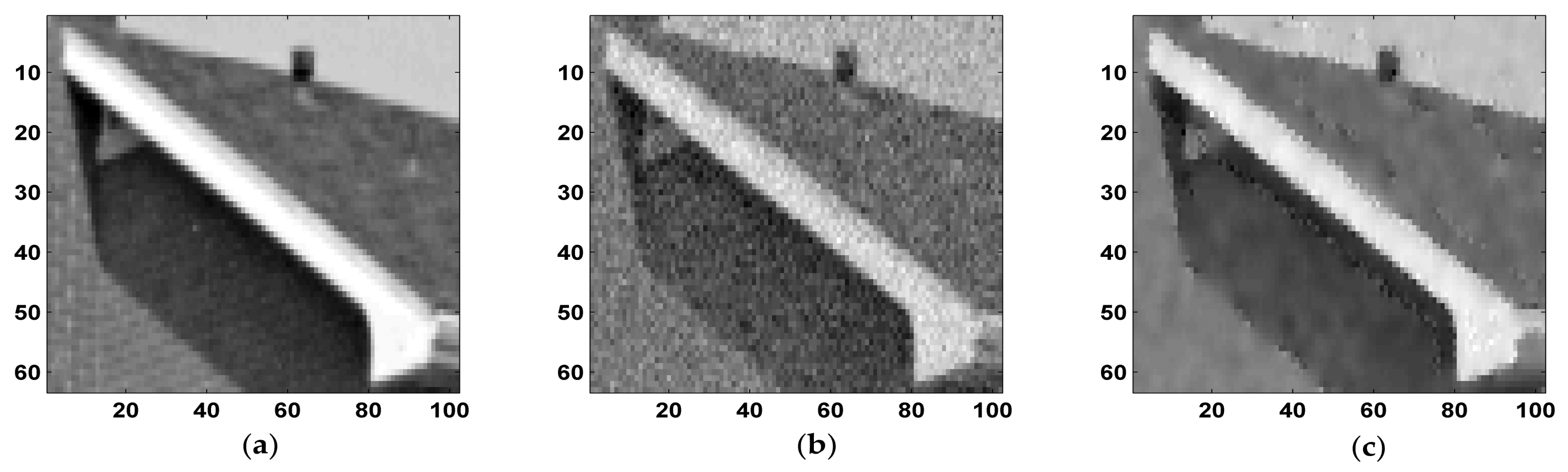
We defined an adaptive restoration method and performed data samples based nonlinear functioning to estimate the best fit. The method restores therest of the image by utilizing noisy sample and their smoothness. As an example, Figure 11 illustrates the focused edges of the image overlaid with the results of edge extraction. Noise level of 24.59 dB PSNR were added and by performing Lipschitz analysis and restoration process as explained in previous sections, the PSNR is improved to 29.14 dB. The sharpness of the edges were significantly preserved, and the smoothing process on the rest of the image results in increasing PSNR of the image.
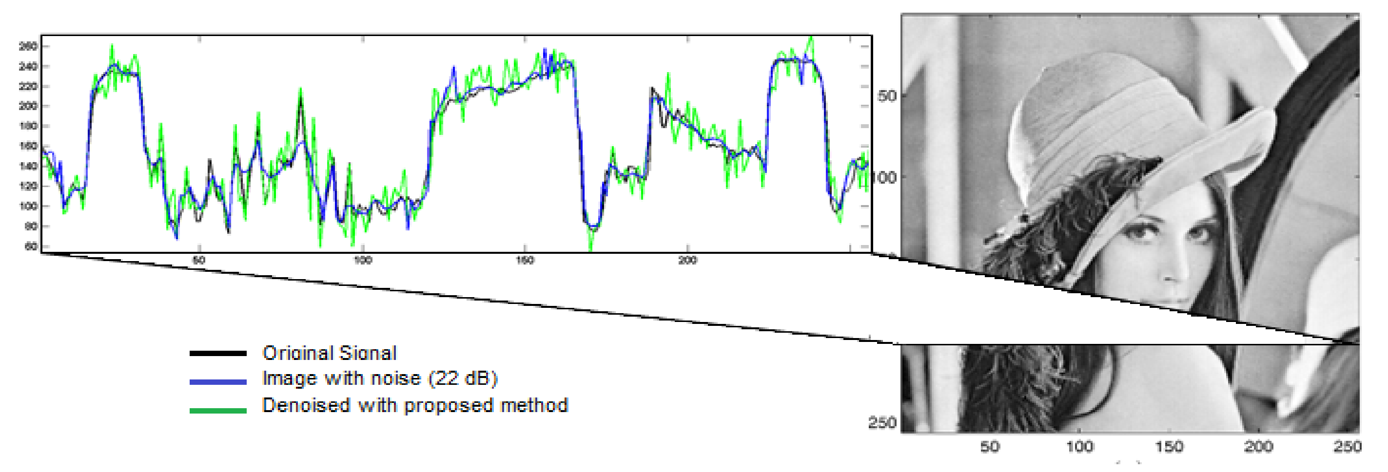
The obtained results in Figure 11c shows that the noise level has reduced and preserved the image structures without introducing spurious oscillations. To illustrate the results of denoising more precisely, we show in Figure 12 and Figure 13, a single row (200) of House and Lena image with noise (22.11 dB white Gaussian noise), plotted as a curve. It can be seen from the figure that the method has filtered most of the noise elements while preserving the edge points. The sharpness and magnitude of these edges were not altered during denoising and the noise elements were removed from the homogeneous regions. The results in Figure 13 also illustrate that the sharp transition or edges (near to step function or discontinuity), are equally preserved and hence the main information about the structure of the image remain unchanged.
We performed the multi scale analysis based splitting and heuristic approach for the reconstruction of House, Lena, circuit, Pepper and Hand images. We generated noisy data from clean image by adding pseudo random numbers (Gaussian White noise) with different peak signal to noise ration (PSNR), the qualitative analysis of the method on both images is summarized in Table 1. We observed improvement of ≈5 at the lowest sigma and relatively better results at high variance of noise with the ≈10 improvement in PSNR in House and ≈8 in the case of Lena image. Figure 14 shows the corresponding correlation curves with different noise levels (sigma) on House image where cross and circle represent the true values computed by the method.
We observed distant correlation with input at high sigma which gradually reduces with decrease in sigma. We generated noisy data from House image by adding pseudo random numbers (Gaussian White noise) resulting in peak signal to noise ratio (PSNR) of approximately 19 dB. Figure 15b,c presents the image with the addition of Gaussian white noise and the denoising result with the proposed method. The obtained PSNR is 26 dB with Lipschitz based method and also the visual evaluation emphasizes the proposed method has not introduced any spurious edges as highlighted in Figure 1.
Similarly, Figure 16b,c also presents the image with the addition of Gaussian white noise and the denoising result with the proposed method on Lena image. The improved PSNR is 29.82 dB as compared to the input 22 dB. In Figure 17, the method improved the PSNR on the Circuit image to 26.12 dB. The results obtained on the Hand and Pepper images are also shown in Figure 18 and Figure 19. The proposed Lipschitz estimation-based method significantly improved not only the statistical results but also the visual evaluation to emphasize that the proposed method has not introduced any spurious edges.
We compared the results on the Lena test images with other methods, including the SURE LET, Sure Shrink, VisuShrink, and Bivariate shrinkage functions (Table 2), as explained [29]. We noted that the results obtained at higher noise level were comparable and better than those obtained with the other methods from the literature. The obtained results were approximately similar to the SURE LET and Bivariate shrinkage functions and outperformed the SureShrink and VisuShrink methods.
Table 3 and Table 4 present the qualitative analysis in terms of the Structural SIMilarity (SSIM) of the proposed method with the other denoised images obtained from the wavelet-based denoising methods [22]. The SSIM can estimate the similarity index between two images and, therefore, can be viewed as a quality measure of one of the image degraded or altered with the other which is regarded as of perfect quality. We performed analysis on the ‘Lena’ and ‘Peppers’ images. It can be observed that the denoised images obtained better results than the Bishrink and NeighSure method and were competitive to the SURE LET denoising method in terms of SSIM.
We also analyzed the performance of the method using another criterion, which focused only around the edges. At first, we applied a canny edge detector as shown in Figure 20a to highlight strong edges. Then, we applied morphological dilation of 5 × 5 to generate a binary mask as shown in Figure 20b. The Mask represents the dilated binary image of edges, and the estimated error is:
We estimated the error corresponding to the area of the edge points with the SURE LET denoising method with the proposed method based on the splitting of edges as shown in Figure 20, and we observed increased improvement in SNR with both methods with the difference of ≈1 dB.
6. Conclusions
This paper introduced a method to remove the noise from the signals or images during the acquisition phase of theNDT process. The method preserved the edges and transitions that corresponded to the most significant information about the nature of the signals or images while denoising. The algorithm removed the noise in the homogeneous areas but preserved all structures like the edges or corners by computing the Lipschitz exponents estimated from the modulus maxima lines.
It is shown that the Lipschitz estimation of the anatural image lay within a certain range of values even in the presence of noise and also did not change significantly even in the presence of affine deformation. Based on the detection of edges from the modulus maximas, we classified each image into the edge and background pixels—the edges where the intensity changed abruptly preserved their Lipschitz estimation even with the addition of noise.
The statistical results illustrated that the proposed method had improved PSNR and maintained the sharpness of the edges without introducing any artifacts. The Lipschitz estimation can highlight the discontinuities present in the images, and in more practical applications (e.g., NDT, medical applications), it is of extreme importance to localize them. The results are encouraging to further improve this method by working on multi-scale basis and employing practical examples e.g., surface inspection.
Author Contributions
Methodology: B.J.; Z.J.; E.F. and O.L.; project administration: B.J.; Software: B.J. and Z.J.; Supervision: E.F. and O.L. All authors have read and agreed to the published version of the manuscript.
Funding
This research received no external funding.
Conflicts of Interest
The authors declare no conflict of interest.
Appendix A
The complete algorithm follows following steps:
- We assume that the given image specify the model:f is the noise-free signal, and is the white Gaussian noise .
- At first, we applied wavelet transform based multiscale analysis to detect edges using modulus maxima.
- Lipschitz exponents separate edges from noise and background.
- Definition of classes were defined representing edge and background pixels respectively.
- Restoration algorithm. (assuming maximum smoothness).is the minimum root mean square error.
References
- Goyal, B.; Dogra, A.; Agrawal, S.; Sohi, B.; Sharma, A. Image denoising review: From classical to state-of-the-art approaches. Inf. Fusion 2020, 55, 220–244. [Google Scholar] [CrossRef]
- Bruckstein, A.; Lindenbaum, M.; Fischer, M. On gabor contribution to image enhancement. Comput. Methods Programs Biomed. 1994, 27, 1–8. [Google Scholar]
- Malik, J.; Perona, P. Scale space and edge detection using anisotropic diffusion. IEEE Trans. Pattern Anal. 1990, 12, 629–639. [Google Scholar]
- Catté, F.; Lions, P.L.; Morel, J.M.; Coll, T. Image selective smoothing and edge detection by nonlinear diffusion. J. Numer. Anal. 1992, 29, 845–866. [Google Scholar] [CrossRef]
- Hosotani, F.; Inuzuka, Y.; Hasegawa, M.; Hirobayashi, S.; Misawa, T. Image Denoising With Edge-Preserving and Segmentation Based on Mask NHA. IEEE Trans. Image Process. 2015, 24, 6025–6033. [Google Scholar] [CrossRef] [PubMed]
- Yaroslavsky, L. Digital Picture Processing—An Introduction; Springer: Berlin/Heidelberg, Germany, 1985. [Google Scholar]
- Manduchi, R.; Tomasi, C. Bilateral filtering for gray and color images. In Proceedings of the Sixth International Conference on Computer Vision, Bombay, India, 7 January 1998; pp. 839–846. [Google Scholar]
- Chatterjee, P.; Milanfar, P. patch-based near optimal image denoising. IEEE Trans. Image Process. 2012, 21, 1635–1649. [Google Scholar] [CrossRef] [PubMed]
- Walker, J.S.; Chen, Y.J. Image Denoising Using Tree-based Wavelet Subband Correlations and Shrinkage. Opt. Eng. 2000, 39, 2900–2908. [Google Scholar]
- Tessens, L.; Pizurica, A.; Alecu, A.; Munteanu, A.; Philips, W. Context adaptive image denoising through modeling of curvelet domain statistics. J. Electron. Imaging 2008, 17, 033021. [Google Scholar] [CrossRef]
- Taswell, C. Experiments in Wavelet Shrinkage Denoising. J. Comput. Methods Sci. Eng. 2001, 1, 315–326. [Google Scholar] [CrossRef] [Green Version]
- Starck, J.L.; Canduesy, E.J.; Donoho, D.L. The Curvelet Transform for Image Denoising. IEEE Trans. Image Process. 2002, 11, 670–684. [Google Scholar] [CrossRef] [Green Version]
- Pesquet, J.C.; Benyahia, A.B.; Chaux, C. A SURE Approach for Digital Signal/Image Deconvolution Problems. IEEE Trans. Signal Process. 2009, 57, 4616–4632. [Google Scholar] [CrossRef]
- Patil, S.S.; Patil, A.B.; Deshmukh, S.C.; Chavan, M.N. Wavelet Shrinkage Techniques for Images. Int. J. Comput. Appl. 2010, 7, 975–8887. [Google Scholar] [CrossRef]
- Gao, L.; Wang, G.; Liu, J. Image denoising based on edge detection and pre thresholding Wiener filtering of multi-wavelets fusion. Int. J. Wavelets Multiresolut. Inf. Process. 2015, 13, 1550031. [Google Scholar] [CrossRef]
- Buades, A.; Coll, B.; Morel, J.M. On image denoising methods. In Tech. Note, CMLA; Research Center for Applied Maths, Universite Paris-Saclay: Paris, France, 2004; Volume 5. [Google Scholar]
- Buades, A.; Coll, B.; Morel, J.M. A Review of Image Denoising Algorithms, with a New One. Multiscale Model. Simul. 2005, 4, 490–530. [Google Scholar] [CrossRef]
- Seo, H.J.; Chatterjee, P.; Takeda, H.; Milanfar, P. A Comparison of Some State of the Art Image Denoising Methods. In Proceedings of the Conference Record of the Forty-First Asilomar Conference on Signals, Systems and Computers, Pacific Grove, CA, USA, 4–7 November 2007; pp. 518–522. [Google Scholar]
- Blu, T.; Luisier, F. The SURE-LET approach to image denoising. IEEE Trans. Image Process. 2007, 16, 2778–2786. [Google Scholar] [CrossRef] [Green Version]
- Chen, G.Y.; Kegl, B. Image denoising with complex ridgelets. Pattern Recognit. 2007, 40, 578–585. [Google Scholar] [CrossRef]
- Alkinani, M.H.; El-Sakka, M.R. Patch-based models and algorithms for image denoising: A comparative review between patch-based images denoising methods for additive noise reduction. EURASIP J. Image Video Process. 2017, 2017, 58. [Google Scholar] [CrossRef]
- Naveed, K.; Shaukat, B.; Ehsan, S.; Mcdonald-Maier, K.D.; ur Rehman, N. Multiscale image denoising using goodness-of-fit test based on EDF statistics. PLoS ONE 2019, 14, e0216197. [Google Scholar] [CrossRef]
- Bnou, K.; Raghay, S.; Hakim, A. A wavelet denoising approach based on unsupervised learning model. EURASIP J. Adv. Signal Process. 2020, 2020. [Google Scholar] [CrossRef]
- Jain, P.; Tyagi, V. A survey of edge-preserving image denoising methods. Inf. Syst. Front. 2016, 18, 159–170. [Google Scholar] [CrossRef]
- Pizurica, A. Image Denoising Algorithms: From Wavelet Shrinkage to Non-local Collaborative Filtering. Wiley Encycl. Electr. Electron. Eng. 2017, 10. [Google Scholar] [CrossRef]
- Chandrajit Pal, A.C.; Ghosh, R. A Brief Survey of Recent Edge-Preserving Smoothing Algorithms on Digital Images. arXiv 2015, arXiv:1503.07297. [Google Scholar]
- Mallat, S. A Wavelet Tour of Signal Processing, 2nd ed.; Academic Press: Cambridge, MA, USA, 1998. [Google Scholar]
- Grossmann, A.; Morlet, J. Decomposition of Hardy Functions into Square Integrable Wavelets of Constant Shape. SIAM J. Math. Anal. 1984, 15, 723–736. [Google Scholar] [CrossRef]
- Sendur, L.; Selesnick, I.W. Bivariate shrinkage functions for wavelet-based denoising exploiting interscale dependency. IEEE Trans. Signal Process. 2002, 50, 2744–2756. [Google Scholar] [CrossRef] [Green Version]
Figure 1.
(a) An edge of House Image, (b) Image with Gaussian white noise (Input PSNR = 18.59 dB), (c) After Denoising (PSNR = 28.77 dB).
Figure 1.
(a) An edge of House Image, (b) Image with Gaussian white noise (Input PSNR = 18.59 dB), (c) After Denoising (PSNR = 28.77 dB).

Figure 2.
Block diagram of the method.

Figure 3.
The continuous wavelet transform (CWT)-based multi scale decomposition of the image with corresponding to the Gaussian function. (a) Images correspond to the gradient image in the vertical direction measuring changes in intensity where as the (b) images represent a gradient image in the horizontal direction measuring the horizontal change in intensity. (c) Wavelet transform modulus maxima representing significant transitions or edges in the images and (d) shows the angle of these transitions.

Figure 4.
(a) House image, modulus maxima: (b) before thresholding, (c) after thresholding.

Figure 5.
Consent of Modulus maxima lines. Local maxima search for the closest phase maxima in the next scale.
Figure 5.
Consent of Modulus maxima lines. Local maxima search for the closest phase maxima in the next scale.

Figure 6.
(a) Original Lena image, (b) modulus maxima after thresholding, (c) histogram of Lipschitz exponents correspond to maxima lines in (b).
Figure 6.
(a) Original Lena image, (b) modulus maxima after thresholding, (c) histogram of Lipschitz exponents correspond to maxima lines in (b).

Figure 7.
(a) Original House image, (b) modulus maxima after thresholding, (c) histogram of Lipschitz exponents correspond to maxima lines in (b).
Figure 7.
(a) Original House image, (b) modulus maxima after thresholding, (c) histogram of Lipschitz exponents correspond to maxima lines in (b).

Figure 8.
(a) Concept of two classes. Class 1 belongs to the edges and Class 2 belongs to the background. (b) Neighborhood contribution.
Figure 8.
(a) Concept of two classes. Class 1 belongs to the edges and Class 2 belongs to the background. (b) Neighborhood contribution.

Figure 9.
(a) Row No. 125 of image shown in Figure 2a, (b) Row No. 125 of the image with the addition if Gaussian noise (28 dB) modulus maxima are marked as a circle in both images, and the corresponding Lipschitz value is written in numerical form.
Figure 9.
(a) Row No. 125 of image shown in Figure 2a, (b) Row No. 125 of the image with the addition if Gaussian noise (28 dB) modulus maxima are marked as a circle in both images, and the corresponding Lipschitz value is written in numerical form.

Figure 10.
(a) Rotated Lena image (10 of rotation), (b) Modulus maxima lines after thresholding, (c) Histogram of Lipschitz Values.
Figure 10.
(a) Rotated Lena image (10 of rotation), (b) Modulus maxima lines after thresholding, (c) Histogram of Lipschitz Values.

Figure 11.
(a) House Image, (b) House Image with Gaussian white noise (Input PSNR = 24.59 dB), (c) Denoised Image with proposed Method (29.14 dB).
Figure 11.
(a) House Image, (b) House Image with Gaussian white noise (Input PSNR = 24.59 dB), (c) Denoised Image with proposed Method (29.14 dB).

Figure 12.
Row 200 of Image, with Gaussian white noise (Input PSNR = 22.11 dB) and denoised with proposed Method (27.93 dB).
Figure 12.
Row 200 of Image, with Gaussian white noise (Input PSNR = 22.11 dB) and denoised with proposed Method (27.93 dB).

Figure 13.
Row 200 of Lena Image, row with Gaussian white noise (Input PSNR = 22.11 dB) and Denoised row with SSplit Method (27.77 dB).
Figure 13.
Row 200 of Lena Image, row with Gaussian white noise (Input PSNR = 22.11 dB) and Denoised row with SSplit Method (27.77 dB).

Figure 14.
Correlation results with different noise levels.

Figure 15.
(a) Original Image, (b) Image with the addition of Gaussian white noise (Input PSNR = 18.59 dB), (c) Denoising with proposed method (Output PSNR = 26.82 dB).
Figure 15.
(a) Original Image, (b) Image with the addition of Gaussian white noise (Input PSNR = 18.59 dB), (c) Denoising with proposed method (Output PSNR = 26.82 dB).

Figure 16.
(a) Original image, (b) Image with the addition of Gaussian white noise (Input PSNR = 22.11 dB), (c) Denoising with proposed method (Output PSNR = 29.82 dB).
Figure 16.
(a) Original image, (b) Image with the addition of Gaussian white noise (Input PSNR = 22.11 dB), (c) Denoising with proposed method (Output PSNR = 29.82 dB).

Figure 17.
(a) Original image, (b) Image with the addition of Gaussian white noise (Input PSNR = 22.11 dB), (c) Denoising with proposed method (Output PSNR = 26.12 dB).
Figure 17.
(a) Original image, (b) Image with the addition of Gaussian white noise (Input PSNR = 22.11 dB), (c) Denoising with proposed method (Output PSNR = 26.12 dB).

Figure 18.
(a) Original image, (b) Image with the addition of Gaussian white noise (Input PSNR = 19.27 dB), (c) Denoising with proposed method (Output PSNR = 26.42 dB).
Figure 18.
(a) Original image, (b) Image with the addition of Gaussian white noise (Input PSNR = 19.27 dB), (c) Denoising with proposed method (Output PSNR = 26.42 dB).

Figure 19.
(a) Original image, (b) Image with the addition of Gaussian white noise (Input PSNR = 18.59 dB), (c) Denoising with proposed method (Output PSNR = 24.59 dB).
Figure 19.
(a) Original image, (b) Image with the addition of Gaussian white noise (Input PSNR = 18.59 dB), (c) Denoising with proposed method (Output PSNR = 24.59 dB).

Figure 20.
(a) Binary image, (b) Dilated image with the addition of Gaussian white noise (Input PSNR = 18.59 dB), (c) SURE-LET method (Output PSNR = 32.21 dB), (d) SSplit method (Output PSNR = 33.23 dB).
Figure 20.
(a) Binary image, (b) Dilated image with the addition of Gaussian white noise (Input PSNR = 18.59 dB), (c) SURE-LET method (Output PSNR = 32.21 dB), (d) SSplit method (Output PSNR = 33.23 dB).


Table 1.
Obtained results on House, Lena, Pepper and Hand image with different noise levels (PSNR).
| House | Lena | ||||||
|---|---|---|---|---|---|---|---|
| Sigma | Input (dB) | SSplit (dB) | Δ | Sigma | Input (dB) | SSplit (dB) | Δ |
| 15 | 24.61 | 31.50 | ≈6 | 15 | 24.61 | 32.08 | ≈7 |
| 20 | 22.11 | 29.93 | ≈7 | 20 | 22.11 | 30.80 | ≈8 |
| 25 | 20.17 | 29.09 | ≈8 | 25 | 20.17 | 29.98 | ≈9 |
| 30 | 18.59 | 28.89 | ≈10 | 30 | 18.59 | 29.09 | ≈10 |
| 35 | 17.25 | 27.85 | ≈10 | 35 | 17.25 | 28.43 | ≈11 |
| Pepper | Hand | ||||||
| Sigma | Input (dB) | SSplit (dB) | Δ | Sigma | Input (dB) | SSplit (dB) | Δ |
| 15 | 24.61 | 29.34 | ≈5 | 15 | 24.61 | 28.77 | ≈4 |
| 20 | 22.11 | 29.53 | ≈7 | 20 | 22.11 | 28.13 | ≈6 |
| 25 | 20.17 | 28.89 | ≈8 | 25 | 20.17 | 27.74 | ≈7 |
| 30 | 18.59 | 28.79 | ≈9 | 30 | 18.59 | 27.13 | ≈8 |
| 35 | 17.25 | 28.05 | ≈10 | 35 | 17.25 | 26.39 | ≈9 |
Table 2.
PSNR values for Lena test images with different noise levels and denoised with: the SURE LET, SureShrink, VisuShrink, Bivariate shrinkage function, and SSplit methods.
Table 2.
PSNR values for Lena test images with different noise levels and denoised with: the SURE LET, SureShrink, VisuShrink, Bivariate shrinkage function, and SSplit methods.
| Sigma | Input (dB) | SURE-LET (dB) | Sureshrink | Visu Shrink | Bivariate Shrinkage | SSplit (dB) |
|---|---|---|---|---|---|---|
| 15 | 24.65 | 32.17 | 31.59 | 27.48 | 32.06 | 32.08 |
| 20 | 22.14 | 30.94 | 30.22 | 26.46 | 30.73 | 30.81 |
| 25 | 20.17 | 30.03 | 29.14 | 25.67 | 29.81 | 29.97 |
| 30 | 18.62 | 29.32 | 28.38 | 25.14 | 28.94 | 29.11 |
Table 3.
Comparison of the proposed methods with the other wavelet-based image denoising methods on the ‘Lena’ image in terms of the structural similarity (SSIM) for a range of input noise levels = 10 to = 50 [22].
Table 3.
Comparison of the proposed methods with the other wavelet-based image denoising methods on the ‘Lena’ image in terms of the structural similarity (SSIM) for a range of input noise levels = 10 to = 50 [22].
| Sigma | Input | SURE-LET | Bishrink | NeighSure | SSplit |
|---|---|---|---|---|---|
| 10 | 0.53 | 0.66 | 0.58 | 0.60 | 0.63 |
| 20 | 0.34 | 0.53 | 0.47 | 0.50 | 0.58 |
| 30 | 0.246 | 0.46 | 0.42 | 0.43 | 0.45 |
| 40 | 0.18 | 0.414 | 0.37 | 0.39 | 0.41 |
| 50 | 0.14 | 0.37 | 0.33 | 0.35 | 0.36 |
Table 4.
Comparison of the proposed methods with the other wavelet-based image denoising methods on the ‘Pepper’ image in terms of the structural similarity (SSIM) for a range of input noise levels = 10 to = 50 [22].
Table 4.
Comparison of the proposed methods with the other wavelet-based image denoising methods on the ‘Pepper’ image in terms of the structural similarity (SSIM) for a range of input noise levels = 10 to = 50 [22].
| Sigma | Input | SURE-LET | Bishrink | NeighSure | SSplit |
|---|---|---|---|---|---|
| 10 | 0.56 | 0.73 | 0.49 | 0.57 | 0.69 |
| 20 | 0.37 | 0.61 | 0.41 | 0.43 | 0.58 |
| 30 | 0.27 | 0.54 | 0.37 | 0.38 | 0.53 |
| 40 | 0.21 | 0.49 | 0.33 | 0.35 | 0.44 |
| 50 | 0.16 | 0.44 | 0.31 | 0.32 | 0.42 |
Publisher’s Note: MDPI stays neutral with regard to jurisdictional claims in published maps and institutional affiliations. |
© 2021 by the authors. Licensee MDPI, Basel, Switzerland. This article is an open access article distributed under the terms and conditions of the Creative Commons Attribution (CC BY) license (https://creativecommons.org/licenses/by/4.0/).
Share and Cite
MDPI and ACS Style
Jalil, B.; Jalil, Z.; Fauvet, E.; Laligant, O. Edge-Preserving Image Denoising Based on Lipschitz Estimation. Appl. Sci. 2021, 11, 5126. https://0-doi-org.brum.beds.ac.uk/10.3390/app11115126
AMA Style
Jalil B, Jalil Z, Fauvet E, Laligant O. Edge-Preserving Image Denoising Based on Lipschitz Estimation. Applied Sciences. 2021; 11(11):5126. https://0-doi-org.brum.beds.ac.uk/10.3390/app11115126
Chicago/Turabian StyleJalil, Bushra, Zunera Jalil, Eric Fauvet, and Olivier Laligant. 2021. "Edge-Preserving Image Denoising Based on Lipschitz Estimation" Applied Sciences 11, no. 11: 5126. https://0-doi-org.brum.beds.ac.uk/10.3390/app11115126
Note that from the first issue of 2016, this journal uses article numbers instead of page numbers. See further details here.