
VBM-Based Alzheimer’s Disease Detection from the Region of Interest of T1 MRI with Supportive Gaussian Smoothing and a Bayesian Regularized Neural Network

 , , and
Abstract
:1. Introduction
2. Materials
2.1. Image Acquisition
2.2. Participants
3. Methodology
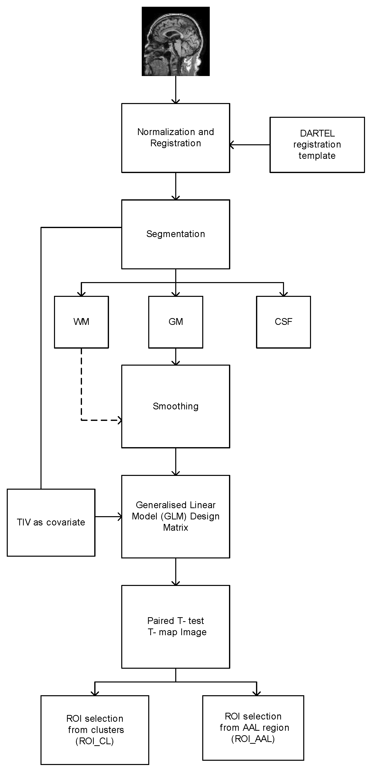
3.1. VBM SPM Model
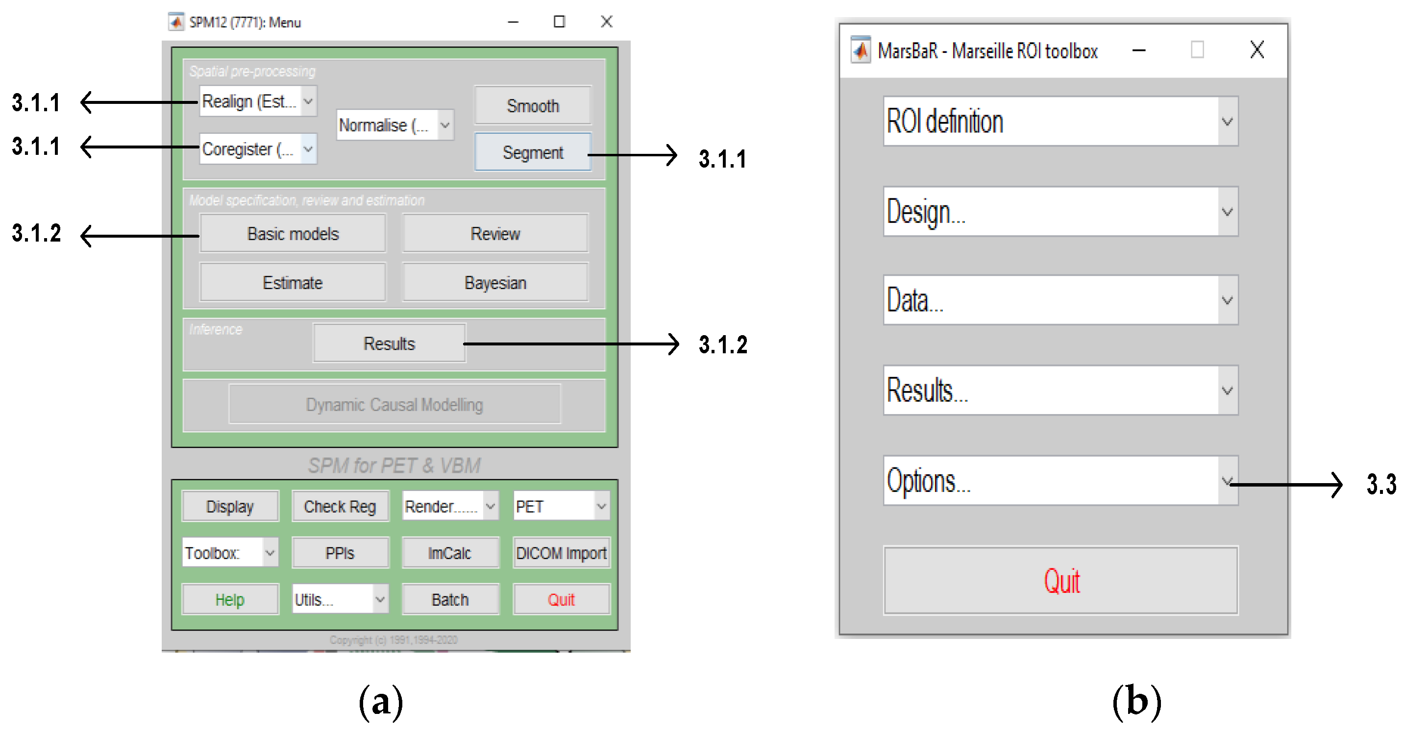
3.1.1. MRI Preprocessing for Voxel-Based Model
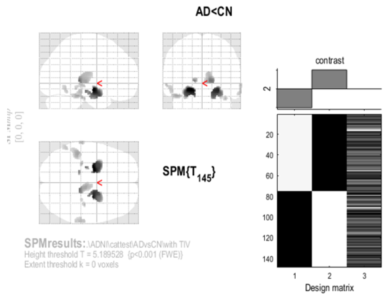
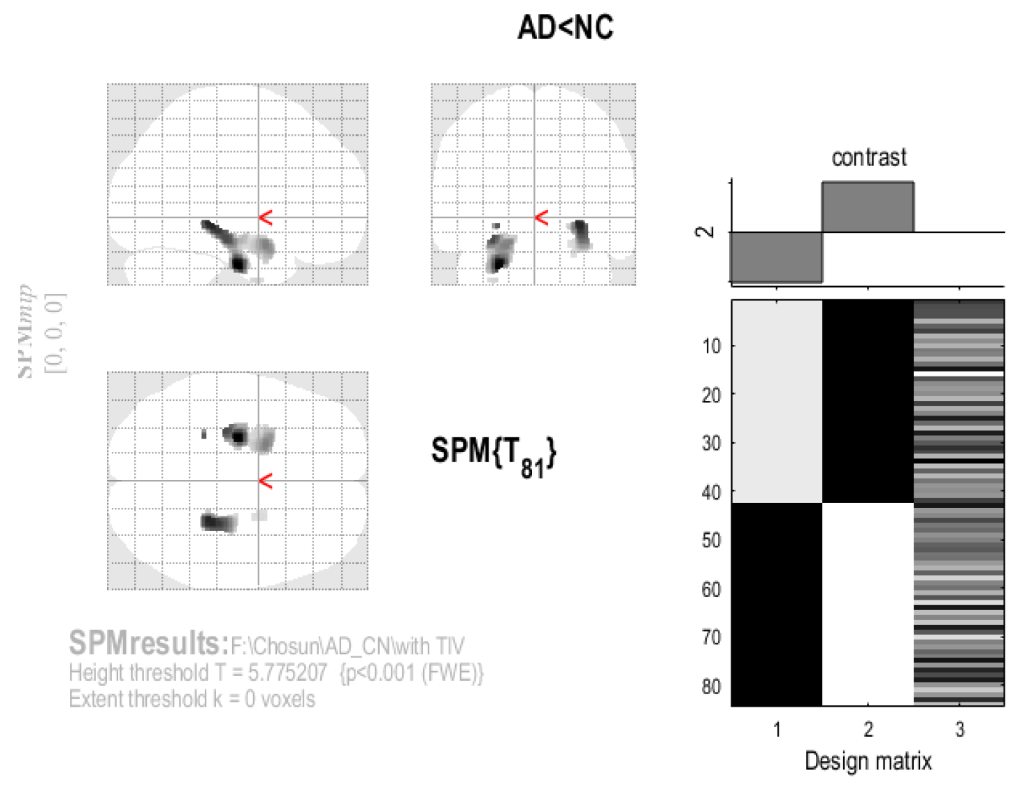
3.1.2. SPM t-Map
3.2. ROI Selection
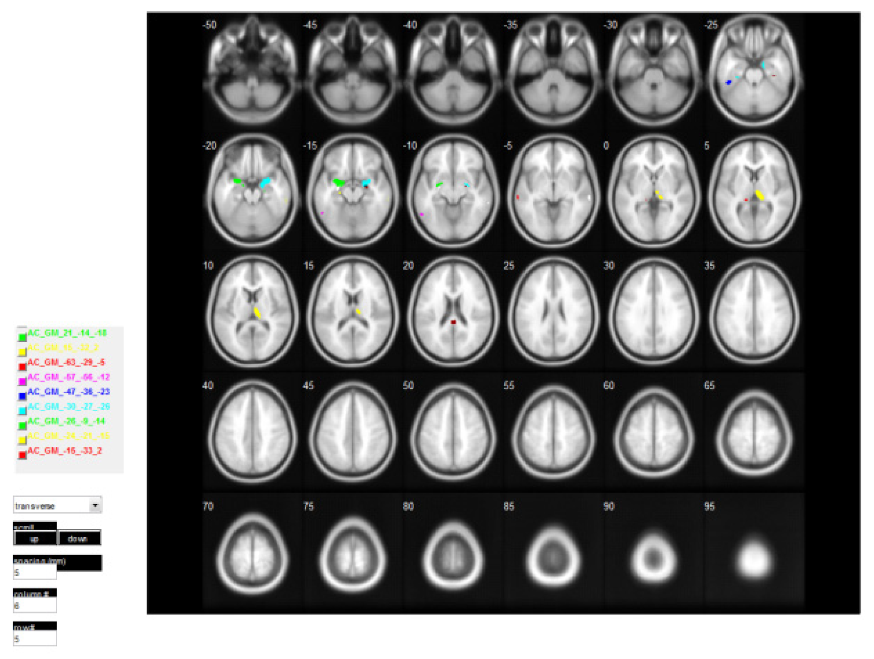
3.2.1. From Each Cluster Generated into Separate ROI
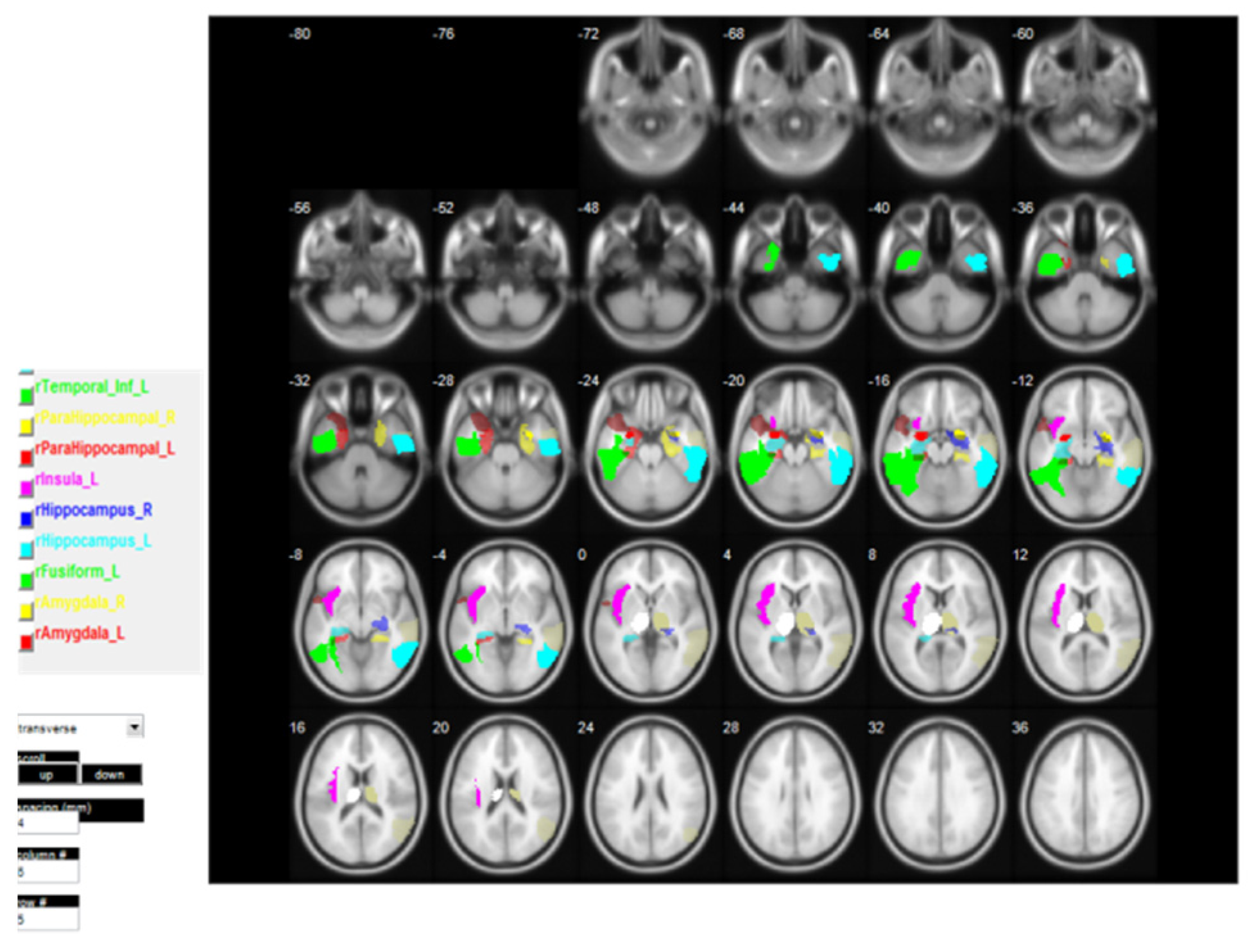
3.2.2. From AAL Template Based on the Anatomic Region
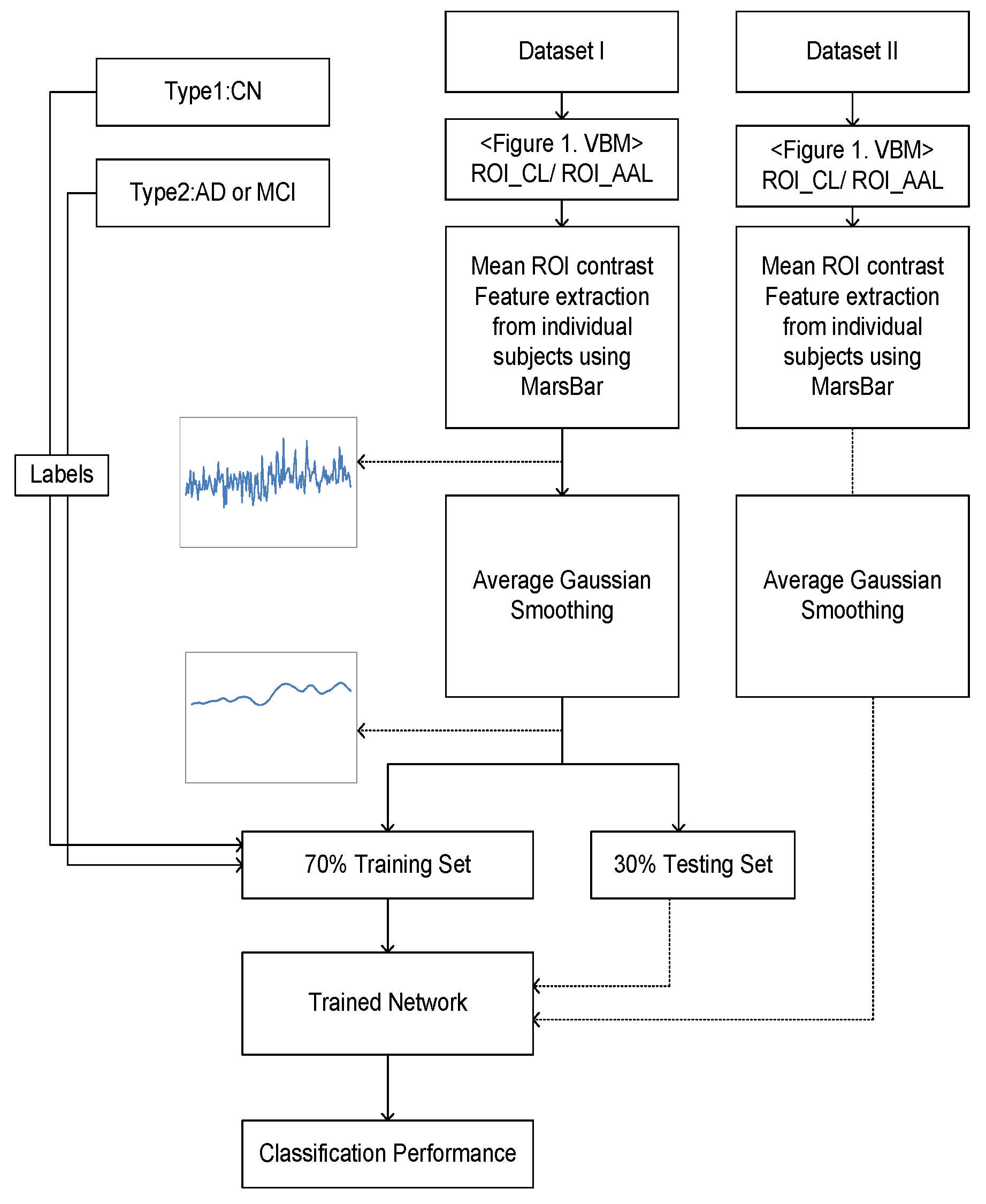
3.3. Feature Extraction from Both Types of ROIs
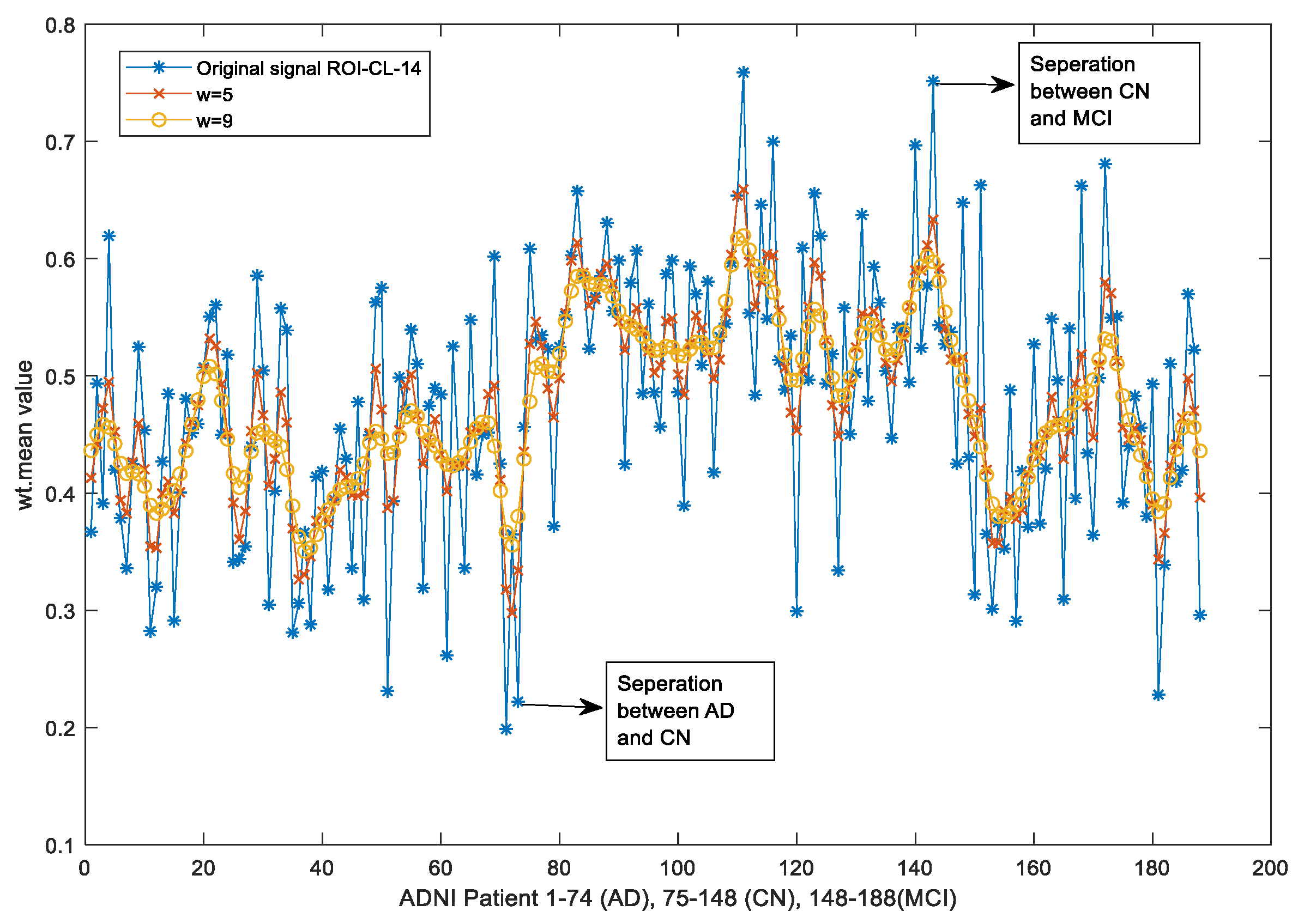
4. Gaussian Smoothing
5. Bayesian Regularized Feed-Forward Neural Network (BR–FNN)
6. Performance and Discussion
6.1. ROI Selection and Its Importance
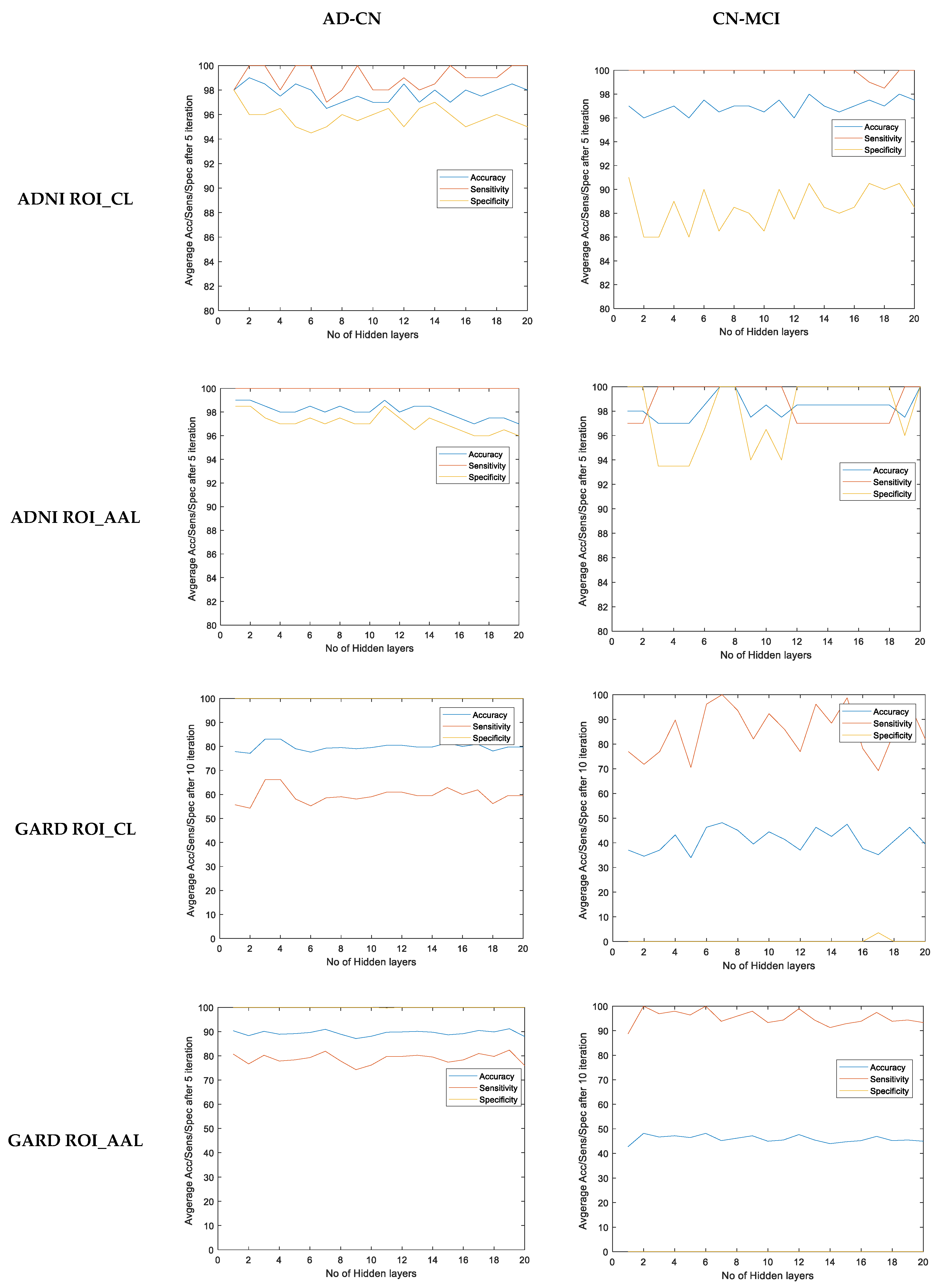
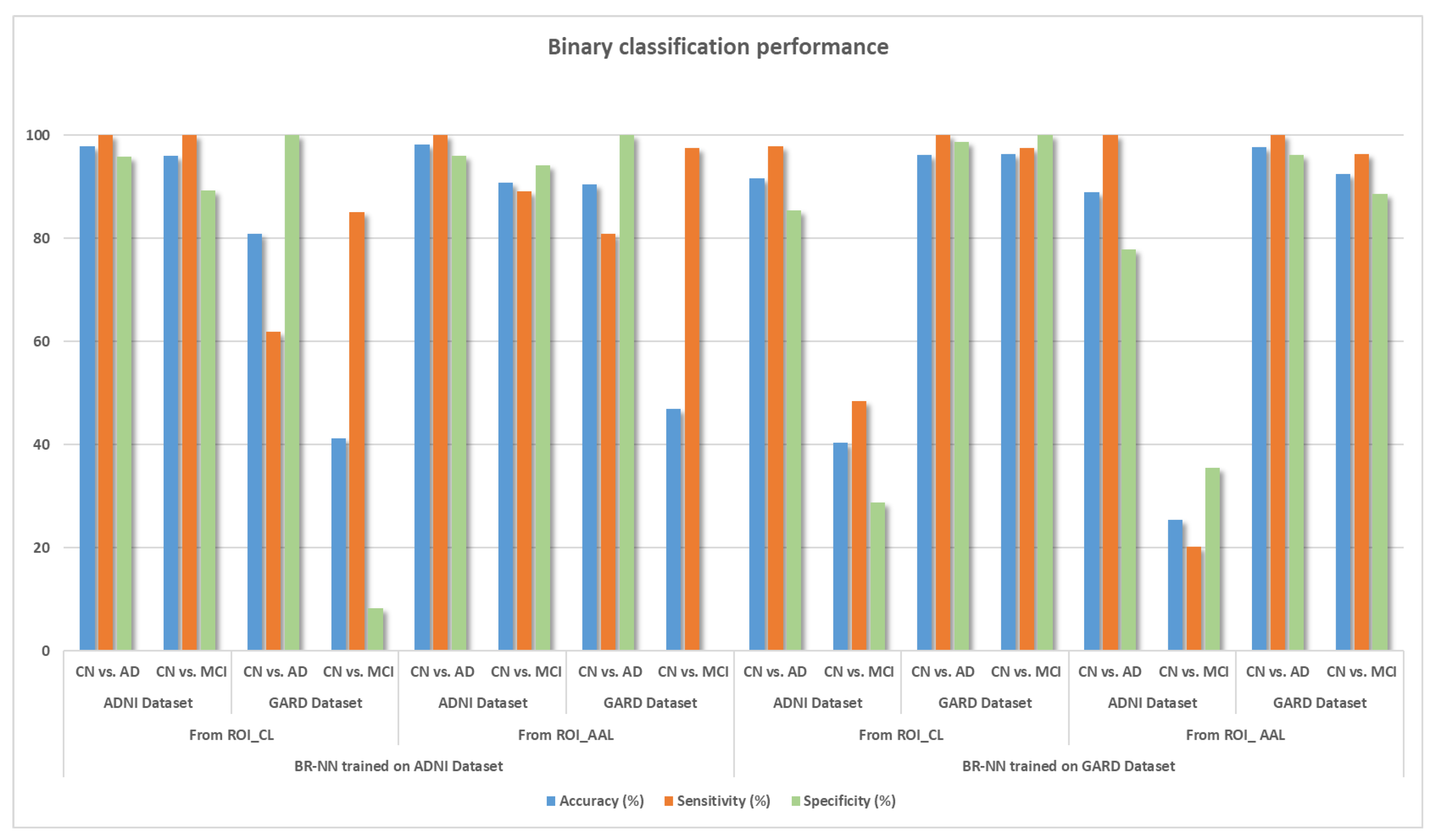
6.2. Experimental Result
6.3. Discussion
6.4. Comparison with State-of-the-Art Performance
7. Conclusions
Supplementary Materials
Author Contributions
Funding
Institutional Review Board Statement
Informed Consent Statement
Data Availability Statement
Acknowledgments
Conflicts of Interest
Ethics Statement
Appendix A

| MR1 | 0.3093 | 0.2374 | 0.3281 | 0.2701 | 0.3236 | 0.2851 | 0.3153 | 0.4931 | 0.3490 | 0.3527 | 0.3216 | 0.3242 | 0.3461 | 0.3991 | 0.1228 | 0.2657 | 0.3673 | 0.3670 | AD |
| MR2 | 0.3925 | 0.5445 | 0.4526 | 0.5315 | 0.3892 | 0.4626 | 0.3869 | 0.4416 | 0.5676 | 0.4565 | 0.5105 | 0.4238 | 0.3969 | 0.3980 | 0.1114 | 0.5032 | 0.3712 | 0.4937 | AD |
| MR3 | 0.3253 | 0.3617 | 0.3490 | 0.3129 | 0.4553 | 0.4456 | 0.4495 | 0.3161 | 0.4353 | 0.3725 | 0.3614 | 0.3375 | 0.3813 | 0.3794 | 0.1176 | 0.3147 | 0.3229 | 0.3914 | AD |
| MR75 | 0.5074 | 0.5122 | 0.5295 | 0.5587 | 0.4627 | 0.5046 | 0.4328 | 0.5831 | 0.6103 | 0.5532 | 0.5588 | 0.4860 | 0.4192 | 0.4568 | 0.1192 | 0.5566 | 0.4118 | 0.6085 | CN |
| MR76 | 0.4533 | 0.4398 | 0.4810 | 0.4092 | 0.5092 | 0.4700 | 0.4434 | 0.5087 | 0.5012 | 0.5178 | 0.4451 | 0.4844 | 0.4669 | 0.5073 | 0.1567 | 0.4826 | 0.3516 | 0.5306 | CN |
| MR77 | 0.5358 | 0.4974 | 0.4879 | 0.5012 | 0.4016 | 0.3805 | 0.3538 | 0.5088 | 0.6036 | 0.5197 | 0.4281 | 0.3673 | 0.3385 | 0.3621 | 0.1126 | 0.4999 | 0.4863 | 0.5348 | CN |
| MR149 | 0.2897 | 0.4256 | 0.4016 | 0.4596 | 0.4078 | 0.3795 | 0.3595 | 0.4271 | 0.4182 | 0.4126 | 0.4333 | 0.3582 | 0.2984 | 0.3184 | 0.0808 | 0.3981 | 0.2601 | 0.4306 | MCI |
| MR150 | 0.2912 | 0.3234 | 0.4049 | 0.4397 | 0.3846 | 0.3320 | 0.2157 | 0.4364 | 0.4046 | 0.3805 | 0.4556 | 0.5041 | 0.1985 | 0.3619 | 0.0941 | 0.3287 | 0.3490 | 0.3135 | MCI |
| MR151 | 0.3904 | 0.6184 | 0.4838 | 0.4348 | 0.3609 | 0.3279 | 0.3592 | 0.5221 | 0.7012 | 0.6146 | 0.5170 | 0.4805 | 0.3935 | 0.3767 | 0.1603 | 0.5817 | 0.4235 | 0.6626 | MCI |
| Location/ | AC_GM cluster at [−15.0 −33.0 1.5] | AC_GM cluster at [−24.0 −21.0 −15.0] | AC_GM cluster at [−25.5 −9.0 −13.5] | AC_GM cluster at [−30.0 −27.0 −25.5] | AC_GM cluster at [−46.5 −36.0 −22.5] | AC_GM cluster at [−57.0 −55.5 −12.0] | AC_GM cluster at [−63.0 −28.5 −4.5] | AC_GM cluster at [15.0 −31.5 1.5] | AC_GM cluster at [21.0 −13.5 −18.0] | AC_GM cluster at [25.5 −9.0 −13.5] | AC_GM cluster at [30.0 −27.0 −25.5] | AC_GM cluster at [37.5 −22.5 −27.0] | AC_GM cluster at [64.5 −24.0 −6.0] | AC_GM cluster at [64.5 −31.5 −16.5] | AC_WM cluster at [1.5 −36.0 21.0] | CM_GM cluster at [−27.0 −10.5 −13.5] | CM_GM cluster at [13.5 −31.5 1.5] | CM_GM cluster at [27.0 −9.0 −15.0] | Target class/Label |
| MR1 | 0.3063 | 0.3209 | 0.2122 | 0.1769 | 0.2674 | 0.3203 | 0.2141 | 0.2677 | 0.2654 | 0.2794 | 0.2672 | 0.2041 | 0.3475 | 0.3533 | AD |
| MR2 | 0.4729 | 0.3926 | 0.3446 | 0.3796 | 0.3473 | 0.4205 | 0.4001 | 0.3818 | 0.3550 | 0.3068 | 0.3186 | 0.2946 | 0.3656 | 0.3195 | AD |
| MR3 | 0.3469 | 0.3264 | 0.2977 | 0.2506 | 0.2616 | 0.3823 | 0.2678 | 0.3069 | 0.3429 | 0.3112 | 0.3060 | 0.2353 | 0.2274 | 0.2357 | AD |
| MR75 | 0.5721 | 0.4882 | 0.3812 | 0.3908 | 0.4046 | 0.4206 | 0.4166 | 0.4157 | 0.3927 | 0.3580 | 0.3530 | 0.3380 | 0.4459 | 0.4360 | CN |
| MR76 | 0.5252 | 0.4617 | 0.3808 | 0.3626 | 0.3669 | 0.3988 | 0.3864 | 0.3987 | 0.4061 | 0.3820 | 0.3699 | 0.3246 | 0.3908 | 0.3738 | CN |
| MR77 | 0.5287 | 0.4413 | 0.3150 | 0.3775 | 0.3726 | 0.4020 | 0.4223 | 0.4084 | 0.2933 | 0.2943 | 0.2772 | 0.3368 | 0.3458 | 0.3355 | CN |
| MR149 | 0.4055 | 0.3584 | 0.2730 | 0.3055 | 0.2877 | 0.3131 | 0.3126 | 0.3173 | 0.2794 | 0.2640 | 0.2800 | 0.2409 | 0.3247 | 0.3313 | MCI |
| MR150 | 0.4358 | 0.3292 | 0.2948 | 0.2669 | 0.2827 | 0.3610 | 0.4250 | 0.4012 | 0.3014 | 0.2882 | 0.2119 | 0.4619 | 0.2773 | 0.2914 | MCI |
| MR151 | 0.5278 | 0.5028 | 0.3238 | 0.4351 | 0.4315 | 0.4136 | 0.4195 | 0.4683 | 0.3103 | 0.3312 | 0.3073 | 0.2985 | 0.4123 | 0.4060 | MCI |
| Location | rAmygdala_L_f_img | rAmygdala_R_f_img | rFusiform_L_f_img | rHippocampus_L_f_img | rHippocampus_R_f_img | rInsula_L_f_img | rParaHippocampal_L_f_img | rParaHippocampal_R_f_img | rTemporal_Inf_L_f_img | rTemporal_Inf_R_f_img | rTemporal_Mid_R_f_img | rTemporal_Pole_Sup_L_f_img | rThalamus_L_f_img | rThalamus_R_f_img | Target class/Label |
| Test Condition | Features | BR-NN Hidden Layer=17 | Iteration 1 | Iteration 2 | Iteration 3 | Iteration 4 | Iteration 5 | Iteration 6 | Iteration 7 | Iteration 8 | Iteration 9 | Iteration 10 |
|---|---|---|---|---|---|---|---|---|---|---|---|---|
| AD vs. CN | ROI_CL | Validation (ADNI 30%) | [0.97 1 0.95] | [1 1 1] | [1 1 1] | [0.97 1 0.96] | [1 1 1] | [1 1 1] | [1 1 1] | [1 1 1] | [0.98 1 0.94] | [0.98 1 0.93] |
| Testing (GARD 100%) | [0.80 0.61 1] | [ 0.82 0.64 1] | [0.77 0.54 1] | [0.83 0.66 1] | [0.78 0.57 1] | [0.91 0.83 1] | [0.91 0.83 1] | [0.78 0.57 1] | [0.83 0.66 1] | [0.80 0.61 1] | ||
| ROI_AAL | Validation (ADNI 30%) | [1 1 1] | [1 1 1] | [1 1 1] | [1 1 1] | [0.97 1 0.95] | [1 1 1] | [1 1 1] | [1 1 1] | [0.95 1 0.90] | [0.97 1 0.95] | |
| Testing (GARD 100%) | [0.84 0.69 1] | [0.88 0.76 1] | [0.90 0.80 1] | [0.85 0.71 1] | [0.89 0.78 1] | [0.97 0.95 1] | [0.94 0.88 1] | [0.96 0.92] | [0.88 0.76 1] | [0.85 0.71 1] | ||
| CN vs. MCI | ROI_CL | Validation (ADNI 30%) | [1 1 1] | [0.97 1 0.91] | [1 1 1] | [1 1 1] | [1 1 1] | [0.91 1 0.84] | [1 1 1] | [1 1 1] | [1 1 1] | [0.94 0.91 1] |
| Testing (GARD 100%) | [0.39 0.82 0] | [0.48 1 0] | [0.38 0.79 0] | [0.44 0.92 0] | [0.48 1 0] | [0.38 0.79 0] | [0.39 0.82 0] | [0.46 0.97 0] | [0.48 1 0] | [0.41 0.87 0] | ||
| ROI_AAL | Validation (ADNI 30%) | [1 1 1] | [0.94 1 0.875 | [1 1 1] | [1 1 1] | [0.94 1 0.85] | [1 1 1] | [1 1 1] | [1 1 1] | [0.97 1 0.92] | [0.97 1 0.92] | |
| Testing (GARD 100%) | [0.43 0.89 0] | [0.44 0.92 0] | [0.43 0.89 0] | [0.41 0.87 0] | [0.48 1 0] | [0.40 0.84 0] | [0.40 0.84 0] | [0.46 0.97 0] | [0.35 0.74 0] | [0.29 0.61 0] |
References
- Guo, H.; Zhang, F.; Chen, J.; Xu, Y.; Xiang, J. Machine Learning Classification Combining Multiple Features of a Hyper-Network of fMRI Data in Alzheimer’s Disease. Front. Neurosci. Orig. Res. 2017, 11, 615. [Google Scholar] [CrossRef]
- Cuingnet, R.; Gerardin, E.; Tessieras, J.; Auzias, G.; Lehéricy, S.; Habert, M.O.; Chupin, M.; Benali, H.; Colliot, O.; Alzheimer’s Disease Neuroimaging Initiative. Automatic classification of patients with Alzheimer’s disease from structural MRI: A comparison of ten methods using the ADNI database. NeuroImage 2011, 56, 766–781. [Google Scholar] [CrossRef] [PubMed] [Green Version]
- Ashburner, J.; Friston, K.J. Voxel-Based Morphometry—The Methods. NeuroImage 2000, 11, 805–821. [Google Scholar] [CrossRef] [Green Version]
- Savio, A.; Sebastian, M.G.; Chyzyk, D.; Hernandez, C.; Graña, M.; Sistiaga, A.; de Munain, A.L.; Villanua, J. Neurocognitive disorder detection based on feature vectors extracted from VBM analysis of structural MRI. Comput. Biol. Med. 2011, 41, 600–610. [Google Scholar] [CrossRef] [PubMed]
- Busatto, G.E.; Garrido, G.E.J.; Almeida, O.P.; Castro, C.C.; Camargo, C.H.; Cid, C.G.; Buchpiguel, C.A.; Furuie, S.; Bottino, C.M. A voxel-based morphometry study of temporal lobe gray matter reductions in Alzheimer’s disease. Neurobiol. Aging 2003, 24, 221–231. [Google Scholar] [CrossRef]
- Frisoni, G.B.; Testa, C.; Zorzan, A.; Sabattoli, F.; Beltramello, A.; Soininen, H.; Laakso, M.P. Detection of grey matter loss in mild Alzheimer’s disease with voxel based Morphometry Journal of Neurology. Neurosurg. Psychiatry 2002, 73, 657–664. [Google Scholar] [CrossRef] [Green Version]
- Beheshti, I.; Demirel, H. Probability distribution function-based classification of structural MRI for the detection of Alzheimer’s disease. Comput. Biol. Med. 2015, 64, 208–216. [Google Scholar] [CrossRef] [PubMed]
- Beheshti, I.; Demirel, H.; Farokhian, F.; Yang, C.; Matsuda, H. Structural MRI-based detection of Alzheimer’s disease using feature ranking and classification error. Comput. Methods Programs Biomed. 2016, 137, 177–193. [Google Scholar] [CrossRef]
- Jha, D.; Kim, J.I.; Kwon, G.R. Diagnosis of Alzheimer’s disease using dual-tree complex wavelet transform, PCA, and feed-forward neural network. J. Healthc. Eng. 2017, 2017, 9060124. [Google Scholar] [CrossRef]
- Wang, S.H.; Zhang, Y.; Li, Y.; Jia, W.; Yang, W.; Zhang, Y. Single slice based detection for Alzheimer’s disease via wavelet entropy and multilayer perceptron trained by biogeography-based optimization. Multimed. Tools Appl. 2016, 77, 10393–10417. [Google Scholar] [CrossRef]
- Zhang, Y.; Wang, S.; Dong, Z. Classification of Alzheimer disease based on structural magnetic resonance imaging by kernel uspport vector machine decision tree. Prog. Electromagn. Res. 2014, 144, 171–184. [Google Scholar] [CrossRef] [Green Version]
- Zhang, Y.; Wu, L.; Wang, S. Magnetic resonance brain image classification by an improved artificial bee colony algorithm. Prog. Electromagn. Res. 2011, 116, 65–79. [Google Scholar] [CrossRef] [Green Version]
- Neffati, S.; Ben Abdellafou, K.; Jaffel, I.; Taouali, O.; Bouzrara, K. An improved machine learning technique based on downsized KPCA for Alzheimer’s disease classification. Int. J. Imaging Syst. Technol. 2018, 29, 121–131. [Google Scholar] [CrossRef]
- Suk, H.; Lee, S.W.; Shen, D. Hierarchical feature representation and multimodal fusion with deep learning for AD/MCI diagnosis. NeuroImage 2014, 101, 569–582. [Google Scholar] [CrossRef] [Green Version]
- Amoroso, N.; Diacono, D.; Fanizzi, A.; La Rocca, M.; Monaco, A.; Lombardi, A.; Guaragnella, C.; Bellotti, R.; Tangaro, S. Deep learning reveals Alzheimer’s disease onset in MCI subjects: Results from an international challenge. J. Neurosci. Methods 2018, 302, 3–9. [Google Scholar] [CrossRef] [Green Version]
- Khagi, B.; Kwon, G.R.; Lama, R. Comparative analysis of Alzheimer’s disease classification by CDR level using CNN, feature selection, and machine-learning techniques. Int. J. Imaging Syst. Technol. 2019, 29, 297–310. [Google Scholar] [CrossRef]
- Shuai, B.; Zuo, Z.; Wang, B.; Wang, G. Dag-recurrent neural networks for scene labeling. In Proceedings of the IEEE Conference on Computer Vision and Pattern Recognition, Las Vegas, NV, USA, 27–30 June 2016; pp. 3620–3629. [Google Scholar]
- Yu, L.; Fan, G. DrsNet: Dual-resolution semantic segmentation with rare class-oriented superpixel prior. Multimed. Tools Appl. 2020, 80, 1687–1706. [Google Scholar] [CrossRef]
- Chincarini, A.; Bosco, P.; Gemme, G.; Morbelli, S.; Arnaldi, D.; Sensi, F.; Solano, I.; Amorosco, N.; Tangaro, S.; Longo, R.; et al. Alzheimer’s disease markers from structural MRI and FDG-PET brain images. Eur. Phys. J. Plus 2012, 127, 135. [Google Scholar] [CrossRef]
- Shaikh, T.A.; Ali, R. Automated atrophy assessment for Alzheimer’s disease diagnosis from brain MRI images. Magn. Reson. Imaging 2019, 62, 167–173. [Google Scholar] [CrossRef]
- Hanyu, H.; Sato, T.; Hirao, K.; Kanetaka, H.; Iwamoto, T.; Koizumi, K. The progression of cognitive deterioration and regional cerebral blood flow patterns in Alzheimer’s disease: A longitudinal SPECT study. J. Neurol. Sci. 2010, 290, 96–101. [Google Scholar] [CrossRef] [PubMed]
- Gray, K.R.; Wolz, R.; Heckemann, R.A.; Aljabar, P.; Hammers, A.; Rueckert, D. Multi-region analysis of longitudinal FDG-PET for the classification of Alzheimer’s disease. NeuroImage 2012, 60, 221–229. [Google Scholar] [CrossRef] [Green Version]
- Fernández, A.; Hornero, R.; Mayo, A.; Poza, J.; Gil-Gregorio, P.; Ortiz, T. MEG spectral profile in Alzheimer’s disease and mild cognitive impairment. Clin. Neurophysiol. 2006, 117, 306–314. [Google Scholar] [CrossRef]
- Wang, K.; Liang, M.; Wang, L.; Tian, L.; Zhang, X.; Li, K.; Jiang, T. Altered functional connectivity in early Alzheimer’s disease: A resting-state fMRI study. Hum. Brain Mapp. 2007, 28, 967–978. [Google Scholar] [CrossRef]
- Available online: https://ida.loni.usc.edu/home/projectPage.jsp?project=ADNI&page=HOME&subPage=OVERVIEW_PR (accessed on 10 February 2021).
- Hajnal, J.V.; Hill, D.L.G.; Hawkes, D.J. Medical Image Registration; CRC Press: New York, NY, USA, 2001. [Google Scholar]
- Jovicich, J.; Czanner, S.; Greve, D.; Haley, E.; van der Kouwe, A.; Gollub, R.; Kennedy, D.; Schmitt, F.; Brown, G.; Macfall, J.; et al. Reliability in multi-site structural MRI studies: Effects of gradient non-linearity correction on phantom and human data. Neuroimage 2006, 30, 436–443. [Google Scholar] [CrossRef]
- Narayana, P.A.; Brew, W.W.; Kulkarni, M.V.; Sievenpiper, C.L. Compensation for surface coil sensitivity variation in magnetic resonance imaging. Magn. Reson. Imaging 1998, 6, 271–274. [Google Scholar] [CrossRef]
- Jack, C.R., Jr.; Bernstein, M.A.; Fox, N.C.; Thompson, P.; Alexander, G.; Harvey, D.; Borowski, B.; Britson, P.J.L.; Whitwell, J.; Ward, C.; et al. The Alzheimer’s disease neuroimaging initiative (ADNI): MRI methods. J. Magn. Reson. Imaging Off. J. Int. Soc. Magn. Reson. Med. 2008, 27, 685–691. [Google Scholar] [CrossRef] [Green Version]
- Bladowska, J.; Biel, A.; Zimny, A.; Lubkowska, K.; Bednarek-Tupikowska, G.; Sozański, T.; Zaleska-Dorobisz, U.; Sąsiadek, M. Are T2-weighted images more useful than T1-weighted contrast-enhanced images in assessment of postoperative sella and parasellar region? Med. Sci. Monit. Int. Med. J. Exp. Clin. Res. 2011, 17, MT83–MT90. [Google Scholar] [CrossRef] [PubMed] [Green Version]
- Ashburner, J. A fast diffeomorphic image registration algorithm. NeuroImage 2007, 38, 95–113. [Google Scholar] [CrossRef]
- Mazziotta, J.; Toga, A.; Evans, A.; Fox, P.; Lancaster, J.; Zilles, K.; Woods, R.; Paus, T.; Simpson, G.; Pike, B.; et al. A probabilistic atlas and reference system for the human brain: International Consortium for Brain Mapping (ICBM). Philos. Trans. R. Soc. Lond. Ser. B 2001, 356, 1293–1322. [Google Scholar] [CrossRef] [PubMed]
- Matthew, B.; Penny, W.; Kiebel, S. Introduction to Random Field Theory. Hum. Brain Funct. 2003, 2, 867–879. [Google Scholar]
- Tzourio-Mazoyer, N.; Landeau, B.; Papathanassiou, D.; Crivello, F.; Étard, O.; Delcroix, N.; Mazoyer, B.; Joliot, M. Automated Anatomical Labeling of Activations in SPM Using a Macroscopic Anatomical Parcellation of the MNI MRI Single-Subject Brain. NeuroImage 2002, 15, 273–289. [Google Scholar] [CrossRef]
- Brett, M.; Anton, J.L.; Valabregue, R.; Poline, J.B. Region of interest analysis using an SPM toolbox [abstract]. In Proceedings of the 8th International Conference on Functional Mapping of the Human Brain, Sendai, Japan, 2–6 June 2002. [Google Scholar]
- MacKay, D.J. Bayesian interpolation. Neural. Comput. 1992, 4, 415–447. [Google Scholar] [CrossRef]
- Foresee, F.D.; Hagan, M.T. Gauss-Newton approximation to Bayesian learning. In Proceedings of the 1997 International Joint Conference on Neural Networks, Houston, TX, USA , 12 June 1997; IEEE: Piscataway, NJ, USA, 1997; Volume 3, pp. 1930–1935. [Google Scholar]
- Hagan, M.T.; Demuth, H.B.; Beale, M.H.; De Jesús, O. Neural Network Design; Pws Pub: Boston, MA, USA, 1996. [Google Scholar]
- Nguyen, D.; Widrow, B. Improving the learning speed of 2-layer neural networks by choosing initial values of the adaptive weights. In Proceedings of the 1990 IJCNN International Joint Conference on Neural Networks, San Diego, CA, USA, 17–21 June 1990; pp. 21–26. [Google Scholar]
- Vogl, T.P.; Mangis, J.K.; Rigler, A.K.; Zink, W.T.; Alkon, D.L. Accelerating the convergence of the back-propagation method. Biol. Cybern. 1988, 59, 257–263. [Google Scholar] [CrossRef]
- Baert, A.L.; Günther, R.W.; von Schulthess, G.K. Interventional Magnetic Resonance Imaging; Springer Science & Business Media: Berlin/Heidelberg, Germany, 2012. [Google Scholar]
- Amoroso, N.; La Rocca, M.; Bruno, S.; Maggipinto, T.; Monaco, A.; Bellotti, R.; Tangaro, S. Multiplex networks for early diagnosis of Alzheimer’s disease. Front. Aging Neurosci. 2018, 10, 365. [Google Scholar] [CrossRef] [PubMed]
- Available online: https://courses.lumenlearning.com/wsu-sandbox/chapter/parts-of-the-brain-involved-with-memory/ (accessed on 1 September 2020).
- Rugg, M.D.; Yonelinas, A.P. Human recognition memory: A cognitive neuroscience perspective. Trends Cogn. Sci. 2003, 7, 313–319. [Google Scholar] [CrossRef]
- Khagi, B.; Kwon, G.R. 3D CNN Design for the Classification of Alzheimer’s Disease Using Brain MRI and PET; IEEE Access: Piscataway, NJ, USA, 2020. [Google Scholar]
- Zhang, D.; Wang, Y.; Zhou, L.; Yuan, H.; Shen, D.; Alzheimer’s Disease Neuroimaging Initiative. Multimodal classification of Alzheimer’s disease and mild cognitive impairment. Neuroimage 2011, 55, 856–867. [Google Scholar] [CrossRef] [PubMed] [Green Version]
- Westman, E.; Muehlboeck, J.-S.; Simmons, A. Combining MRI and CSF measures for classification of Alzheimer’s disease and prediction of mild cognitive impairment conversion. Neuroimage 2012, 62, 229–238. [Google Scholar] [CrossRef] [PubMed]
- Aguilar, C.; Westman, E.; Muehlboeck, J.S.; Mecocci, P.; Vellas, B.; Tsolaki, M.; Kloszewska, I.; Soininen, H.; Lovestone, S.; Spenger, C.; et al. Different multivariate techniques for automated classification of MRI data in Alzheimer’s disease and mild cognitive impairment. Psychiatry Res. Neuroimaging 2013, 212, 89–98. [Google Scholar] [CrossRef] [PubMed]
- Available online: https://www.oasis-brains.org/#data (accessed on 10 February 2020).
- Zhou, Q.; Goryawala, M.; Cabrerizo, M.; Wang, J.; Barker, W.; Loewenstein, D.A.; Duara, R.; Adjouadi, M. An optimal decisional space for the classification of Alzheimer’s disease and mild cognitive impairment. IEEE Trans. Biomed. Eng. 2014, 61, 2245–2253. [Google Scholar] [CrossRef]
- Papakostas, G.A.; Savio, A.; Graña, M.; Kaburlasos, V.G. A lattice computing approach to Alzheimer’s disease computer-assisted diagnosis based on MRI data. Neurocomputing 2015, 150, 37–42. [Google Scholar] [CrossRef]
- Khedher, L.; Ramírez, J.; Górriz, J.M.; Brahim, A.; Segovia, F.; Alzheimer’s Disease Neuroimaging Initiative. Early diagnosis of Alzheimer’s disease based on partial least squares, principal component analysis and support vector machine using segmented MRI images. Neurocomputing 2015, 151, 139–150. [Google Scholar] [CrossRef]
- Ding, Y.; Zhang, C.; Lan, T.; Qin, Z.; Zhang, X.; Wang, W. Classification of Alzheimer’s disease based on the combination of morphometric feature and texture feature, in Bioinformatics and Biomedicine (BIBM). In Proceedings of the 2015 IEEE International Conference on Bioinformatics and Biomedicine (BIBM), Washington, DC, USA, 9–12 November 2015; pp. 409–412. [Google Scholar]


| Dataset | Information | Cohort Domain | ||
|---|---|---|---|---|
| AD/ADD | MCI/mAD | CN/NC | ||
| ADNI | # of male/female subject | 35/39 | 21/19 | 36/40 |
| Mean age | 76.18 ± 7.46 | 74.46 ± 6.88 | 75.8 9 ± 5.26 | |
| GARD | # of male/female subject | 24/18 | 24/15 | 24/18 |
| Mean age | 76.25 ± 3.33 75.03 ± 6.29 | 74.75 ± 3.588 72.06 ± 2.89 | 76.26 ± 4.57 69.66 ± 3.09 | |
| ADNI Test Condition | AAL Region | Number of Voxels | Mean T | SD of T | Cluster Number |
|---|---|---|---|---|---|
| CN > AD (FWE p < 0.001) | Insula_L | 508 | 3.5646 | 0.333 | 1 |
| Amygdala_L | 256 | 7.602 | 0.6846 | 1 | |
| Olfactory_L | 107 | 4.3285 | 0.9015 | 1 | |
| Amygdala_R | 329 | 6.5708 | 0.9011 | 2 | |
| ParaHippocampal_R | 138 | 6.9469 | 0.5042 | 2 | |
| Hippocampus_R | 60 | 7.6221 | 0.3329 | 2 | |
| Thalamus_R | 1020 | 5.2492 | 0.6611 | 3 | |
| Thalamus_L | 981 | 4.4001 | 0.4153 | 3 | |
| Hippocampus_L | 13 | 6.2737 | 0.3692 | 4 | |
| Temporal_Inf_L | 1148 | 4.6223 | 0.6231 | 5 | |
| Fusiform_L | 490 | 3.9798 | 0.684 | 5 | |
| Temporal_Inf_R | 440 | 4.3544 | 0.6455 | 6 | |
| Temporal_Mid_R | 238 | 4.7228 | 0.6999 | 6 | |
| CN > MCI (FWE p < 0.001) | Hippocampus_L | 53 | 5.5327 | 0.1259 | 1 |
| Amygdala_L | 20 | 5.4556 | 0.1059 | 1 | |
| Hippocampus_R | 25 | 5.4315 | 0.0893 | 2 | |
| Amygdala_R | 24 | 5.5113 | 0.1407 | 2 |
| GARD Test Condition | AAL Region | Number of Voxels | Mean T | SD of T | Cluster Number |
|---|---|---|---|---|---|
| NC > AD (FWE p < 0.001) | Hippocampus_L | 247 | 6.192 | 0.3964 | 1 |
| ParaHippocampal_L | 212 | 6.4757 | 0.6251 | 1 | |
| Amygdala_L | 208 | 6.0849 | 0.2441 | 1 | |
| Fusiform_L | 103 | 6.4647 | 0.5286 | 1 | |
| Temporal_Pole_Sup_L | 90 | 6.2633 | 0.2723 | 1 | |
| ParaHippocampal_R | 179 | 6.4194 | 0.4744 | 2 | |
| Hippocampus_R | 145 | 6.7702 | 0.5669 | 2 | |
| Amygdala_R | 29 | 5.8039 | 0.0179 | 4 | |
| NC > MCI (no FWE p < 0.001) | Hippocampus_L | 82 | 3.5717 | 0.2273 | 1 |
| Hippocampus_R | 53 | 3.5466 | 0.2281 | 2 | |
| Thalamus_R | 19 | 3.4174 | 0.1511 | 2 |
| Region from ROI_CL | # of Voxels | Mean T | # of Cluster | Selected Region for ROI _AAL (Alphabetically) | |
|---|---|---|---|---|---|
| GM based Region (AD vs. CN) | Insula_L | 508 | 3.5646 | 1 | Amygdala_L |
| Amygdala_L | 256 | 7.602 | 1 | Amygdala_R | |
| Amygdala_R | 329 | 6.5708 | 2 | Fusiform_L | |
| ParaHippocampal_R | 138 | 6.9469 | 2 | Hippocampus_L | |
| Hippocampus_R | 60 | 7.6221 | 2 | Hippocampus_R | |
| Olfactory_R | 46 | 3.8332 | 2 | Insula_L | |
| Temporal_Pole_Sup_R | 30 | 5.5589 | 2 | ParaHippocampal_L | |
| Thalamus_R | 1020 | 5.2492 | 3 | ParaHippocampal_R | |
| Thalamus_L | 981 | 4.4001 | 3 | Temporal_Inf_L | |
| Hippocampus_L | 13 | 6.2737 | 4 | Temporal_Inf_R | |
| Temporal_Inf_L | 1148 | 4.6223 | 6 | Temporal_Mid_R | |
| Fusiform_L | 490 | 3.9798 | 6 | Temporal_Pole_Sup_L | |
| Temporal_Mid_L | 405 | 4.2446 | 6 | Thalamus_L | |
| Temporal_Inf_R | 440 | 4.3544 | 7 | Thalamus_R | |
| Temporal_Mid_R | 238 | 4.7228 | 7 | ||
| WM based Region (AD vs. CN) | Thalamus_R | 124 | 4.0965 | 1 | |
| Hippocampus_R | 79 | 4.7669 | 1 | ||
| Thalamus_L | 75 | 3.8945 | 1 | ||
| Pallidum_R | 27 | 4.1347 | 1 | ||
| Caudate_R | 26 | 3.6705 | 4 | ||
| Putamen_R | 24 | 3.7313 | 4 | ||
| GM based Region (AD vs. MCI) | Cingulum_Mid_R | 64 | 2.7408 | 1 | |
| Insula_L | 75 | 2.7419 | 2 | ||
| Olfactory_R | 61 | 2.6409 | 4 | ||
| Temporal_Sup_R | 42 | 2.5427 | 5 | ||
| Lingual_R | 79 | 2.5406 | 5 | ||
| Insula_L | 114 | 2.4783 | 6 | ||
| Hippocampus_L | 66 | 2.5187 | 10 | ||
| GM based Region (CN vs. MCI) | Temporal_Sup_R | 1475 | 4.6274 | 1 | |
| Temporal_Mid_R | 1310 | 4.5555 | 1 | ||
| Hippocampus_R | 873 | 5.9036 | 1 | ||
| ParaHippocampal_R | 730 | 4.6921 | 1 | ||
| Temporal_Mid_L | 1337 | 4.6585 | 1 | ||
| Precuneus_L | 888 | 4.8104 | 2 | ||
| Fusiform_L | 852 | 4.498 | 2 | ||
| Hippocampus_L | 667 | 5.6445 | 2 | ||
| Temporal_Inf_L | 505 | 4.6409 | 2 |
| ADNI 70% Dataset Trained Experiment | Training Result: Proposed (ROI_CL+GS+BR-NN) | ROI_CL+BR-NN | Testing Result: ROI_CL+BR-NN) | 50% Top Features ROI_CL+GS+BR-NN | Training Result Proposed ROI_AAL+GS+ BR-NN | ROI_AAL+BR-NN | Testing Result: ROI_AA+BR-NN) | 50% Top Features ROI_AAL+GS+BR-NN | |
|---|---|---|---|---|---|---|---|---|---|
| ADNI Test (AD vs. CN) | ACC | 97.78 ± 1.7 | 70.22 + 7.20 | 88.67 + 0.7 | 99.56 + 0.49 | 98.22 ± 0.99 | 62.89 + 4.45 | 78.22 + 2.78 | 98.51 + 1.48 |
| SEN | 100 ± 0.00 | 66.4 + 7.11 | 90.87 + 1.37 | 100 + 0.00 | 100 ± 0.00 | 56 + 10.83 | 75 + 3.21 | 98.96 + 1.14 | |
| SPE | 95.83 ± 2.22 | 75 + 13.33 | 86.36 + 0.5 | 95.65 + 1.69 | 96 ± 2.24 | 71.5 + 8.18 | 77.39 + 4.49 | 100 | |
| ADNI Test (NC vs. MCI) | ACC | 96 ± 1.56 | 77.14 + 10.26 | 72.86 + 4.31 | 98.57 + 2.02 | 90.86 ± 2.63 | 73.43 + 10.69 | 80.57 + 4.63 | 98 + 1.38 |
| SEN | 100 ± 0.00 | 78.8 + 12.23 | 75.45 + 3.83 | 99.6 + 1.26 | 89.13 ± 2.29 | 82.4 + 8.68 | 82.31 + 6.83 | 98 + 0.52 | |
| SPE | 89.2 ± 4.21 | 73 + 8.23 | 68.46 + 6.74 | 96 + 3.16 | 94.17 ± 7.91 | 51 + 11.14 | 75.56 + 4.68 | 93 + 4.83 | |
| Total Training Time (s) AD vs. CN | 319.0688 | 366.7428 | 319.0688 | 256.5436 | 287.4786 | 341.7982 | 287.4786 | 251.0212 | |
| GARD Test (ADD vs. NC) | ACC | 80.95 ± 4.45 | 49.75 + 7.01 | 71.67 + 1.09 | 66.19 + 2.46 | 90.48 ± 2.45 | 54.64 + 4.64 | 75.6 + 0.84 | 90 + 2.82 |
| SEN | 61.9 ± 8.91 | 33.85 + 9.35 | 57.38 + 2.62 | 64.76 + 1.00 | 80.93 ± 4.89 | 46.43 + 6.85 | 72.86 + 1.66 | 80.24 + 6.05 | |
| SPE | 100 ± 0.00 | 64.52 + 13.11 | 85.95 + 2.85 | 67.62 + 5.41 | 100 ± 0 | 62.86 + 8.49 | 78.33 + 1.76 | 99.76 + 0.75 | |
| GARD Test (NC vs. mAD) | ACC | 41.23 ± 9.5 | 40.74 + 4.16 | 59.75 + 1.19 | 31.98 + 7.53 | 46.91 ± 2.14 | 41.11 + 3.99 | 42.35 + 3.03 | 39.38 + 6.20 |
| SEN | 85.13 ± 8.6 | 66.15 + 15.66 | 31.54 + 2.11 | 7.18 + 7.13 | 97.44 ± 4.44 | 55.9 + 9.80 | 73.59 + 10.04 | 81.79 + 12.87 | |
| SPE | 8.3 ± 6.3 | 17.14 + 12.13 | 85.95 + 2.85 | 55 + 16.51 | 0.00 ± 0.0 | 27.38 + 8.49 | 13.33 + 5.04 | 0 + 0.00 | |
| Total Training Time (s) NC vs. MCI | 304.7792 | 912.7463 | 304.7792 | 199.8685 | 245.374 | 324.8097 | 245.374 | 379.8156 | |
| Author | Biomarker | Dataset | Classifier | AD/HC | Validation Method | ACC (%) | SEN (%) | SPE (%) |
|---|---|---|---|---|---|---|---|---|
| Zhang et al. [46] | MRI | ADNI | SVM | 51/52 | Ten-fold | 86.2 | 86 | 86.3 |
| Westman et al. [47] | MRI | ADNI | OPLS MVA | 96/111 | Ten-fold | 87 | 83.3 | 90.193 |
| Aguilar et al. [48] | MRI | ADNI | SVM, OPLS | 116/110 | Ten-fold | 84.9 | 80.2 | 90.88 |
| Zhou et al. [50] | MRI | ADNI | SVM | 59/127 | Two-fold | 78.2 | 68.5 | 81.7 |
| Papakostaset al. [51] | MRI | OASIS | KNN | 49/49 | Ten-fold | 85 | 78 | 92 |
| Khedher et al. [52] | MRI | ADNI | SVM | 188/229 | Ten-fold | 88.49 | 85.11 | 91.27 |
| Iman Behesti et al. [7] | MRI | ADNI | SVM | 130/130 | Ten-fold | 89.65 | 87.73 | 91.57 |
| Iman Behesti et al. [8] | MRI | ADNI | SVM | 130/130 | Ten-fold | 92.48 | 91.07 | 93.89 |
| Yi Ding et al. [53] | MRI | ADNI | SVM-RFE | 54/58 | Five-fold | 92.86 | 87.04 | 98.28 |
| Savio et al. [4] | MRI | OASIS | NN | 49/49 | Ten-fold | 86 | 80 | 92 |
| Jha et al. [9] | MRI | OASIS | FNN | 28/98 | Five-fold | 90.06 ± 0.01 | 92.00 ± 0.04 | 87.78 ± 0.04 |
| Wang et al. [10] | MRI | OASIS | MLP | 28/98 | Five-fold | 92.40 ± 0.83 | 92.14 ± 4.39 | 92.47 ± 1.23 |
| Proposed Method | MRI | ADNI (ROI_CL) | BR-NN | 74/74 | Average of ten iterations * | 97.78 ± 1.7 | 100.00 ± 0.00 | 95.83 ± 2.22 |
| MRI | GARD (ROI_CL) | BR-NN | 42/42 | Average of ten iterations * | 80.95 ± 4.45 | 61.9 ± 8.91 | 100.00 ± 0.00 | |
| MRI | ADNI (ROI_AAL) | BR-NN | 74/74 | Average of ten iterations * | 98.22 ± 0.99 | 100 | 96 ± 2.24 | |
| MRI | GARD (ROI_AAL) | BR-NN | 42/42 | Average of ten iterations * | 90.48 ± 2.45 | 71.43 ± 6.30 | 100 |
Publisher’s Note: MDPI stays neutral with regard to jurisdictional claims in published maps and institutional affiliations. |
© 2021 by the authors. Licensee MDPI, Basel, Switzerland. This article is an open access article distributed under the terms and conditions of the Creative Commons Attribution (CC BY) license (https://creativecommons.org/licenses/by/4.0/).
Share and Cite
Khagi, B.; Lee, K.H.; Choi, K.Y.; Lee, J.J.; Kwon, G.-R.; Yang, H.-D. VBM-Based Alzheimer’s Disease Detection from the Region of Interest of T1 MRI with Supportive Gaussian Smoothing and a Bayesian Regularized Neural Network. Appl. Sci. 2021, 11, 6175. https://0-doi-org.brum.beds.ac.uk/10.3390/app11136175
Khagi B, Lee KH, Choi KY, Lee JJ, Kwon G-R, Yang H-D. VBM-Based Alzheimer’s Disease Detection from the Region of Interest of T1 MRI with Supportive Gaussian Smoothing and a Bayesian Regularized Neural Network. Applied Sciences. 2021; 11(13):6175. https://0-doi-org.brum.beds.ac.uk/10.3390/app11136175
Chicago/Turabian StyleKhagi, Bijen, Kun Ho Lee, Kyu Yeong Choi, Jang Jae Lee, Goo-Rak Kwon, and Hee-Deok Yang. 2021. "VBM-Based Alzheimer’s Disease Detection from the Region of Interest of T1 MRI with Supportive Gaussian Smoothing and a Bayesian Regularized Neural Network" Applied Sciences 11, no. 13: 6175. https://0-doi-org.brum.beds.ac.uk/10.3390/app11136175