An Integrated Model for the Harvest, Storage, and Distribution of Perishable Crops

Abstract

Coordination of the production and distribution activities represents a significant opportunity to cut costs and limit waste in the food supply chains. In this paper, we propose two mathematical models. The first one aims to integrate the harvesting, storage, and distribution activities of an agricultural company dealing with perishable products. The second one promotes horizontal collaboration between heterogeneous agri-companies for the distribution phase, in order to achieve cost savings. Computational experiments, conducted on a set of real-life instances, confirm the effectiveness and efficiency of the proposed models, which provide multi-level support. At the tactical level, managerial insights suggest the most profitable parameter setting, in terms of harvesting frequency and quality of service. At the operational level, the use of a heuristic framework can support the decision-making of the companies, suggesting when collaboration is profitable.

1. Introduction

In the coming years, an increase in global food demand is expected, due to the growth in the world population. This trend has been going on for several decades. Fresh fruit and vegetables are and will be among the most demanded products also because their consumption has several beneficial effects on human health [1,2]. Therefore, one of today most significant challenges concerns the design and management of efficient fresh-produce supply chains, which can effectively face the variability of demand and prices, the perishable nature of the products, the complexity of the logistic systems [3]. In recent decades, globalization has forced companies all over the world to rethink market strategies in a sustainable and collaborative way, in order to contain costs and offer a higher quality product to customers, who are increasingly demanding and knowledgeable [4]. While in the past there was a tendency to locally and sequentially optimize the various phases of the supply chain, today we are moving towards integrated approaches, which reduce lead times and offer quicker reactions to the frequent market changes [5].

Aware of this global trend, in this paper we address the integrated and collaborative harvesting inventory distribution problem (HIDP) with perishable products. It belongs to the class of the production-inventory-routing problems, which aim to jointly optimize production, inventory, distribution, and routing decisions. In the most classic configuration, such a problem involves a supplier, who produces a commodity and replenishes a set of customers through the use of a fleet of vehicles, within a well defined time horizon. Then, the most common decisions concern: when and how much to produce, the inventory level at the supplier and/or at each customer, when and how much to deliver, which vehicle routes to use [6,7].

Our contribution can be summarized as follows:

• we propose an optimization model to support in an integrated way an agricultural company in the harvesting, storage, and distribution decisions. The model can be used at the tactical level to define the most profitable configuration of the main operating parameters;
• we propose an optimization model to support horizontal collaboration, in terms of distribution activities, between two or more heterogeneous agri-companies, which share part of their customers. The model can increase profit;
• we propose a heuristic framework which can deal with the two proposed optimization models and invite day-by-day to collaboration, only when profitable for the suppliers.

The remainder of this paper is organized as follows. Section 2 provides a review of the main contributions in the literature on the use of mathematical models which integrate production and distribution activities in the case of perishable products. In Section 3, two mathematical models are introduced and explained to support in an integrated and collaborative way the decision-making of agri-companies, which deal with harvesting, storage, and distribution activities. In Section 4, we describe our computational experience on a case study and some useful managerial insights. Possible future developments and conclusions are reported in Section 5.

2. Literature Review

The reduction in total operating cost achieved by coordination of production and distribution planning can range from 3% to 20%, as reported in the pioneristic work of Chandra and Fisher [8]. The integration of production and distribution activities can bring innumerable advantages, such as reduction in delivery time, increase in product quality for the benefit of customer satisfaction, improvement in the overall performance of the food supply chain [9]. The study of Amorim et al. [10] highlights the economic advantages in using an integrated approach compared to a decoupled one. Moreover, the coordination of the different steps of the supply chain has a very positive environmental impact, limiting pollution [11] and food waste [12]. As reported in [13,14], a very large part of food waste is currently due to inefficiencies in the fresh food supply chain.

The coordination of production, storage and distribution activities is much more complex and critical when the supply chain deals with perishable products. Perishability and shelf-life are among the main issues for achieving sustainability and efficiency in food logistiscs [15]. According to Amorim et al. [16], a good is perishable if at least one of the following three conditions takes place, during a well defined time horizon: (i) its physical status considerably worsens, (ii) the value perceived by customers decreases, (iii) there is a risk of possible future reduced functionality according to some authority. Products such as fruits, vegetables, and flowers are characterized by continuous deterioration [17], which influences the profits achievable from their sale to customers. Basically, the selling price is not constant, but depends on the quality, which usually begins to decline immediately after production, or harvesting in the case of agricultural products [18]. In the case of fresh fruits and vegetables, the expiry date is not printed, then their shelf-life is defined loose because it can be only estimated based on some information (e.g., physical status, date of harvesting) [10]. For all these reasons, a branch of research which concerns the inventory management with deteriorating items has developed over the years. The work of Nahmias [19] was pioneering, while for some quite recent studies, see [20,21,22].

In the following, we analylize the most relevant contributions in the literature, where the decisions about production, inventory, and routing of perishable products are optimized. We point out that more detailed information about the production-inventory-routing problems can be found in some comprehensive reviews, see [5,23,24].

Rong et al. [25] propose a mixed integer linear programming (MILP) model for planning the production and distribution activities in a multi-level food supply chain. The total costs are minimized, namely production, transportation, storage, disposal, and cooling costs for transportation equipment and storage facilities. The authors mainly focus on product quality, whose decay is strongly related to the temperature along the chain. In particular, they include linear or exponential product quality degradation models in their MILP. The aim is to find a sort of trade-off between quality preservation costs and costs for waste. Since the proposed modelling approach refers to a generic food supply chain configuration, it can succesfully be applied in several food industries. Jia et al. [26] consider a two-echelon supply chain, where a single supplier distributes a single product to a set of retailers, using a fleet of homogeneous vehicles. They propose a MILP model, which supports the decision-making of the supplier about the production plan, the customers’ delivery time, the routing in each period of the planning horizon. The vehicles loading costs are explicitly taken into account. Considering the computational complexity of the problem, the authors propose a two-phase algorithm to solve it efficiently. The computational results and a sensitivity analysis show that the model can be a very useful tool for planning supply chain activities, when dealing with perishable items. Seyedhosseini et al. [27] consider a supply chain characterized by a production facility and multiple distribution centers. With the aim to minimize the total cost, the proposed production-inventory-routing model supports the decision-making about the production quantities, the distribution centers to be visited, the quantities to be delivered. To solve the problem efficiently, the authors divide it into two sub-problems, which deal, respectively, with the production and distribution activities. The first one is optimally solved, while a particle swarm heuristic is designed to tackle the distribution submodel. Computational experiments on a set of randomly generated instances prove the goodness of the proposed approach in terms of solution quality and time performance. Li et al. [28] use a MILP model to define a production-inventory-routing problem where quality of perishable products is explicitly considered, and profit maximized. They test their generic supply chain model on some randomly generated instances and analyze how food perishability impacts on the solution. Vahdani et al. [9] propose a mathematical programming approach to integrate some common operational decisions, like production scheduling, inventory management, and vehicle routing. In particular, the considered production system is multi-stage and multi-site, while at the delivery level different transporting vehicles with different capacities are taken into account. The multi-period nature and the use of time windows make the problem quite difficult to be optimally solved. Therefore, two heuristic and meta-heuristic algorithms are proposed and applied to some benchmark instances, with good results. Ghasemkhani et al. [29] present a multi-product and multi-period integrated production-inventory-routing problem with time windows, where the fleet of vehicles is heterogenous. The uncertainty in customers demand is tackled through two fuzzy approaches. The proposed model is tested and validated on a set of randomly generated numerical examples, which are solved optimally. Neves-Moreira et al. [7] address a production-inventory-routing-problem in a meat supply chain, where the producer has a single meat processing centre with several production lines, and a fleet of vehicles for the distribution to the customers. The authors take into account many real-life features such as product family setups, food perishability, delivery time windows. Since the dimension of the problem is very large, a three-phase methodology is proposed, in order to find good solutions in a reasonable time. At the first step, the size of the problem is reduced, then an initial solution is found and iteratively improved with a fix-and-optimize based matheuristic. The approach is tested both on some simple instances from the literature and on a real-life case study. Qiu et al. [30] present a generalized production-inventory-routing model with perishable inventory. With the aim of making their model close to reality, they discuss and analyze three different delivery, and selling priority policies, for a total of nine combinations of inventory management policies. An exact branch-and-cut algorithm is developed to solve the model, which can significanlty improve the current operating conditions of a food company located in China. The use of different work scenarios allows the identification of useful managerial implications. With the aim to determine an integrated food production, inventory, and distribution plan, Li et al. [31] formulate a bi-objective MILP model which considers two main objectives: the minimization of production, inventory, and transportations costs, the maximization of average food quality. The high computational complexity of the problem requires the use of heuristic approaches to solve it in a reasonable time. Therefore, the authors propose an $ϵ$-constraint-based two-phase iterative heuristic and a fuzzy logic method. The computational results, carried out on a case study and on a set of randomly generated instances, show the goodness of the proposed approach. Chan et al. [32] propose an MILP model which aims to balance the following three P’s in the food supply chain: profit, people, planet. In fact, multiple objectives are jointly taken into account: maximization of the average food quality, minimization of the amount of CO${}_2$ emissions, minimization of the total weighted delivery time, minimization of the total expense of the system (i.e., fixed and variable production cost, total inventory cost, total routing cost). A particle swarm optimization algorithm is proposed to solve efficiently a real-life case, which refers to a meat supply chain. Manouchehri et al. [33] focus their attention on product quality, and on warehouse and vehicle temperature. The proposed production-inventory-routing problem is solved through a hybrid search algorithm, which combines the advantages of the variable neighborhood search and simulated annealing. The application to a real chicken-packing plant in Iran reveals the opportunity to reduce distribution and inventory costs, and minimizing food waste. A sensitivity analysis is carried out to determine the most suitable temperature for vehicles and warehouse. Li et al. [6] consider a multi-plant perishable-food production-routing problem. Since, in many real-life situations, the package can influence the quality decay rate of the food products, they integrate the package selection decision within a MILP model, which is solved by a hybrid matheuristic. The results of the computational experience show that integrating package selection into the production routing planning is profitable. Moreover, a study on different discount policies is carried out, in order to understand how they impact the profit.

Some considerations can be drawn from the literature review. First of all, the most significant contributions about the production-inventory-routing problem in the case of perishable products are recent, then this topic is currently of great interest in the scientific landscape. Moreover, our review shows that, as regards the production activities, there is no focus on the harvesting of perishable agri-products. Then, to the best of our knowledge, this paper can represent one of the first attempts at an integrated harvesting-inventory-distribution model. As regards the concept of collaboration [34], traditionally more emphasis has been given to the vertical collaboration [35,36,37], while the horizontal collaboration [38,39,40,41,42] has been less explored over the years.

3. Problem Description and Model Formulation

Next, we introduce two optimization models. The first one aims to support in an integrated way the decision-making about the harvesting, storage, and distribution activities of a single-supplier. The second one manages horizontal collaboration between two or more suppliers, as regards the distribution activities. The need for horizontal collaboration between suppliers arises given their heterogeneous and therefore not competitive nature, but also because they have in common some of the customers of the network. The two mathematical models have as their main motivation the case study that will be presented later.

3.1. Single-Supplier Model

We refer to harvesting, storage, and distribution issues faced by an agricultural company, along a discete time horizon $\mathcal{T}=\{1,\dots ,T\}$, which belongs to the harvesting/distribution season, prior to which planting and growing of crop occur. We denote by $t\in \mathcal{T}$ a generic period index.

The company, which deals with a single perishable agri-product, has contractual obligations to a main customer, but can also exploit the favorable opportunities offered by spot customers. The main customer has a set of distribution centers (DCs) to be served along $\mathcal{T}$. The company agrees with the main customer a planting plan, in order to guarantee the availability of the product to the DCs during $\mathcal{T}$. We denote by $\rho$ the unit production cost, which takes into account planting and growing activities. Based on the planting plan, we denote by ${\overline{Q}}_w$ the amount of product, which is ripe to be harvested during the week w of $\mathcal{T}$. The harvesting activities can be carried out $\gamma$ days per week and each harvesting day implies a fixed cost $\eta$, related to the rental of specialized equipment. Each product unit (kg), once harvested can be immediately shipped to the customers or stored for later deliveries. The depot has a capacity $I_{max}$, each product unit has a storage cost per period $h_t$ and is arranged according to its age s ($s=1$ means fresh product, $s=2$ means that the product was harvested yesterday, etc.). According to company policies, the product cannot be stored for more than $\tau$ time periods, after which it must be discarded. Disposal costs are not taken into account explicitly. The freshness of the product determines its market value, then we denote by ${\overline{p}}_t^s$ and $b_t^s$ ($b_t^s>{\overline{p}}_t^s$) the unit selling price of product of age s at period t, to the main customer and spot customers, respectively. A reward $\beta$ can be earned by the company for each product unit shipped to the main customer, depending on the quality of service. This latter is related to the agreed daily shipping time limit $\theta$, and/or to the agreed fraction $\delta$ of the demand, which must be guaranteed to each DC at each period. Therefore, the unit revenue $p_t^s$ of product of age s at period t can be computed as follows:

$$\begin{array}{ccc}\hfill & p_t^s={\overline{p}}_t^s+\beta (\theta ,\delta )\hfill & \hfill t=1,\dots ,T,s=1,\dots ,\tau \end{array}$$

(1)

The amount of product marketable at each period depends on the market demand; we denote by $D_{tj}$ the demand by the distribution center j at period t, while $G_t$ is the demand by spot customers at period t.

K vehicles, each vehicle k having the same load capacity L, are available for the distribution to the DCs. We denote by $\mathcal{V}=\left\{1,2,\dots ,V\right\}$ the set of customers (i.e., DCs), and by 0 the node-depot of the company. Then, the problem can be defined on a complete graph $G=\left\{\mathcal{N},\mathcal{A}\right\}$, where $\mathcal{N}=\mathcal{V}\cup \left\{0\right\}$ is the set of nodes, while $\mathcal{A}=\left\{(i,j):i,j\in \mathcal{N},i\ne j\right\}$ is the set of arcs. $d_{ij}$ and $t_{ij}$ are the kilometric distance of the arc $(i,j)$ and the time to travel it, respectively. Fuel and driver cost define the overall routing cost. We denote by $\alpha$ the fuel price per kilometer, while $\lambda$ is the wage rate per minute for the drivers. There are no routing or distribution costs for spot customers sales. In

Table 1. Notation: problem data.

$\mathcal{T}$	harvesting/distribution time horizon, with $\mathcal{T}=\{1,\dots ,T\}$;
$\mathcal{W}$	set of weeks of the harvesting/distribution time horizon, with $\mathcal{W}=\{1,\dots ,W\}$;
${\overline{T}}_w$	set of days of week w;
$\mathcal{V}$	set of DCs of the main customer, with $\mathcal{V}=\left\{1,2,\dots ,V\right\}$;
$\mathcal{N}$	set of nodes, including the company 0, with $\mathcal{N}=\mathcal{V}\cup \left\{0\right\}$;
$\mathcal{A}$	set of arcs, with $\mathcal{A}=\left\{(i,j):i,j\in \mathcal{N},i\ne j\right\}$;
$\mathcal{K}$	set of vehicles, with $\mathcal{K}=\left\{1,2,\dots ,K\right\}$;
L	load capacity of each vehicle;
$d_{ij}$	kilometric distance between node i and node j, $(i,j)\in A$;
$t_{ij}$	time distance in minutes between node i and node j, $(i,j)\in A$;
$\alpha$	fuel price per kilometer;
$\lambda$	wage rate for the drivers per minute;
${\overline{Q}}_w$	amount of ripe product at week w;
${\overline{p}}_t^s$	unit selling price of product of age s at period t to the main customer;
$p_t^s$	unit revenue of product of age s at period t to the main customer;
$D_{tj}$	demand of product at period t by DC j;
$h_t$	unit storage cost at period t;
$\tau$	maximum storage time;
$\delta$	fraction of demand of the main customer to be satisfied at each period (i.e., service level);
$M_1$, $M_2$	sufficiently high constants;
$b_t^s$	unit selling price of product of age s at period t to the spot customer;
$G_t$	demand of product at period t by spot customers;
$I_{max}$	storage capacity;
$\theta$	daily shipping time limit referring to the DCs of the main customer (i.e., service level);
$\beta$	unit reward related to the quality of service offered to the main customers;
$\rho$	unit production cost;
$\eta$	fixed daily harvesting cost (i.e., rental of specialized equipment);
$\gamma$	number of harvesting days per week.

, the notation of all problem data is shown.

The goal is to maximize profit. Revenue depends on sales to the main customer and spot customer. Cost depends on the inventory management, the routing of the vehicles, the production (planting/growing) and harvesting activities. The decisions to be made at each period t concern the amount $Q_t$ of product harvested, the amount $y_{jkt}^s$ of product of age s shipped to distribution center j by vehicle k, the amount $z_t^s$ of product of age s sold to spot customers. Binary variables $r_t$ represent the possibility to choose whether or not to carry out the harvesting at each period. The inventory management is guaranteed by the variables $I_t^s$, which define the inventory level of product of age s at the end of period t. The inventory level at the beginning of the time horizon is supposed null. Continuous variables $f_{jt}$ determine the time to serve DC-customer j at period t, while binary variables $x_{ijkt}$ are active in case arc $(i,j)$ is traveled by vehicle k at period t. In

Table 2. Notation: decision variables.

$Q_t\ge 0$	amount of product harvested at period t;
$r_t\in \{0,1\}$	binary variable equal to 1 if harvesting is made at period t;
$y_{jkt}^s\ge 0$	amount of product of age s shipped to DC j by vehicle k at period t;
$I_t^s\ge 0$	inventory level of product of age s at the end of period t;
$x_{ijkt}\in \{0,1\}$	binary variable equal to 1 if vehicle k travels arc $(i,j)$ at period t;
$f_{jt}\ge 0$	time to serve DC j at period t;
$z_t^s\ge 0$	amount of product of age s sold at period t to spot customers.

, we show the notation for the decision variables of our optimization model.

Next, we introduce the model formulation.

$$\begin{array}{cc}\hfill max& \sum _{j\in \mathcal{V}}\sum _{k=1}^K\sum _{t=1}^T\sum _{s=1}^{\tau }{p}_t^s{y}_{jkt}^s+\sum _{t=1}^T\sum _{s=1}^{\tau }{b}_t^s{z}_t^s-\sum _{t=1}^T\sum _{s=1}^{\tau }{h}_t{I}_t^s\hfill \\ \hfill & -\alpha \sum _{k=1}^K\sum _{t=1}^T\sum _{(i,j)\in \mathcal{A}}{d}_{ij}{x}_{ijkt}-\lambda \sum _{k=1}^K\sum _{t=1}^T\sum _{(i,j)\in \mathcal{A}}{t}_{ij}{x}_{ijkt}\hfill \\ \hfill & -\rho \sum _{t=1}^T{Q}_t-\eta \sum _{t=1}^T{r}_t\hfill \end{array}$$

(2)

$$\begin{array}{ccc}\hfill & \sum _{t\in {\overline{T}}_w}{Q}_t={\overline{Q}}_w\hfill & \hfill w=1,\dots ,W\end{array}$$

(3)

$$\begin{array}{ccc}\hfill & \sum _{t\in {\overline{T}}_w}{r}_t=\gamma \hfill & \hfill w=1,\dots ,W\end{array}$$

(4)

$$\begin{array}{ccc}\hfill & Q_t\le M_1{r}_t\hfill & \hfill t=1,\dots ,T\end{array}$$

(5)

$$\begin{array}{cccc}\hfill & \sum _{k=1}^K\sum _{s=1}^{\tau }{y}_{jkt}^s\le D_{tj}\hfill & \hfill t=1,\dots ,T,j\in \mathcal{V}& \hfill \end{array}$$

(6)

$$\begin{array}{cccc}\hfill & \sum _{k=1}^K\sum _{s=1}^{\tau }{y}_{jkt}^s\ge \delta D_{tj}\hfill & \hfill t=1,\dots ,T,j\in \mathcal{V}& \hfill \end{array}$$

(7)

$$\begin{array}{ccc}\hfill & \sum _{s=1}^{\tau }{z}_t^s\le G_t\hfill & \hfill t=1,\dots ,T\end{array}$$

(8)

$$\begin{array}{cccc}\hfill & I_0^s=0\hfill & \hfill s=1,\dots ,\tau & \hfill \end{array}$$

(9)

$$\begin{array}{ccc}\hfill & I_t^1=Q_t-\sum _{j\in \mathcal{V}}\sum _{k=1}^K{y}_{jkt}^1-z_t^1\hfill & \hfill t=1,\dots ,T\end{array}$$

(10)

$$\begin{array}{ccc}\hfill & I_t^s=I_{t-1}^{s-1}-\sum _{j\in \mathcal{V}}\sum _{k=1}^K{y}_{jkt}^s-z_t^s\hfill & \hfill t=1,\dots ,T,s=2,\dots ,\tau \end{array}$$

(11)

$$\begin{array}{ccc}\hfill & \sum _{s=1}^{\tau }{I}_t^s\le I_{max}\hfill & \hfill t=1,\dots ,T\end{array}$$

(12)

$$\begin{array}{ccc}\hfill & \sum _{k=1}^K\sum _{j\in \mathcal{V}}{x}_{0jkt}=\sum _{k=1}^K\sum _{i\in \mathcal{V}}{x}_{i0kt}\hfill & \hfill t=1,\dots ,T\end{array}$$

(13)

$$\begin{array}{ccc}\hfill & \sum _{j\in \mathcal{V}}{x}_{0jkt}\le 1\hfill & \hfill t=1,\dots ,T,k=1,\dots ,K\end{array}$$

(14)

$$\begin{array}{ccc}\hfill & \sum _{i\in \mathcal{N},i\ne j}{x}_{ijkt}=\sum _{i\in \mathcal{N},i\ne j}{x}_{jikt}\hfill & \hfill j\in \mathcal{V},t=1,\dots ,T,k=1,\dots ,K\end{array}$$

(15)

$$\begin{array}{ccc}\hfill & \sum _{j\in \mathcal{V}}\sum _{s=1}^{\tau }{y}_{jkt}^s\le L\hfill & \hfill t=1,\dots ,T,k=1,\dots ,K\\ \hfill & y_{jkt}^s\le L\sum _{i\in \mathcal{N},i\ne j}{x}_{ijkt}\hfill & \hfill j\in \mathcal{V},t=1,\dots ,T,k=1,\dots ,K\end{array}$$

(16)

$$\begin{array}{ccc}\hfill & \hfill & \hfill s=1,\dots ,\tau \\ \hfill & x_{ijkt}\le \sum _{s=1}^{\tau }{y}_{jkt}^s\hfill & \hfill i\in \mathcal{N},j\in \mathcal{V},i\ne j,t=1,\dots ,T\end{array}$$

(17)

$$\begin{array}{ccc}\hfill & \hfill & \hfill k=1,\dots ,K\end{array}$$

(18)

$$\begin{array}{ccc}\hfill & \sum _{k=1}^K\sum _{i\in \mathcal{N},i\ne j}{x}_{ijkt}\le 1\hfill & \hfill j\in \mathcal{V},t=1,\dots ,T\end{array}$$

(19)

$$\begin{array}{ccc}\hfill & f_{0t}=0\hfill & \hfill t=1,\dots ,T\\ \hfill & f_{jt}\ge f_{it}+t_{ij}{x}_{ijkt}-M_2(1-x_{ijkt})\hfill & \hfill i\in \mathcal{N},j\in \mathcal{V},i\ne j,t=1,\dots ,T\end{array}$$

(20)

$$\begin{array}{ccc}\hfill & \hfill & \hfill k=1,\dots ,K\end{array}$$

(21)

$$\begin{array}{ccc}\hfill & f_{jt}\le \theta \hfill & \hfill j\in \mathcal{V},t=1,\dots ,T\end{array}$$

(22)

$$\begin{array}{ccc}\hfill & Q_t\ge 0\hfill & \hfill t=1,\dots ,T\end{array}$$

(23)

$$\begin{array}{ccc}\hfill & r_t\in \{0,1\}\hfill & \hfill t=1,\dots ,T\\ \hfill & y_{jkt}^s\ge 0\hfill & \hfill j\in \mathcal{V},t=1,\dots ,T,k=1,\dots ,K\end{array}$$

(24)

$$\begin{array}{ccc}\hfill & \hfill & \hfill s=1,\dots ,\tau \end{array}$$

(25)

$$\begin{array}{ccc}\hfill & I_t^s\ge 0\hfill & \hfill t=0,\dots ,T,s=1,\dots ,\tau \end{array}$$

(26)

$$\begin{array}{ccc}\hfill & x_{ijkt}\in \{0,1\}\hfill & \hfill (i,j)\in \mathcal{A},k=1,\dots ,K,t=1,\dots ,T\end{array}$$

(27)

$$\begin{array}{ccc}\hfill & f_{jt}\ge 0\hfill & \hfill j\in \mathcal{V},t=1,\dots ,T\end{array}$$

(28)

$$\begin{array}{ccc}\hfill & z_t^s\ge 0\hfill & \hfill t=1,\dots ,T,s=1,\dots ,\tau \end{array}$$

(29)

The objective function (2) maximizes the profit and comprises seven parts: revenue from the main customer, revenue from spot customers, inventory cost, fuel and driver cost (i.e., routing cost), production cost, harvesting cost. Constraints (3) and (4) regulate the amount of daily harvested product. The consistency between harvesting variables ($Q_t$) and harvesting frequency variables ($r_t$) is ensured by constraints (5). Constraints (6) and (7) state that the amount of product shipped to the DCs must not exceed their demand and must be consistent with the contractualized service level at each period, respectively. Constraints (8) ensure that the demand of spot customers is not exceeded at each period. Constraints (9)–(12) regulate the inbound/outbound mechanism of product to/from the inventory, considering its limited capacity and the assumed initial null level. Constraints (13)–(15) guarantee the flow balancing on the depot of the company and on each node-customer, respectively. Constraints (16) ensure that the load capacity of each vehicle is not exceeded at each period. Constraints (17) and (18) guarantee the consistency between the variables $x_{ijkt}$ and $y_{jkt}^s$. Constraints (19) prevent the split delivery for each customer, at each period. Constraints (20) and (21) take into account the time to serve each customer and ensure the subtour elimination. Constraints (22) set a time limit within which each customer must necessarily be served at each period. Constraints (23)–(29) are on the nature of the decision variables. We refer to this model as $M_{SS}$ in the remainder of this paper.

3.2. Model for Horizontal Collaboration between Suppliers

We refer to the possibility of horizontal collaboration between multiple suppliers, who have in common some or all customers. In this context, the main hypothesis is that all suppliers are heterogeneous, that is, not competing with each other. Collaboration is a strategic decision that, in many cases, can lead to a significant reduction in operational costs. Given a set $\mathcal{C}=\left\{1,2,\dots ,C\right\}$ of supplier companies, collaboration, as intended in this study, implies that one of them makes available its own fleet, and the depot as hub for deliveries. Basically, the remaining $(C-1)$ companies, called spoke-suppliers, send their goods to the hub, where the transshipment of goods from their vehicles to those of the hub is carried out, with the aim of optimizing the routing.

The problem can be defined on a complete graph $G^{\prime }=\left\{{\mathcal{N}}^{\prime },{\mathcal{A}}^{\prime }\right\}$. We denote by ${\mathcal{V}}^{\prime }=\left\{1,2,\dots ,V^{\prime }\right\}$ the set of all customers (i.e., DCs), and by 0 the node-hub. Therefore, ${\mathcal{N}}^{\prime }={\mathcal{V}}^{\prime }\cup \left\{0\right\}$ is the set of nodes, while ${\mathcal{A}}^{\prime }=\left\{(i,j):i,j\in {\mathcal{N}}^{\prime },i\ne j\right\}$ is the set of arcs. We refer to ${{\mathcal{V}}^{\prime }}_c\subset {\mathcal{V}}^{\prime }$ as the set of customers of company c. $d_{ij}^{\prime }$ and $t_{ij}^{\prime }$ are the kilometric length of the arc $(i,j)$ and the time to travel it, respectively.

$K^{\prime }$ vehicles, each vehicle k having the same load capacity $L^{\prime }$, are made available by the hub-supplier for the distribution of goods. We denote, respectively, by ${\sigma }_c$ and ${\psi }_c$ the fixed fuel and driver cost that the spoke-supplier c must bear for the depot-to-hub round trip. ${\tau }_c$ is the maximum storage time according to the inventory policy of company c, while $K_c$ is the number of vehicles owned by company c. Other company-related parameters are known from the solution of model $M_{SS}^c$ for each supplier c, namely ${\overline{y}}_{jtc}$ and ${\overline{K}}_{tc}$. ${\overline{y}}_{jtc}$ is the optimal amount of product to be shipped to DC j at period t by supplier C, and can be defined as follows:

$$\begin{array}{ccc}\hfill & {\overline{y}}_{jtc}=\sum _{s=1}^{{\tau }_c}\sum _{k=1}^{K_c}{\tilde{y}}_{jkt}^s\hfill & \hfill j\in {{\mathcal{V}}^{\prime }}_c,t=1,\dots ,T\end{array}$$

(30)

where ${\tilde{y}}_{jkt}^s$ is the optimal value of $y_{jkt}^s$. ${\overline{K}}_{tc}$ is the minimum number of vehicles, according to the load capacity, to be used by company c at period t to carry the amount of product ${\sum }_{j\in {{\mathcal{V}}^{\prime }}_c}{\overline{y}}_{jtc}$.

Table 3. Notation: problem data.

$\mathcal{C}$	set of companies, with $C=\left\{1,2,\dots ,C\right\}$
${\mathcal{V}}^{\prime }$	set of DCs to be served, with ${\mathcal{V}}^{\prime }=\left\{1,2,\dots ,V^{\prime }\right\}$
${\mathcal{N}}^{\prime }$	set of nodes, including the hub 0, with ${\mathcal{N}}^{\prime }={\mathcal{V}}^{\prime }\cup \left\{0\right\}$;
${\mathcal{A}}^{\prime }$	set of arcs, with ${\mathcal{A}}^{\prime }=\left\{(i,j):i,j\in {\mathcal{N}}^{\prime },i\ne j\right\}$;
${{\mathcal{V}}^{\prime }}_c$	subset of DCs to be served by company c;
${\mathcal{K}}^{\prime }$	set of vehicles, with ${\mathcal{K}}^{\prime }=\left\{1,2,\dots ,K^{\prime }\right\}$;
$d_{ij}^{\prime }$	kilometric distance between node i and node j, $(i,j)\in {\mathcal{A}}^{\prime }$;
$t_{ij}^{\prime }$	time distance in minutes between node i and node j, $(i,j)\in {\mathcal{A}}^{\prime }$;
${\sigma }_c$	fixed fuel cost for the depot-to-hub round trip by spoke-supplier c;
${\psi }_c$	fixed driver cost for the depot-to-hub round trip by spoke-supplier c;
${\overline{y}}_{jtc}$	amount of product to be shipped by company c to DC $j\in {{\mathcal{V}}^{\prime }}_c$ at period t;
${\overline{K}}_{tc}$	number of vehicles to be used for the depot-to-hub round trip by spoke-supplier c at period t.

summarizes the problem data.

The goal is to minimize the overall routing cost. Decision variables $x_{ijkt}$ and $f_{jt}$ preserve the same meaning of $M_{SS}$, while variables $y_{jkt}^s$ are re-defined to take into account the multi-supplier nature of the model. Then, we denote by $y_{jktc}$, the amount of product of supplier c shipped to DC j by vehicle k at period t.

Next, we introduce the model formulation.

$$\begin{array}{cc}\hfill min& \alpha \sum _{k=1}^{K^{\prime }}\sum _{t=1}^T\sum _{(i,j)\in {\mathcal{A}}^{\prime }}{d}_{ij}{x}_{ijkt}+\sum _{t=1}^T\sum _{c=1}^C{\sigma }_c{\overline{K}}_{tc}\hfill \\ \hfill & +\lambda \sum _{k=1}^{K^{\prime }}\sum _{t=1}^T\sum _{(i,j)\in {\mathcal{A}}^{\prime }}{t}_{ij}{x}_{ijkt}+\sum _{t=1}^T\sum _{c=1}^C{\psi }_c{\overline{K}}_{tc}\hfill \end{array}$$

(31)

$$\begin{array}{ccc}\hfill & \sum _{k=1}^{K^{\prime }}{y}_{jktc}={\overline{y}}_{jtc}\hfill & \hfill c=1,\dots ,C,t=1,\dots ,T,j\in {{\mathcal{V}}^{\prime }}_c\end{array}$$

(32)

$$\begin{array}{ccc}\hfill & \sum _{c=1}^C\sum _{j\in {{\mathcal{V}}^{\prime }}_c}{y}_{jktc}\le L^{\prime }\hfill & \hfill t=1,\dots ,T,k=1,\dots ,K^{\prime }\end{array}$$

(33)

$$\begin{array}{ccc}\hfill & y_{jktc}\le L^{\prime }\sum _{i\in {\mathcal{N}}^{\prime },i\ne j}{x}_{ijkt}\hfill & \hfill c=1,\dots ,C,j\in {{\mathcal{V}}^{\prime }}_c,t=1,\dots ,T,k=1,\dots ,K^{\prime }\end{array}$$

(34)

$$\begin{array}{ccc}\hfill & x_{ijkt}\le \sum _{c\in C:j\in {{\mathcal{V}}^{\prime }}_c}{y}_{jktc}\hfill & \hfill i\in {\mathcal{N}}^{\prime },j\in {\mathcal{V}}^{\prime },t=1,\dots ,T,k=1,\dots ,K^{\prime }\end{array}$$

(35)

$$\begin{array}{ccc}\hfill & y_{jktc}\ge 0\hfill & \hfill c=1,\dots ,C,j\in {{\mathcal{V}}^{\prime }}_c,t=1,\dots ,T,k=1,\dots ,K^{\prime }\end{array}$$

(36)

and the following constraints, introduced in $M_{SS}$ and now referred to the graph $G^{\prime }$: (13)–(15), (19)–(22), (27) and (28).

The objective function (31) aims to minimize the routing costs, represented by four components: variable fuel cost, fixed fuel cost, variable driver cost, fixed driver cost.

Constraints (32) guarantee that the demand from the distribution centers is met at each period. Constraints (33) ensure that the load capacity of each vehicle is not exceeded at each period. Constraints (34) and (35) ensure consistency between variables $x_{ijkt}$ and $y_{jktc}$, whose non negativity is established by constraints (36). In the remainder of this paper, we refer to this collaborative routing model as $M_{CR}$.

4. Case Study

With the aim to prove the usefulness and efficiency of the above introduced and explained optimization models, we consider a real-life case study. Two agricultural companies, located in the Southern Italy, deal with planting, growing, harvesting and distributing perishable crops to the same main contract customer, which has several distribution centers scattered throughout Italy, and they can also exploit the more profitable opportunities offered by spot customers. We refer to the two companies as $C_1$ and $C_2$, respectively. $C_1$ deals with broccoli, while $C_2$ with artichokes.

At the beginning of the season, the main customer decides the planting plan of the two supplier companies, in terms of scheduling and quantities, in order to have a balanced amount of goods along the harvesting/distribution season, which usually lasts from December to April. The main customer has seven DCs, which must be periodically supplied. $C_1$ and $C_2$ supply, respectively, five and four DCs, and they share two of them. A fleet of two vehicles with load capacity of 10,000 kg each is owned by $C_1$, while $C_2$ uses only one vehicle with load capacity of 4000 kg for the distribution of the agricultural products.

Currently, the two companies have inefficiencies regarding the coordination of the harvesting, storage and routing activities. These three steps of the supply chain are characterized by conflicting objectives, then an integrated approach is desiderable. Once mature, each agricultural product can be harvested within a certain time interval. Therefore, two first fundamental decisions are: how much to harvest at each time period and how often. Once harvested, each product unit can be stored taking into account the limited capacity of the inventory, or immediately sent (as fresh product) to the customers, based on their demand. The inventory capacity of $C_1$ and $C_2$ is 30,000 kg and 10,000 kg, respectively. The harvested products are perishable, that is, they are subject to deterioration of their physical state and to the reduction of value perceived by customers, over time. Therefore, they can be stored for a time period not longer than 4 days, based on the contractual agreements. Selling price varies with product age. The main customer recognizes a unit reward to the two suppliers, on the basis of the guaranteed service level, as follows:

$${\beta }^{C_1}(\theta ,\delta )=\left\{\begin{array}{cc}0.010EUR/kg,\hfill & \hfill \mathrm{for}\theta =9h,\delta =0.85\\ 0.005EUR/kg,\hfill & \hfill \mathrm{for}\theta =10h,\delta =0.85\\ 0EUR/kg,\hfill & \hfill \mathrm{for}\theta =11h,\delta =0.85\end{array}\right\}$$

$${\beta }^{C_2}(\theta ,\delta )=\left\{\begin{array}{cc}0EUR/kg,\hfill & \hfill \mathrm{for}\theta =10h,\delta =0.75\\ 0.015EUR/kg,\hfill & \hfill \mathrm{for}\theta =10h,\delta =0.85\end{array}\right\}$$

We have used Model $M_{SS}$ for supporting $C_1$ and $C_2$ at the tactical and operational level. At the tactical level, in fact, the two companies are willing to determine the most profitable combination between the harvesting frequency and the quality of service guaranteed to the main customer. These are fundamental choices because impact all other decisions. At operational level, they need to be helped by a decision-support system in order to organize in an integrated manner their harvesting, inventory, and routing activities, and maximize profit, on a daily base.

Considering that $C_1$ and $C_2$ share a part of their customers, we have also explored the possibility of horizontal collaboration for what concerns the distribution activities. We have applied Model $M_{CR}$, which deals with the routing activities, but receives as input the quantities to be shipped from the solution of $M_{SS}$. The type of collaboration explored in this paper is such that $C_2$ sends the agricultural products to $C_1$, which takes care of the distribution to customers in exchange for a fee. There are two main reasons that motivated us to analyze this configuration. First of all, $C_1$ has a very high vehicle load capacity, which is often largely unused. Moreover, the two suppliers are not competitors, therefore they are aware that some form of collaboration could bring benefits to both, without negatively affecting their respective market share.

4.1. Instances

We refer to a time horizon of six weeks between January and February, which is the most interesting and challenging period in terms of amount of harvested and shipped product, within the overall harvesting/distribution season of the fresh vegetables of this study. During the considered time interval, the amount of harvested broccoli and artichokes is usually around 360,000 kg and 100,000 kg, respectively.

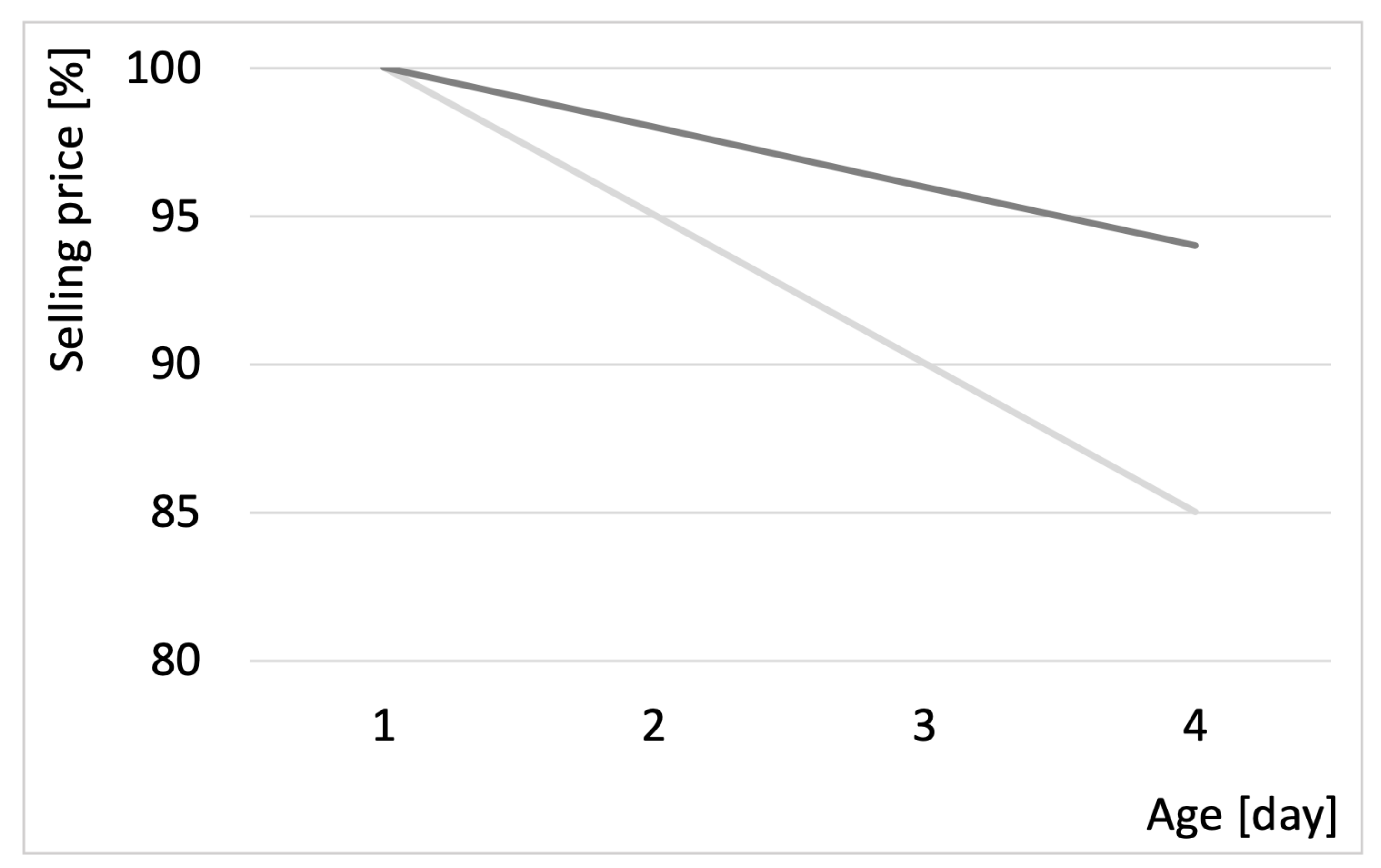
In order to address the problem under different realistic scenarios, we have generated 10 instances per company. In particular, we have generated the following data, by using a normal distribution with coefficient of variation equal to 0.10: ${\overline{Q}}_w$, $D_{tj}$, $G_t$$p_t^s$, $b_t^s$. The mean of the amount of weekly ripe product has been set to 60,000 kg and 22,000 kg, respectively, for $C_1$ and $C_2$. The mean of the daily demand from each DC has been set to 1600 kg and 600 kg, respectively, for the two suppliers, while about spot customers it has been set to 800 kg and 500 kg. The unit selling prices of the fresh product to the main customer has been estimated, from the historical data made available by the official website of the Italian Institute of Services for the Agricultural Food Market [43]. $b_t^s$ has been estimated assuming a 10% increase in the price to the main customer. The perishable nature of the agricultural products of the case study has been taken into consideration assuming a dependence of the market price on the age of the product, as shown in Figure 1. The two lines represent in what percentage the market value of the product decreases with increasing age: in the case of broccoli (i.e., light gray line), a decrease of 5% per day has been considered, while this value is 2% per day if we refer to artichokes (i.e., dark gray line).

In

Table 4. Case study: Relevant data.

	K	$\mathit{\tau }$	${\mathit{I}}_{max}$	$\mathit{\rho }$	$\mathit{\eta }$	$\mathit{\alpha }$	$\mathit{\lambda }$	$\mathit{\delta }$	$\mathit{\theta }$	h
	[unit]	[Day]	[kg]	[EUR/kg]	[EUR/Day]	[EUR/Kilometer]	[EUR/Minute]		[Hour]	[EUR/Kg]
$C_1$	2	4	30,000	0.10	800	0.30	0.15	0.85	-	0.03
$C_2$	1	4	10,000	0.15	500	0.30	0.15	-	10	0.10

, we show the remaining relevant data, retrieved from the current operating conditions of the two companies. A hyphen means that there is no unique value for the data, then it can be varied.

In

Table 5. Spatial distance between nodes [kilometer], referring to the first supplier.

	${\mathit{C}}_1$	${\mathit{DC}}_1$	${\mathit{DC}}_2$	${\mathit{DC}}_3$	${\mathit{DC}}_4$	${\mathit{DC}}_5$
$C_1$	0	392	433	55	277	619
$D{C}_1$	392	0	152	367	696	236
$D{C}_2$	433	152	0	405	583	337
$D{C}_3$	55	367	405	0	362	592
$D{C}_4$	277	696	583	362	0	851
$D{C}_5$	619	236	337	592	851	0

,

Table 6. Temporal distance between nodes [minute], referring to the first supplier.

	${\mathit{C}}_1$	${\mathit{DC}}_1$	${\mathit{DC}}_2$	${\mathit{DC}}_3$	${\mathit{DC}}_4$	${\mathit{DC}}_5$
$C_1$	0	235	276	51	188	360
$D{C}_1$	235	0	113	222	406	152
$D{C}_2$	276	113	0	245	343	215
$D{C}_3$	51	222	245	0	226	344
$D{C}_4$	188	406	343	226	0	480
$D{C}_5$	360	152	215	344	480	0

,

Table 7. Spatial distance between nodes [kilometer], referring to the second supplier.

	${\mathit{C}}_2$	${\mathit{DC}}_1$	${\mathit{DC}}_2$	${\mathit{DC}}_3$	${\mathit{DC}}_4$
$C_2$	0	512	739	604	691
$D{C}_1$	512	0	236	103	272
$D{C}_2$	739	236	0	145	161
$D{C}_3$	604	103	145	0	182
$D{C}_4$	691	272	161	182	0

and

Table 8. Temporal distance between nodes [minute], referring to the second supplier.

	${\mathit{C}}_2$	${\mathit{DC}}_1$	${\mathit{DC}}_2$	${\mathit{DC}}_3$	${\mathit{DC}}_4$
$C_2$	0	295	432	369	422
$D{C}_1$	295	0	144	73	171
$D{C}_2$	432	144	0	98	113
$D{C}_3$	369	73	98	0	124
$D{C}_4$	422	171	113	124	0

, the spatial and temporal distance between nodes for the case of first and second supplier are, respectively, shown. They have been recovered from GoogleMaps, taking into account the shortest path between each pair of nodes and the traffic conditions which occur in the part of the day in which the shipment usually takes place.

The computational experiments have been carried out on a PC running Windows 10 Pro with AMD Ryzen 7 2700X Eight-Core Processor 4.00 GHz/16 GB. The proposed optimization model has been solved by CPLEX 12.7, Academic License.

4.2. Computational Experiments and Managerial Insights—Tactical Level

4.2.1. Single-Supplier Model

At the tactical level, we have adopted $M_{SS}$, with the aim to determine the most profitable combination of two important parameters: the harvesting frequency (i.e., number of harvesting days per week) and the quality of service guaranteed to the DCs.

The choice of $\gamma$ is quite critical in that, harvesting very frequently corresponds to increase the costs related to the renting of the specialized harvesting equipment, but it allows to ship fresh products quite often; on the other hand, harvesting only in a few days of the week entails greater use of the warehouse to stock up and delivery of products with an average higher age (i.e., lower market value). Six alternatives have been explored, namely $\gamma \in \{2,\dots ,7\}$. Observe that $\gamma =1$ is not feasible because $\tau =4$ is not enough to ensure that DCs demand can be met every day.

Moreover, we have determined the service level, which maximizes the profit. In this case, $\theta \in \{9,10,11\}$ and $\delta \in \{0.75,0.85\}$ have been explored for the two companies, respectively. Observe that the values to be contractually guaranteed are, respectively, $\theta =11$ h and $\delta =0.75$, but some rewards are ensured in order to encourage the decrease of $\theta$ and the increase of $\delta$.

In

Table 9. Average KPIs for the case of $\theta =9$ h (company $C_1$).

KPI	$\mathit{\gamma }$
	2	3	4	5	6	7
Revenue Main [EUR]	119,336.37	123,304.78	124,484.04	125,568.56	125,946.92	125,724.96
Reward Main [EUR]	3282.25	3287.55	3274.44	3277.89	3270.17	3252.99
Revenue Spot [EUR]	11,920.63	12,287.85	13,014.80	12,961.07	13,369.76	14,153.24
Inventory Cost [EUR]	13,585.96	7049.99	4152.71	2550.25	1360.49	678.69
Fuel Cost [EUR]	22,897.35	22,894.17	22,894.26	22,894.17	22,894.26	22,894.17
Driver Cost [EUR]	7172.04	7170.87	7171.14	7170.87	7171.14	7170.87
Production Cost [EUR]	36,341.34	36,341.34	36,341.34	36,341.34	36,341.34	36,341.34
Havesting Cost [EUR]	9600.00	14,400.00	19,200.00	24,000.00	28,800.00	33,600.00
Number of trips [unit]	75.10	75.10	75.10	75.10	75.10	75.10
Average product age [day]	2.18	1.62	1.37	1.22	1.10	1.02
Profit [EUR]	44,942.56	51,023.81	51,013.84	48,850.89	46,019.62	42,446.12

,

Table 10. Average KPIs for the case of $\theta =10$ h (company $C_1$).

KPI	$\mathit{\gamma }$
	2	3	4	5	6	7
Revenue Main [EUR]	119,280.69	123,288.01	124,382.05	125,457.42	125,893.95	125,725.60
Reward Main [EUR]	1640.31	1643.21	1635.84	1637.65	1634.26	1626.49
Revenue Spot [EUR]	11,976.92	12,331.40	13,127.04	13,072.11	13,436.19	14,153.24
Inventory Cost [EUR]	13,594.38	7093.31	4171.01	2556.52	1380.45	680.04
Fuel Cost [EUR]	20,513.85	20,507.28	20,517.18	20,507.22	20,509.71	20,509.71
Driver Cost [EUR]	6520.79	6517.62	6521.78	6517.58	6518.81	6518.81
Production Cost [EUR]	36,341.34	36,341.34	36,341.34	36,341.34	36,341.34	36,341.34
Harvesting Cost [EUR]	9600.00	14,400.00	19,200.00	24,000.00	28,800.00	33,600.00
Number of trips [unit]	72.00	71.80	72.00	71.80	71.90	71.90
Average product age [day]	2.19	1.62	1.37	1.22	1.10	1.02
Profit [EUR]	46,327.57	52,403.08	52,393.63	50,244.52	47,414.10	43,855.43

and

Table 11. Average KPIs for the case of $\theta =11$ h (company $C_1$).

KPI	$\mathit{\gamma }$
	2	3	4	5	6	7
Revenue Main [EUR]	119,277.87	123,239.61	124,400.55	125,402.91	125,905.51	125,729.52
Reward Main [EUR]	0.00	0.00	0.00	0.00	0.00	0.00
Revenue Spot [EUR]	11,979.01	12,351.49	13,098.85	13,136.66	13,412.93	14,153.24
Inventory Cost [EUR]	13,587.89	7056.84	4159.49	2561.87	1363.99	686.19
Fuel Cost [EUR]	20,210.28	20,194.41	20,196.75	20,194.35	20,196.30	20,195.55
Driver Cost [EUR]	6429.46	6425.54	6425.69	6424.73	6426.14	6425.03
Production Cost [EUR]	36,341.34	36,341.34	36,341.34	36,341.34	36,341.34	36,341.34
Harvesting Cost [EUR]	9600.00	14,400.00	19,200.00	24,000.00	28,800.00	33,600.00
Number of trips [unit]	68.50	68.40	68.40	68.30	68.40	68.30
Average product age [day]	2.19	1.62	1.37	1.22	1.10	1.02
Profit [EUR]	45,087.91	51,172.98	51,176.14	49,017.28	46,190.68	42,634.65

, we report the computational results of the experiments carried out on the 10 instances generated with reference to the first supplier. We highlight the average value of 10 key performance indicators (KPIs). The first eight KPIs characterize the objective funcion (2) of $M_{SS}$. Moreover, we show the number of trips and the average age of the product shipped to the main customer and spot customers. First of all, we can say that the average profit, fixed $\theta$, initially increases as the harvesting frequency increases until it reaches the peak when $\gamma \in \{3,4\}$. Then, it starts to significantly decrease. The reasons behind this trend are multiple. As it can be noted, the increase in the harvesting frequency has two main effects: the revenue (main and spot) increases because the average age of the product delivered decreases, while storage costs decrease significantly. These two benefits are “paid” through the increase in harvesting costs. When $\gamma \in \{5,6,7\}$, the benefits obtained can no longer offset the additional costs of the harvesting, therefore the average profit significantly reduces. Note that the routing costs remain constant because all the parameters related to the distribution activities remain unchanged. Next, we analyze how KPIs change, by fixing $\gamma$ and varying $\theta$. Here, we have two main contrasting effects: the reward insured by the main customer, and the routing costs. The reward pushes towards a reduction of the daily time limit, but this entails a significant increase in the routing costs because the flexibility in the choice of the routes is reduced (observe that, as expected, the number of trips reduces as $\theta$ increases). Basically, we can say that when $\theta =10$ h, the additional revenue from the main customer is enough to cover the increase in routing costs and to guarantee the best profitability. At the tactical level, the use of $M_{SS}$ referring to $S_1$, suggests the following setting: $\gamma =3$ and $\theta =10$. Observe that, when $\gamma \in \{3,4\}$ the average profit is very similar. However, when the harvesting frequency is three days per week, the average quality of the product shipped is higher, and this aspect could favor customer’s satisfaction and loyalty in the mid term.

In

Table 12. Average KPIs for the case of $\delta =0.75$ (company $C_2$).

KPI	$\mathit{\gamma }$
	2	3	4	5	6	7
Revenue Main [EUR]	78,878.70	79,015.54	79,048.03	78,371.14	76,767.99	76,219.58
Reward Main [EUR]	0.00	0.00	0.00	0.00	0.00	0.00
Revenue Spot [EUR]	14,363.05	15,320.20	15,604.37	16,385.33	17,908.06	18,301.31
Inventory Cost [EUR]	11,245.55	6088.99	3883.02	2462.91	1329.36	798.99
Fuel Cost [EUR]	19,081.74	19,081.74	19,081.74	19,081.74	19,081.74	19,081.74
Driver Cost [EUR]	5835.63	5835.63	5835.63	5835.63	5835.63	5835.63
Production Cost [EUR]	10,193.62	10,193.62	10,193.62	10,193.62	10,193.62	10,193.62
Harvesting Cost [EUR]	7200.00	10,800.00	14,400.00	18,000.00	21,600.00	25,200.00
Number of trips [unit]	41.70	41.70	41.70	41.70	41.70	41.70
Average product age [day]	2.02	1.56	1.35	1.23	1.13	1.08
Profit [EUR]	39,685.21	42,335.75	41,258.39	39,182.57	36,635.70	33,410.91

and

Table 13. Average KPIs for the case of $\delta =0.85$ (company $C_2$).

KPI	$\mathit{\gamma }$
	2	3	4	5	6	7
Revenue Main [EUR]	81,140.74	81,611.02	81,650.38	80,820.37	79,846.40	79,279.38
Reward Main [EUR]	1368.48	1361.19	1353.85	1338.96	1325.22	1315.94
Revenue Spot [EUR]	11,439.08	12,254.63	12,570.39	13,562.64	14,414.08	14,699.79
Inventory Cost [EUR]	11,624.28	6360.80	4048.40	2588.84	1385.03	719.20
Fuel Cost [EUR]	19,081.74	19,081.74	19,081.74	19,081.74	19,084.14	19,081.74
Driver Cost [EUR]	5835.63	5835.63	5835.63	5835.63	5836.43	5835.63
Production Cost [EUR]	10,193.62	10,193.62	10,193.62	10,193.62	10,193.62	10,193.62
Harvesting Cost [EUR]	7200.00	10,800.00	14,400.00	18,000.00	21,600.00	25,200.00
Number of trips [unit]	41.70	41.70	41.70	41.70	41.70	41.70
Average product age [day]	2.05	1.57	1.36	1.23	1.13	1.08
Profit [EUR]	40,013.02	42,955.04	42,015.23	40,022.14	37,486.49	34,264.93

, the computational results of the experiments conducted on the 10 instances related to $C_2$ are shown. When the service level is fixed, the profit varies by varying $\gamma$. As the harvesting frequency increases, most of the shipments concern the fresh product, therefore the storage costs decrease drastically. The overall revenue increases because the product delivered is on average “younger” and then better paid. In particular, profit is maximized when $\gamma =3$. If the service level is varied, a reward must be taken into account when $\delta =0.85$. In this case, the larger amount of product to be guaranteed daily to the main customer implies the loss of some market opportunities offered by spot customers. However, the revenue increase from the main customer is higher than the revenue decrease from spot customers, therefore this solution is more convenient, whatever the harvesting frequency. It should be noted that in any case the routing costs do not vary, as parameters related to distribution remain unchanged. Basically, with reference to the second supplier, our optimization model $M_{SS}$ suggests the setting $\gamma =3$ and $\delta =0.85$.

4.2.2. Collaboration between Suppliers

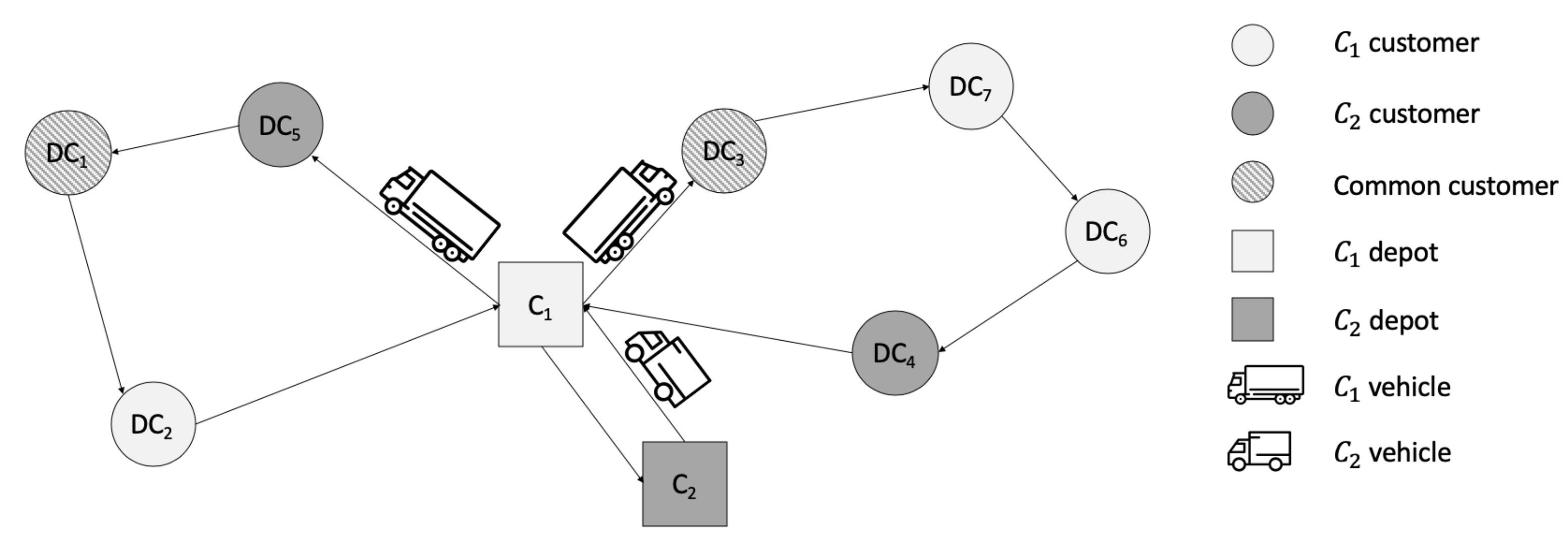
Since suppliers $C_1$ and $C_2$ are geographically very close and share two customers, at the tactical level we have also explored the possibility of collaboration in the distribution of goods. In particular, we have solved $M_{CR}$, using as input the output of $M_{SS}$ in terms of amount to be shipped to each DC by each supplier at each period. This means that the decisions about harvesting and storage are fixed, while new solutions are possibile for the routing phase. Figure 2 shows a graphical example of horizontal collaboration between the two suppliers. Basically, $C_2$ sends its goods to $C_1$ incurring a routing cost for the round trip from its depot to that of the other supplier, which acts as a hub. At the hub, the goods are transferred from the $C_2$ vehicle to the $C_1$ fleet, which deals with the delivery of the agri-products to the DCs in exchange for a fee.

We have solved $M_{CR}$ on ten datasets, obtained by randomly combining the ten instances generated for the two companies, and under the most profitable parameter setting, according to the discussion made in the previous subsection. The only exception was that, the time limit was fixed to 11 h for the DCs of $C_1$, which are not shared with $C_2$, in order to guarantee the feasibility of the problem. We have supposed to implement the horizontal collaboration in any period of the time horizon. The mean computational time was around 15 s.

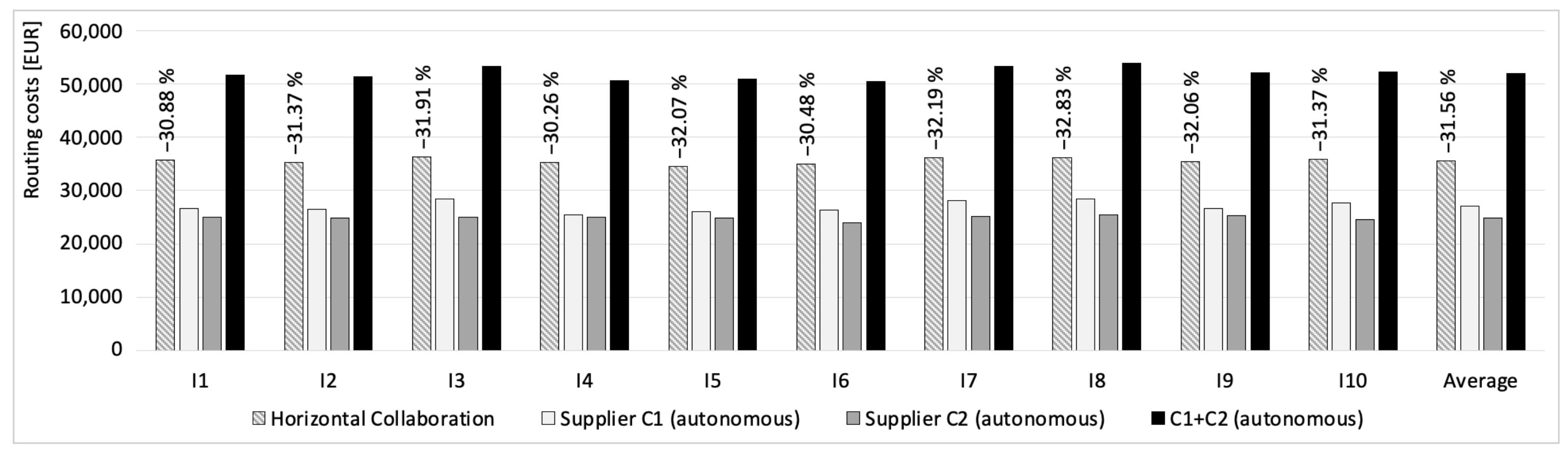
In Figure 3, we show how the routing costs vary in the two cases of autonomous and collaborative distribution.

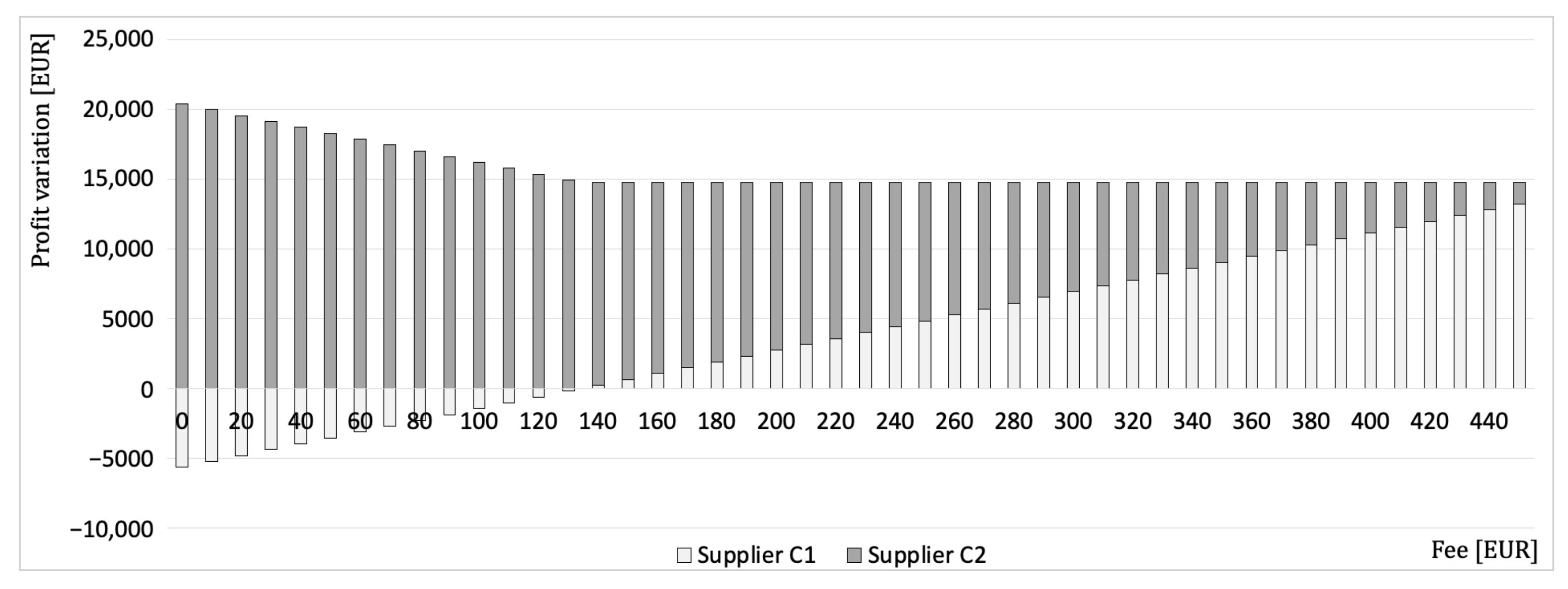
As it can be noted, the implementation of the collaborative routing leads to an average reduction in fuel and driver costs of 31.56%, which corresponds to about 16,400 EUR. However, an important issue concerns the percentage of sharing of such saving between the two suppliers, which mainly depends on the amount of the fee that $C_2$ pays to $C_1$ for having the service. In Figure 4, we represent how the profit varies between the two suppliers, as the fee varies. If the service was performed free of charge by supplier $C_1$, this latter would incur a loss of approximately 5600 EUR compared to non-collaboration, caused by the additional routing costs and the lack of reward from the main customer. Instead, $C_2$ would have to bear the only costs to move to and from the $C_1$ depot, therefore it would have a total saving of about 20,000 EUR. Looking at the graph, we can say that a fee of at least 140 EUR/day is required for supplier $C_1$ to make profitable the collaboration with $C_2$. However, the amount of fee which makes collaboration, convenient in the same way for the two suppliers, is about 310 EUR/day because the average profit increase is distributed in the fairest way.

4.3. Computational Experiments and Managerial Insights—Operational Level

At the operational level, the two companies must make 4 types of decisions, which are listed below:

• harvesting decisions: if and how much to harvest;
• inventory decisions: amount of product of each age to store;
• shipping decisions: amount of product of each age to ship to the main customer and spot customers;
• routing decisions: routes to reach the different DCs.

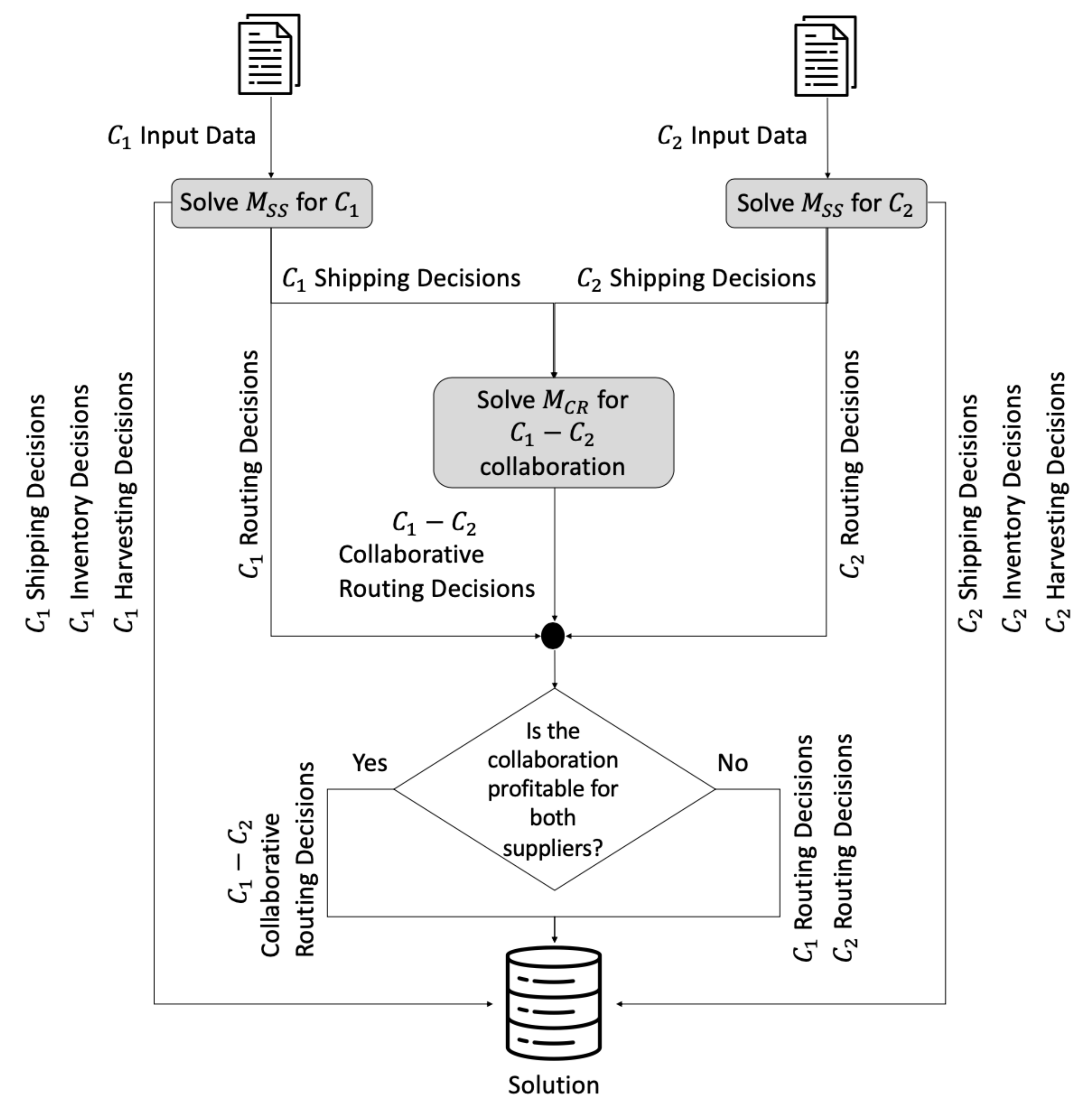
With the aim to support the two suppliers operationally, we have proposed a framework, which is schematized in Figure 5.

It suggests the best decisions to maximize the overall profit and verifies if horizontal collaboration is convenient or not, once a daily fee $\omega$ has been fixed.

Given a well defined time horizon, the first step is to solve Model $M_{SS}$ separately for the two suppliers. The harvesting, inventory and shipping decisions, output of $M_{SS}$ are inserted into the solution of the overall problem.

At the second step, Model $M_{CR}$ is solved. It receives the shipping decisions as input and returns the collaborative routes and their relative cost.

At the third step, the profitability of the collaboration for both suppliers is checked. If yes, the routing decisions resulting from the $M_{CR}$ model are inserted into the solution. Otherwise, the collaboration is not implemented and autonomous routing decisions, output of the respective models $M_{SS}$, are inserted into the overall solution.

We have solved separately $M_{SS}$ for $C_1$ and $C_2$, on the ten instances generated for each company, and considering only one week as time horizon. Then, we have solved $M_{CR}$ on the ten datasets, obtained by randomly combining the ten instances generated for each company. We have considered the three different scenarios in

Table 14. The three different scenarios for the operational level.

Scenario	$\mathit{\omega }$ [EUR/Day]
$Sc1$—$C_1$ has less bargaining power than $C_2$	100.00
$Sc2$—$C_1$ has greater bargaining power than $C_2$	500.00
$Sc3$—$C_1$ and $C_2$ have the same bargaining power	310.00

, in terms of fee that $C_2$ pays to $C_1$ for having the distribution service. The computational time was not longer than 2 min in all cases.

In

Table 15. Profit comparison mous and collaborative distribution under the three different scenarios.

	Profit [EUR]		Profit Increase [%]
	Autonomy		Collaboration—$Sc1$			Collaboration—$Sc2$			Collaboration—$Sc3$
	$C_1$	$C_2$	$C_1$	$C_2$	Total	$C_1$	$C_2$	Total	$C_1$	$C_2$	Total
I1	7142.65	7414.50	1.04	8.19	4.68	16.25	0.86	8.41	13.03	15.04	14.06
I2	5332.24	1314.29	3.45	100.69	22.68	12.57	3.77	10.83	25.05	78.00	35.52
I3	9363.34	3591.73	1.65	55.66	16.62	13.46	1.58	10.17	16.14	35.70	21.56
I4	9589.83	4583.81	0.78	27.52	9.43	18.45	2.49	13.29	11.09	25.74	15.83
I5	10,656.61	7734.92	1.13	19.41	8.82	2.80	0.34	1.76	12.13	15.09	13.38
I6	6679.89	1981.08	1.00	37.98	9.46	9.36	2.27	7.74	13.48	52.40	22.38
I7	12,762.68	577.99	0.73	203.52	9.51	6.72	8.57	6.80	10.36	217.77	19.35
I8	4235.38	4508.95	5.08	64.68	35.82	61.68	3.11	31.48	39.79	32.08	35.82
I9	15,232.41	3969.68	0.57	36.00	7.89	9.50	2.00	7.95	9.16	30.82	13.64
I10	10,251.36	4542.15	0.67	17.45	5.82	7.97	1.67	6.03	8.01	23.91	12.89
Avg	9124.64	4021.91	1.25	34.21	11.33	12.62	1.74	9.29	13.43	29.40	18.32

, we show the results of our computational experience at the operational level. The profit in case of autonomous distribution is compared with the three scenarios of collaborative distribution. As expected, the collaboration brings benefits for both suppliers according to all 3 scenarios. The first two scenarios favor the second and the first supplier, respectively. While the third scenario allows the maximization of the benefits for both the companies, with an average increase in overall profit of 18.32%. Observe that under the third scenario, collaboration is implemented on average in 94% of the days, which means that it is almost always profitable for both companies. This percentage drops to 51% and 44%, respectively, if we refer to the first two scenarios.

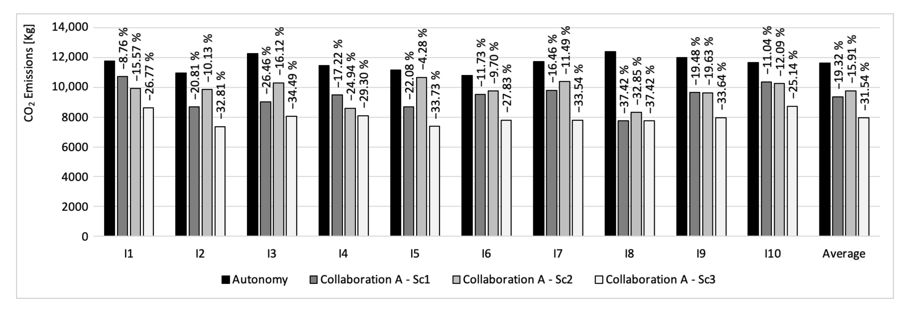
Next, we briefly report the benefits that collaboration can bring to the environment. We refer to carbon dioxide (CO${}_2$) emissions, whose conversion factor is estimated at 2.63 kg/L, as in [38]. In Figure 6, the amount of CO${}_2$ emissions (kg) in the case of absence of collaboration between the two suppliers is compared with the 3 collaborative scenarios. Basically, the collaboration leads to a significant reduction in CO${}_2$ emissions in all cases. In particular, in the third scenario there is an average reduction of over 31%, which is one more reason to prefer collaborative routing.

5. Conclusions

In this paper, we have proposed two optimization models to support the decision-making of two agri-companies, which deal with perishable products. Their business concerns planting, growing, harvesting, inventory, and delivery management of fresh vegetables. They have a main contract customer, who has a set of DCs to be daily served, but they can also exploit the opportunities offered by a spot market. The first model aims to maximize profit of a single agri-company and concerns the integration and coordination of the harvesting, storage, delivery and routing decisions. Through a computational experience conducted on a set of real-life instances, it was possible to identify the most profitable parameter setting, in terms of the optimal number of days of the week to be dedicated to harvesting activities and the quality of service to be guaranteed to the customers. In particular, for the first company it was suggested to serve all the DCs relating to the main customer within a time limit of 10 h, while for the second to satisfy at least 85% of the main customer’s demand. In both cases, the optimal number of harvesting days per week was found to be equal to 3. The second model instead allowed to explore and assess the benefits achievable from the horizontal collaboration between the two companies of the case study for what concerns the distribution activities. Computational experience has revealed that an overall saving on routing costs of up to 31–32% is achievable. At the operational level, a heuristic framework was presented and implemented in order to jointly support the two companies on a daily basis. The results showed that horizontal collaboration can lead to an average increase in profit of up to 18.32% and a reduction in CO${}_2$ emissions of up to 31.54%, when the two companies have similar bargaining power. Overall, horizontal collaboration represents an extremely useful and valuable solution, which can be applied in multiple situations and allows for an improvement in company economic parameters.

Future developments concern a multi-product and multi-company version of the first of the two optimization models introduced.

References

- Cox, B.D.; Wichelow, M.J.; Prevost, T. Seasonal consumption of salad vegetables and fresh fruit in relation to the development of cardiovascular disease and cancer. Public Health Nutr. 2000, 3, 19–29. [Google Scholar] [CrossRef] [PubMed] [Green Version]
- Wang, P.-Y.; Fang, J.-C.; Gao, Z.-H.; Zhang, C.; Xie, S.-Y. Higher intake of fruits, vegetables or their fiber reduces the risk of type 2 diabetes: A meta-analysis. J. Diabetes Investig. 2015, 7, 56–69. [Google Scholar] [CrossRef]
- Villalobos, J.R.; Soto-Silva, W.E.; Gonzalez-Araya, M.C.; Gonzalez-Ramirez, R.G. Research directions in technology development to support real-time decisions of fresh produce logistics: A review and research agenda. Comput. Electron. Agric. 2019, 167, 105092. [Google Scholar] [CrossRef]
- Guido, R.; Mirabelli, G.; Palermo, E.; Solina, V. A framework for food traceability: Case study – Italian extra-virgin olive oil supply chain. Int. J. Ind. Eng. Manag. 2020, 11, 50–60. [Google Scholar] [CrossRef]
- Fahimnia, B.; Farahani, R.Z.; Marian, R.; Luong, L. A review and critique on integrated production–distribution planning models and techniques. J. Manuf. Syst. 2013, 32, 1–19. [Google Scholar] [CrossRef]
- Li, Y.; Chu, F.; Coté, J.F.; Coelho, L.C.; Chu, C. The multi-plant perishable food production routing with packaging consideration. Int. J. Prod. Econ. 2020, 221, 107472. [Google Scholar] [CrossRef]
- Neves-Moreira, F.; Almada-Lobo, B.; Cordeau, J.F.; Guimares, L.; Jans, R. Solving a large multi-product production-routing problem with delivery time windows. Omega 2019, 86, 154–172. [Google Scholar] [CrossRef]
- Chandra, P.; Fisher, M.L. Coordination of production and distribution planning. Eur. J. Oper. Res. 1994, 72, 503–517. [Google Scholar] [CrossRef]
- Vahdani, B.; Niaki, S.T.A.; Aslanzade, S. Production-inventory-routing coordination with capacity and time window constraints for perishable products: Heuristic and metaheuristic algorithms. J. Clean. Prod. 2017, 161, 598–618. [Google Scholar] [CrossRef]
- Amorim, P.; Gunther, H.-O.; Almada-Lobo, B. Multi-objective integrated production and distribution planning of perishable products. Int. J. Prod. Econ. 2012, 138, 89–101. [Google Scholar] [CrossRef]
- Al Shamsi, A.; Al Raisi, A.; Aftab, M. Pollution-Inventory Routing Problem with Perishable Goods. In Logistics Operations, Supply Chain Management and Sustainability; Springer: Cham, Switzerland, 2014; pp. 585–596. [Google Scholar]
- De Moraes, C.C.; de Oliveira Costa, F.H.; Pereira, C.R.; da Silva, A.L.; Delai, I. Retail food waste: Mapping causes and reduction practices. J. Clean. Prod. 2020, 256, 120124. [Google Scholar] [CrossRef]
- De Steur, H.; Wesana, J.; Dora, M.K.; Pearce, D.; Gellynck, X. Applying Value Stream Mapping to reduce food losses and wastes in supply chains: A systematic review. Waste Manag. 2016, 58, 359–368. [Google Scholar] [CrossRef] [Green Version]
- Papargyropoulou, E.; Lozano, R.; Steinberger, J.K.; Wright, N.; Ujang, Z.B. The food waste hierarchy as a framework for the management of food surplus and food waste. J. Clean. Prod. 2014, 76, 106–115. [Google Scholar] [CrossRef]
- Fredriksson, A.; Liljestrand, K. Capturing food logistics: A literature review and research agenda. Int. J. Logist. Res. Appl. 2015, 19, 16–34. [Google Scholar] [CrossRef]
- Amorim, P.; Meyr, H.; Almeder, C.; Almada-Lobo, B. Managing perishability in production-distribution planning: A discussion and review. Flex. Serv. Manuf. J. 2013, 25, 389–413. [Google Scholar] [CrossRef]
- Chen, H.-K.; Hsueh, C.-F.; Chang, M.-S. Production scheduling and vehicle routing with time windows for perishable food products. Comput. Oper. Res. 2009, 36, 2311–2319. [Google Scholar] [CrossRef]
- Bustos, C.A.; Moors, E.H.M. Reducing post-harvest food losses through innovative collaboration: Insights from the Colombian and Mexican avocado supply chains. J. Clean. Prod. 2018, 199, 1020–1034. [Google Scholar] [CrossRef] [Green Version]
- Nahmias, S. Perishable Inventory Theory: A Review. Oper. Res. 1982, 30, 680–708. [Google Scholar] [CrossRef]
- Coelho, L.C.; Laporte, G. Optimal joint replenishment, delivery and inventory management policies for perishable products. Comput. Oper. Res. 2014, 47, 42–52. [Google Scholar] [CrossRef]
- Hsiao, H.-I.; Tu, M.; Yang, M.-F.; Tseng, W.-C. Deteriorating inventory model for ready-to-eat food under fuzzy environment. Int. J. Logist. Res. Appl. 2017, 20, 560–580. [Google Scholar] [CrossRef]
- Huang, H.; He, Y.; Li, D. Pricing and inventory decisions in the food supply chain with production disruption and controllable deterioration. J. Clean. Prod. 2018, 180, 280–296. [Google Scholar] [CrossRef]
- Diaz-Madronero, M.; Peidro, D.; Mula, J. A review of tactical optimization models for integrated production and transport routing planning decisions. Comput. Ind. Eng. 2015, 88, 518–535. [Google Scholar] [CrossRef]
- Adulyasak, Y.; Cordeau, J.F.; Jans, R. The production routing problem: A review of formulations and solution algorithms. Comput. Oper. Res. 2015, 55, 141–152. [Google Scholar] [CrossRef]
- Rong, A.; Akkermn, R.; Grunow, M. An optimization approach for managing fresh food quality throughout the supply chain. Int. J. Prod. Econ. 2011, 131, 421–429. [Google Scholar] [CrossRef]
- Jia, T.; Li, X.; Wang, N.; Li, R. Integrated Inventory Routing Problem with Quality Time Windows and Loading Cost for Deteriorating Items under Discrete Time. Math. Probl. Eng. 2014, 2014, 1–14. [Google Scholar] [CrossRef]
- Seyedhosseini, S.M.; Ghoreyshi, S.M. An integrated model for production and distribution planning of perishable products with inventory and routing considerations. Math. Probl. Eng. 2014, 2014, 1–10. [Google Scholar] [CrossRef] [PubMed]
- Li, Y.; Chu, F.; Yang, Z.; Calvo, R.W. A Production Inventory Routing Planning for Perishable Food with Quality Consideration. IFAC-PapersOnLine 2016, 49, 407–412. [Google Scholar] [CrossRef]
- Ghasemkhani, A.; Tavakkoli-Moghaddam, R.; Shahnejat-Bushehri, S.; Momen, S.; Tavakkoli-Moghaddam, H. An integrated production inventory routing problem for multi perishable products with fuzzy demands and time windows. IFAC-PapersOnLine 2019, 52, 523–528. [Google Scholar] [CrossRef]
- Qiu, Y.; Qiao, J.; Pardalos, P.M. Optimal production, replenishment, delivery, routing and inventory management policies for products with perishable inventory. Omega 2019, 82, 193–204. [Google Scholar] [CrossRef]
- Li, Y.; Chu, F.; Feng, C.; Chu, C.; Zhou, M. Integrated Production Inventory Routing Planning for Intelligent Food Logistics Systems. IEEE Trans. Intell. Transp. Syst. 2019, 20, 867–878. [Google Scholar] [CrossRef]
- Chan, F.T.S.; Wang, Z.X.; Goswami, A.; Singhania, A.; Tiwari, M.K. Multi-objective particle swarm optimization based integrated production inventory routing planning for efficient perishable food logistics operations. Int. J. Prod. Res. 2020, 58, 5155–5174. [Google Scholar] [CrossRef]
- Manouchehri, F.; Nookabadi, A.S.; Kadivar, M. Production routing in perishable and quality degradable supply chains. Heliyon 2020, 6, 2. [Google Scholar] [CrossRef] [PubMed]
- Gansterer, M.; Hartl, R.F. Collaborative vehicle routing: A survey. Eur. J. Oper. Res. 2018, 268, 1–12. [Google Scholar] [CrossRef] [Green Version]
- Son, J.Y.; Ghosh, S. Vendor managed inventory with fixed shipping cost allocation. Int. J. Logist. Res. Appl. 2020, 23, 1–23. [Google Scholar] [CrossRef]
- Vlachos, I.P.; Bourlakis, M.; Karalis, V. Manufacturer–retailer collaboration in the supply chain: Empirical evidence from the Greek food sector. Int. J. Logist. Res. Appl. 2008, 11, 267–277. [Google Scholar] [CrossRef]
- Treitl, S.; Nolz, P.C.; Jammernegg, W. Incorporating environmental aspects in an inventory routing problem. A case study from the petrochemical industry. Flex. Serv. Manuf. J. 2014, 26, 143–169. [Google Scholar] [CrossRef]
- Soysal, M.; Bloemhof-Ruwaard, J.M.; Haijema, R.; van der Vorst, J.G.A.J. Modeling a green inventory routing problem for perishable products with horizontal collaboration. Comput. Oper. Res. 2018, 89, 168–182. [Google Scholar] [CrossRef]
- Badraoui, I.; Van der Vorst, J.G.A.J.; Boulaksil, Y. Horizontal logistics collaboration: An exploratory study in Morocco’s agri-food supply chains. Int. J. Logist. Res. Appl. 2020, 23, 85–102. [Google Scholar] [CrossRef] [Green Version]
- Fernandez, E.; Fontana, D.; Speranza, M.G. On the Collaboration Uncapacitated Arc Routing Problem. Comput. Oper. Res. 2016, 67, 120–131. [Google Scholar] [CrossRef] [Green Version]
- Gaudioso, M.; Giallombardo, G.; Miglionico, G. A savings-based model for two-shipper cooperative routing. Optim. Lett. 2018, 12, 1811–1824. [Google Scholar] [CrossRef]
- Krajewska, M.A.; Kopfer, H.; Laporte, G.; Ropke, S.; Zaccour, G. Horizontal cooperation among freight carriers: Request allocation and profit sharing. J. Oper. Res. Soc. 2008, 59, 1483–1491. [Google Scholar] [CrossRef]
- Italian Institute of Services for the Agricultural Food Market. Available online: http://www.ismeamercati.it/analisi-e-studio-filiere-agroalimentari (accessed on 19 March 2021).
Figure 1.
Selling price variation of broccoli and artichokes according to age.
Figure 2.
Graphical example of horizontal collaboration between the two suppliers.
Figure 3.
Routing costs [EUR] in the cases of autonomous and collaborative distribution.
Figure 4.
Average profit variation for the two suppliers, by varying the fee.
Figure 5.
Framework for the operational level.
Figure 6.
Comparison in terms of CO emissions reduction between autonomous and collaborative distribution.