
De-Noising Process in Room Impulse Response with Generalized Spectral Subtraction


Department of Mechanical and Automotive Engineering, University of Ulsan, 93 Daehak-ro, Nam-Gu, Ulsan 44610, Korea
*
Author to whom correspondence should be addressed.
Appl. Sci. 2021, 11(15), 6858; https://0-doi-org.brum.beds.ac.uk/10.3390/app11156858
Submission received: 1 July 2021
/
Revised: 23 July 2021
/
Accepted: 23 July 2021
/
Published: 26 July 2021
(This article belongs to the Section Acoustics and Vibrations)
Abstract
:The generalized spectral subtraction algorithm (GBSS), which has extraordinary ability in background noise reduction, is historically one of the first approaches used for speech enhancement and dereverberation. However, the algorithm has not been applied to de-noise the room impulse response (RIR) to extend the reverberation decay range. The application of the GBSS algorithm in this study is stated as an optimization problem, that is, subtracting the noise level from the RIR while maintaining the signal quality. The optimization process conducted in the measurements of the RIRs with artificial noise and natural ambient noise aims to determine the optimal sets of factors to achieve the best noise reduction results regarding the largest dynamic range improvement. The optimal factors are set variables determined by the estimated SNRs of the RIRs filtered in the octave band. The acoustic parameters, the reverberation time (RT), and early decay time (EDT), and the dynamic range improvement of the energy decay curve were used as control measures and evaluation criteria to ensure the reliability of the algorithm. The de-noising results were compared with noise compensation methods. With the achieved optimal factors, the GBSS contributes to a significant effect in terms of dynamic range improvement and decreases the estimation errors in the RTs caused by noise levels.
1. Introduction
Reverberation time (RT) is the most representative and physically important parameter related to the average properties of a room [1,2,3] and is essential for predicting speech intelligibility [4,5]. A well-known and widely used method to calculate RT is determined by the energy decay curve (EDC) generated by Schroeder’s method [6]; however, the measured room impulse response (RIR) presents ambient noise, and equipment noise may deteriorate the EDC, leading to errors in predicting room acoustic parameters [7,8]. The relative errors for RTs, early decay time (EDT), and other acoustic parameters, without noise compensation, could exceed 5% [9,10].
In the past few decades, studies and achievements have been based on using mathematical models to improve the accuracy of estimating RT, etc. To minimize the noise effects in the backward integration method, typical research focused on the noise compensation method to truncate the RIR at a point where the RIR decay intersects with the constant noise floor [7], which is technically the truncation time, to generate noise-free decay curves [11,12]. Nevertheless, the performance of EDCs generated from different compensation methods is significantly influenced by the estimated upper integration time and the noise levels at the truncation time [13]. This problem identified two casual factors: the upper integration time of RIR and the estimated background noise levels at the truncation time. Consequently, a correction term was added to the integration to prevent the truncation error [9,13,14]. For mathematical advantages, nonlinear regression methods [15] were investigated to fit the RIR to calculate the slope of the EDC. The technique was further developed as an automated detection method for calculating the correction term and determining the truncation time [5,8]. All the methods were set out from the time domain. Advanced technical methods have been applied to remove the non-decaying frequency-dependent noise floor of the direction room impulse response, measured with spherical microphone arrays with an exponentially decaying zero-mean Gaussian noise [16,17]. An application of wavelet techniques for reducing the RT estimation error caused by noise showed the possibility of implementing the de-noising approach to reduce the noise of RIR [18].
Regarding well-known de-noising techniques involving a forward and an inverse Fourier transform [19] performed on the Frequency domain, spectral subtraction algorithms (SS) that have extraordinary ability in removing the signal noise levels were considered to minimize the noise effects on estimating acoustic parameters, such as RTs and EDT. The technique was used to de-noise the RIR because the algorithm has a similar de-noising rule to the noise subtraction method [20], in which the noise levels were subtracted from the noisy signal to estimate the clean signal. Unlike the SS algorithm, the de-noising processing of the noise subtraction method was conducted in the time domain. In contrast, the SS algorithms used a novel noise estimation approach to adaptively estimate the addictive noise levels during the silent periods of the signal and were subtracted from the noisy signals frame-by-frame. The methods were studied intensively based on short-time spectral amplitudes (STSA) and were used to suppress the noise with a relatively stable power spectral density. They were initially proposed for speech enhancement [21] and had been applied successfully in other areas, such as underwater acoustic sounds [22], speech dereverberation [23], and electronic noise reduction [24,25]. Nevertheless, the random variations of noise leading to an inaccurate estimation of the noise levels and the processing of noise subtraction may result in much of the interfering noise remaining, causing some original signals to be removed [26].
Many algorithms have been developed to minimize the distortion caused by noise subtraction processing between an enhanced signal and a clean signal [27]. Among these methods, Berouti proposed a generalized spectral subtraction based on short-time spectral amplitudes, called Berouti’s GSS (GBSS), which was implemented to de-noise the RIRs because of its computational simplicity and the flexibility of parametric adjustments in the technique for producing significant de-noising improvements [28,29,30,31,32,33,34]. The ultimate purpose of the algorithm was used to extend the reverberation decay range of the EDCs for RTs estimation. The corresponding two factors, an over subtraction factor and a spectral floor parameter, were used to maintain the trade-off between the remaining noise levels and the signal quality. However, subtracting a constant ratio of noise levels over the entire frequency of the RIR may also remove parts of the clean signal and deteriorate the estimation of the RTs. Therefore, it is essential to have prior knowledge of the motivation of the parameters of the GBSS algorithm to determine the optimal sets of factors to mitigate unwanted noise effects and improve the dynamic range, without or with an acceptable minimal degradation of the reverberation decay.
The subject of this paper is to investigate the possibilities of implementing the GBSS algorithm in de-noising the RIRs to extend the reverberation decay range of the corresponding EDCs. Because the algorithm is based on a hypothesis that the noise is relatively stable or a slowly varying process, the measurements are conducted in the “real-world” with a relative stable background noise. The most promising factors of the GBSS algorithm, including the over-subtraction factor and the spectral flooring factor, were used to suppress the noise levels. The optimal factors were achieved experimentally through measurements of the RIRs with artificial noise added and the natural ambient noise improve the dynamic range of the EDCs significantly, which is analyzed in detail in Section 4. In the de-noising processing, the parameters of RTs, EDT, and the dynamic range were used as the control measures and the evaluation criteria to ensure the accuracy of the RIR de-noising processing. The acoustic parameters estimated from the EDCs of the de-noised RIRs, with acceptable degradation of the reverberation decay rate, were compared to the compensation method. The proposed algorithm gave somewhat more stable results in some cases. Furthermore, the GBSS algorithm with optimal factors significantly improved the dynamic range and decreased the estimation errors in RTs caused by noise levels.
2. Principle of Spectral Subtraction
2.1. Basic Spectral Subtraction
The spectral subtraction algorithm is one of the earliest and longest-used techniques for background noise reduction and has been mainly applied to improve the quality of speech [21]. The basic principle is to subtract the magnitude spectrum of noise from the noisy signals where the signal and noise are considered uncorrelated. The method assumes that speech and noise are uncorrelated, and noise is added in the time domain, which is why the SS algorithm is applied to de-noise the RIRs, because the background noise presented in the RIRs is assumed to be additive noise. The discrete-time noisy RIR is composed of a clean signal, , and the noise is expressed as,
In the application of the SS, the discrete Fourier transform (DFT) of both sides is taken, where the general form of the enhanced signal spectrum can be described in terms of its magnitude spectrum of one frame, as follows,
where is the estimated noise spectrum and the updated during periods of silence and, is the enhanced signal spectrum calculated using the inverse Fourier transform with the information of phase of the original signal . When reconstructing the enhanced signal, its phase is approximated by the phase of the original signal, owing to the estimated phase of the noise spectrum, causing a sharp increase in the complexity of the algorithm, and when the SNR is comparatively high, leading to an imperceptible phase difference [29,30]. The value is the exponent determining the transition sharpness, = 2 represents the power spectral subtraction, while = 1 represents the magnitude spectral subtraction. In this paper, the = 2 is applied.
Although the spectral subtraction algorithm can easily reduce noise, the enhanced spectrum may contain some negative values because of the inaccurate estimation and nonlinear compensation processing of the noise, leading to spectral peaks that do not belong to the original signal. When converting in the time domain, these peaks sound like tones and generate the perceptually annoying residual noise named musical noise [28]. Therefore, special attention should be paid to musical noise when applying the spectral subtraction algorithm to de-noise the RIR without affecting the reverberation decay. The basic approach proposed by Boll [21] to reduce the musical noise effects was to set the spectral magnitude negative rather than set them to zero and is expressed as follows,
where is the enhanced spectrum of the RIR in frame and is the estimated spectrum of the noise, which is estimated at the beginning or the end of the RIR.
The common and most straightforward method to estimate and update the noise during silence (the pause) in speech uses the voice activity detector (VAD) because silence exists not only at the beginning or the end of a sentence, it also exists in the middle of a sentence [31]. However, the VAD algorithms have less effect on the RIRs because the background noises exist at the beginning and end of the RIRs. Applying the SS for the RIRs with stable background noises, the mean amplitude differences between the dynamic ranges of the EDCs and the reduced noise levels with and without VAD algorithms were around 1 dB. Hence, the VAD algorithm will no longer be applied for the RIR. In using the algorithm to de-noise the RIR, the noise floors were reduced by approximately 5 dB. As a result, the de-noised EDCs go below the noisy EDCs, leading to about 6 dB in the dynamic range improvement for noise levels of −60 dB. The results suggest that the SS algorithm has the possibility to reduce the noise presented in the corrupted RIRs. Comparing with the dynamic range improvement (up to 18 dB), achieved using generalized spectral subtraction with the optimal factors presented in Section 4.1, the SS algorithm shows a weaker ability to improve the EDCs dynamic range. The algorithm requires access to future enhanced spectra that may not be amenable to real-time implementation [27]. Therefore, the GBSS algorithm was explored to lower the overall noise levels in the RIRs and increase the dynamic range of the EDCs because of its ability to eliminate the music noise to further reduce the background noise.
2.2. Generalized Spectral Subtraction
The generalized spectral subtraction algorithm (GBSS) does not require access to further information and affords extraordinary ability in background noise reduction with little effect on speech intelligibility [28,34]. It is the primary motivation for investigating the algorithm to de-noise the RIR to improve the dynamic range. The algorithm consists of two additional parameters that offer a significant amount of flexibility in the generalized spectral subtraction to reduce the remnant noise, the over-subtraction factor and the noise spectral floor. The proposed method is given as follow:
where
In order to reduce distortion of the signal by the GBSS algorithm, experimental results showed that the should vary from frame to frame. The formula applied to de-noising the RIR is as follows,
Here, is the desired value at the = 0, and the snr is a short time posterior calculated in each frame which is based on the ratio of the noisy RIR to estimate the noise power,
Here, , and . N is the number of frames in the signal. The noise floor factor β depends on the snr effects in converting the narrow band noise to wideband noise to reduce the perceived musical noise and the residual noise levels. Although a large β gives less musical noise, it may increase the added broadband noise levels that do not belong to the original signal. The over-subtraction factor α is applied to reduce the overall level of the residual noise, including the broadband noise and the musical noise, decided by the . Studies have shown that the noise levels can be remarkably removed from the signal with a higher . At the same time, the signal may be severely distorted to the point causing the speech to suffer from intelligibility damage. That could explain why special attention should be paid to the spectral subtraction rule applied in de-noising the RIRs, because the de-noising effects are essentially controlled by parameters β and [28].
3. Implementation and Experiment
3.1. Experiment Design
The investigation in this paper is carried out on real measured RIRs to analyze and confirm the performance of the GBSS algorithms and the feasibility of the subtraction factors implemented in de-noising RIRs. The measured RIRs are achieved in five different structure rooms to enable the GBSS algorithm to work on a real room case with various acoustic features.
Three of the measured RIRs were used to determine the optimal factors contributing to the best dynamic range improvement. Artificial white and pink noises of different levels (from −65 dB to −40 dB with step −5 dB) were added to the RIRs to have various dynamic ranges and SNRs. The reason for using these RIRs was because the wall reflection coefficients of the three rooms were different, and the background noise was low, which could be used to add artificial noises. Furthermore, the acoustic parameters achieved in low background noise were more accurate, enabling a reliable evaluation. Table 1 lists the detailed parameters of the three rooms. The anechoic chamber had a lower limit of the RT, providing a limiting case for the detecting algorithm [35]. The meeting room with 130 seats is made of perforated plates and a mineral wool sound-absorbing board. The hall was an empty but large room, similar to a classroom. The three rooms enabled tranquil environments where the noise levels estimated from the RIRs were less than −70 dB. The values of the noise levels were estimated from the normalized energy time curve (normalized energy RIR) determined using iterative techniques [9].
Once the sets of the factors were achieved, the RIRs measured in two normal rooms (room A and room B), listed in Table 1, were used to verify the accuracy of the obtained optimal factors of the GBSS algorithm (Section 4.4). In this case, the noise levels of the reference RIRs measured at midnight were approximately −60 dB. In comparison, the RIRs measured in the daytime have natural ambient noise levels (including equipment noise) and were −40 dB and −46 dB. Strong sound reflection occurred in room A because the structure of the two walls was glass, resulting in a higher RT (1.32 s). Another room was the most normal room with an RT = 0.72 s. Six positions were used to test the RIRs in the hall, four positions in the meeting room and room A, while three positions were used in room B and one position in the anechoic chamber, yielding 63 conditions to verify the model.
To evaluate the reference RTs for the five rooms, experiments were designed to follow ISO 3382-1:2009 [14]. In this experiment, an ABSWA MPA201 free-field microphone, which was connected to a SCIEN ADC 3241 professional sound card through a BNC connector cable to the adopted signal, was set beside the Brüel and Kjær high-power omnidirectional sound sources. The loudspeaker was calibrated to eliminate the influence of distance in advance to generate a sweep signal, and the RIRs were measured by a measuring microphone that was added near the loudspeaker. An excitation signal with a length of 3 s was used for RIRs and computing was performed using MATLAB software. A length of 6 s was used for the hall due to its large volume. The measurement equipment used in the experiment had a flat response curve for a frequency range of 100 to 16,000 Hz. The volume of the signals was controlled by two INTERM L-2400 power amplifiers connected to a spoken connector cable. Professional software was used to record the noise level before taking the measurements.
3.2. Noise Subtraction Procedure for RIR
The main aim in applying the spectral subtraction method in de-noising noisy RIRs can be stated as an optimization problem. The noise is minimized while maintaining the quality of the reverberation decay. In the GBSS, both spectral over-subtraction and floor factors were fixed to constant values. Based on these studies [13,27,28], the spectral floor parameter was in the range between 0.1 to 0.001 and depended on the average posterior SNR and the over-subtraction factor α with a desired α0 in the range of 1 to 6 was first implemented in the three rooms to de-noise the RIRs filtered in each octave bands. The goal was to determine the best optimal sets of parameters to reduce the noise levels of the RIRs and extend the reverberation decay range of the EDCs for RTs calculation. Because of the musical noise contributing to the fluctuations of the EDCs, noise subtraction processing should be done carefully. The estimation of the acoustic parameters using spectral subtraction was carried out in MATLAB, and the de-noising process was evaluated as follows. The input RIR was divided into small frames to make it stationary or quasi-stationary over the frames to estimate the segmental SNR for determining the subtraction factors. A Hamming window with a frame size of 256 samples and a 50% overlap was applied to each frame before being enhanced individually. The initial noise spectrum was detected at the tail period of silence to keep the same noise estimation rule with the noise truncation method [20]. The two factors were primarily applied separately in the noise subtracting processing, ranging from 125 to 4000 Hz. This means to change a parameter while the other one is fixed.
The de-noising processing was analyzed and evaluated in the following way to ensure the accuracy of the achieved factors. The de-noised results of the three RIRs convoluted with different noise levels and two RIRs measured with ambient noise were compared with the corresponding reference results and the results of the compensation method (that is, subtraction–truncation–correction method) [13]. The ultimate purpose was to achieve the dynamic ranges of the EDCs using various factors of the GBSS method. The dynamic range was determined by the difference in the decay level estimated from a cross-point, A, located at the EDCs of the noisy RIRs, and cross-point B positioned at the de-noised EDCs which are presented in Figure 1. Because the improved dynamic range is affected by the difference in the decay levels between points A and B, it is vital to set optimal thresholds to limit the absolute value of the deviation between the EDCs and the reference EDCs to determine the point. The thresholds ranged from 0.05 dB to 2 dB in most cases; however, an excessively large value may lead to a significant error when the noise levels are high. As a result, the values of 0.1 dB and 0.05 dB were set to calculate the dynamic ranges of the reference EDCs and the de-noised EDCs with different SNRs to ensure the computed errors of the parameters EDT and the RTs were below 1%. The noise subtraction process needs to be done carefully according to the above process. If too much noise is subtracted, it may lead to RIR distortion, causing bias in the EDC in a range. On the other hand, the improved dynamic range may be limited when estimating RTs. Therefore, the generated EDCs were also used as a visual inspection of the change in the EDC dynamic range to determine the best optimal set of GBSS parameters to give the most significant increase in the dynamic range and noise reduction effects.
Once the promising sets of factors were obtained, the RIRs measured in two normal rooms were implemented to verify the feasibility and accuracy of the algorithm. In the GBSS method, parameters RTs and EDT estimated from the reference EDCs were taken as a reference to control the subtraction factors. The EDT was applied to supervise the musical noise effects in the first part of the EDCs. The decay range for the RT estimation started at −5 dB, while the lower limit decay level was determined by the decay level of cross-point B. Finally, the RTs calculated from the de-noised EDCs in the decay ranges were compared with the reference EDCs and the compensated EDCs.
4. Results Analysis and Discussion
This section presents the RIR de-noising performance of the GBSS and compares it with the reference RIRs and the compensation method. The estimated RTs and EDT are used to evaluate the feasibility of the algorithm. The advantage of the algorithm was the two factors in Equation (4), which provide flexibility for the GBSS in reducing noise levels to significantly improve the dynamic range of the EDCs. Here, β values from 0.1 to 0.001 (step 0.01) were applied depending on the estimated posterior SNR. The α was set as Equation (5) with ranging from 1 to 6 (step 0.25) [32]. The illustration of the de-noising effects by using the two parameters within the range was analyzed separately. Furthermore, the inadequacy of de-noising RIRs through the use of smaller than 3 and β higher than 0.1 will also be discussed. Finally, the RIRs measured in the meeting room convoluted with the pink noise level at −55 dB, filtered in the octave band at 1 kHz, were used to present the de-noising results.
4.1. Performance of the GBSS Algorithm Factors
The varying β decided by the SNR ranged from 0.1 to 0.001, with a fixed , controlling the remaining noise levels, and the musical noise effects on the noisy RIR are given in Figure 2. Observing the EDCs given in Figure 2a, the EDC obtained using a value larger than 0.1 has a particular impact on the reverberation decay part of the EDC, which offers a significant dynamic range improvement of approximately 7 dB, and the noise floor reduction was about 5.6 dB. With β = 0.05, the obtained dynamic range of the EDC was 1.5 dB larger than that of the de-noising effects using β 0.1. A decrease in β to 0.001 yielded the best de-noising results, providing a dynamic range improvement of up to 10.15 dB. In this case, the reverberation decay range for the RT estimation was extended to −15 dB, and the noise level reduction was approximately 9 dB. On the other hand, the late part of the EDC was not as smooth as the EDC of β = 0.5, which can be seen from the decay range from −35 dB to −40 dB. Compared to β = 0.001, the narrowband spectral peaks of the original RIR were converted to broadband noise using a larger β, as can be seen from the spectrum using the FFT in Figure 2b. In this case, the musical noise was not perceptible, but the remaining noise levels were higher (Figure 2c). On the other hand, when β > 0.05, there was an increase in the other artifacts of residual noise levels, which did not belong to the original RIR. Musical noise leads to high fluctuations in the remaining noise parts of the RIR using β = 0.001 (Figure 2d), contributing to the roughness of the EDCs, which is only prominent in the noise segments, but has less impact on the reverberation decay part. Furthermore, the noise attenuation effects were remarkable with a small β, and the musical noise effects could be decreased using a larger α [28]. Consequently, the GBSS algorithm with > 3 provided similar noise attenuation rules and musical noise effects in de-noising processing. Regarding the best dynamic range improvement of the EDCs, as well as the noise levels reduction effects on the RIRs with different noise types and levels filtered in the octave bands, the experimental results showed that varying α worked wells when β = 0.05 for SNR < 0 dB, while β = 0.001 works best for SNR ≥ 0 dB.
It is well-known that, with a fixed value, , more noise attenuation increases with a decreasing value of . On the other hand, with a fixed (suggested above), a change in the values also significantly impact the noise reduction effects and the dynamic range improvement. For example, the over-subtraction factor = 3 with a fixed β leads to an approximately 10.15 dB dynamic range improvement. In contrast, the best de-noising results mentioned above are achieved when the = 4. Therefore, determining the optimal sets of the two factors will improve EDC dynamic range more, which is essential for de-nosing RIRs, particularly when the noise levels are high.
Figure 3 shows the noise attenuation effects of different values of with a fixed β value of 0.001. The remaining noise levels decreased with larger values, causing the later parts of the EDCs to decrease. The GBSS with = 1 produced a slight improvement in the EDC dynamic range (e.g., up to 3 dB), while = 2 provided a similar result of approximately 4 dB to the EDCs. A change in the over-subtraction factor with an value larger than 3 led to an improvement of approximately 8 dB in the dynamic range, and the estimation decay range was extended to −12 dB. However, when the noise levels were higher than −60 dB, the estimation decay range failed to extend to −10 dB using a lower than 3. In this case, the over-subtraction factor, , lower than 3 will not be applied to explore the de-noising effects on the RIRs regarding the dynamic range improvement.
The application of = 4 yielded the best dynamic range improvement of the EDCs. In this case, the decay curve was almost identical to the reference EDC above −23 dB. At the same time, the de-noised RIR showed similar energy levels to the reference RIR above 0.4 s, which can be seen in Figure 3c. With a larger , the deviation on the reverberation decay was enhanced, which can be noticed from the energy–time curves given in Figure 3d. Using = 6 could remove more noise compared with = 4. On the contrary, a larger loss of the original signal occurred close to the end of the reverberation decay part, around 0.4 s, contributing to a severe deviation in the decay curve. With = 6, the RT estimated in the range from 0 to −19 dB showed the same result as the noiseless decay curve. However, the reverberation decay curve goes below the reference decay curve in the decay range from −19 dB to −29 dB. In this case, it resulted in the degradation of the reverberation decay and caused a smaller estimated dynamic range than the value achieved by = 4.
It follows that the over-subtraction factor had a significant effect on the EDC dynamic range improvement when factor increased to 3. Nevertheless, the increased decay range was smaller than the best-achieved results using the value of . The case presented here used a value of 4 for de-nosing the RIR. The value in this regard was called the optimal factor regarding the achieved best dynamic range improvement. However, further subtracting of noise from noisy RIRs, up to a certain point, with values higher than the optimal contributed to the signals distortion starting from the point, causing the decreasing of the dynamic range and a deviation in the reverberation decay rates. The estimated time is equal to the knee of the original noisy RIR [13]. Therefore, it is crucial to find the point or the decay level corresponding to the optimal level of to avoid the distortion of the EDCs generated using a higher .
4.2. Performance of the Optimal Factors
Based on the above, the de-noised results showed the possibility of achieving the largest dynamic range improvement when reducing the noises in the RIR up to the truncation time (the knee). The knee is the time point where the reverberation decay of the impulse response intersects with the noise levels, which can be detected by the nonlinear model [13]. At the same time, the decay level of the knee located at the truncated EDCs, calculated from the original RIR implemented by the subtraction–truncation–correction method, was also for the noiseless EDCs. In the process, the estimated noise level was subtracted from the RIR before backward integration, where the correction term for the truncation was calculated using the parameters obtained from the nonlinear model. Therefore, the noise levels convoluting the RIRs used in Section 4.1 were increased to −45 dB to better observe the remaining noise levels around the knee and verify the method validity as applied for severe background noise levels.
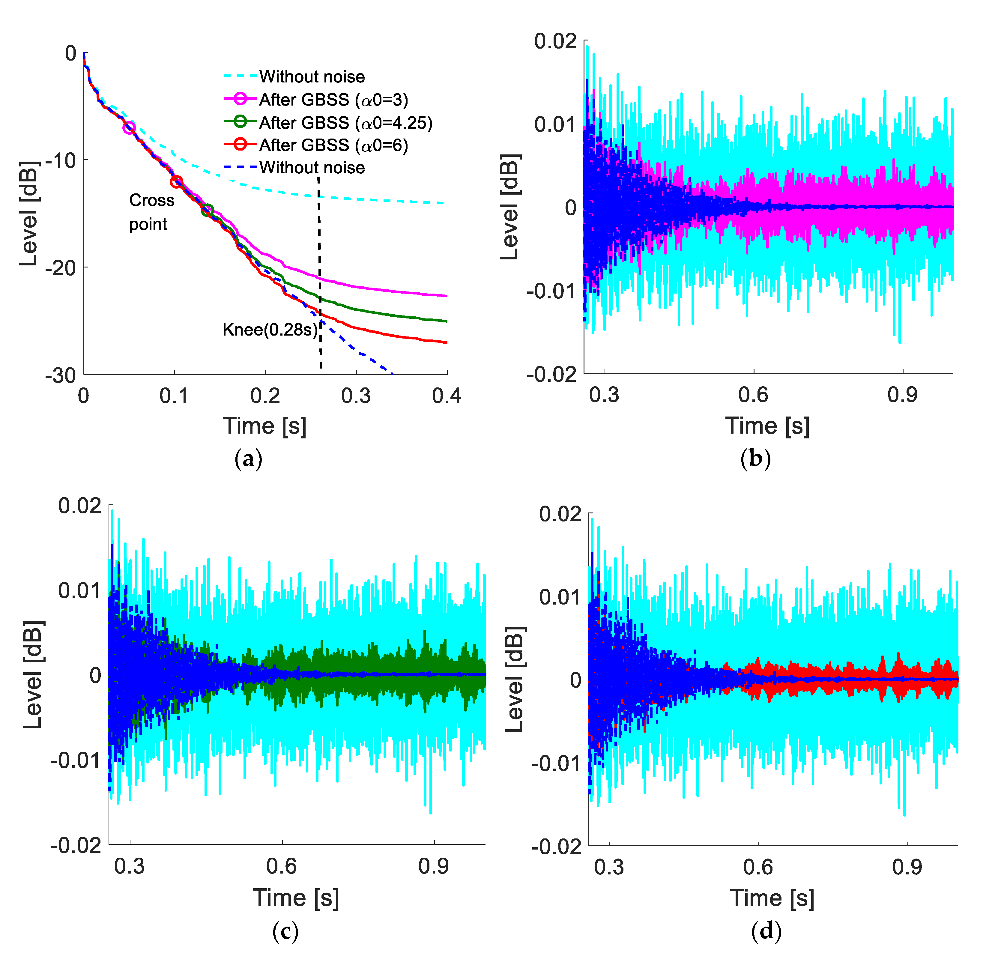
The EDCs of the de-noised RIRs with different values, , compared to the EDCs of the noisy RIRs and the reference RIRs in the time domain, are given in Figure 4. Observing the RIRs in the time domain, the noises were remarkably reduced for the applied GBSS algorithm with higher than 3. The higher the , the lower the remaining noise level. However, compared with the reference RIRs, the three values gave different performances in terms of the energy levels around the knee (about 0.28 s), leading to the variable performance to the generated EDCs. Observing the EDCs presented in Figure 4a, compared to the other two values, a value of 3 resulted in the worst dynamic range improvement. The amplitudes of the de-noised RIRs presented in Figure 4b were higher than the reference RIR at the knee. In such cases, much of the noise was removed, but not completely. Further increasing the value to 4.25 resulted in a decrease in the amplitudes at the knee until the energy levels were almost equal to the reference RIR around the knee (seen Figure 4c), yielding the largest dynamic range improvement (about −13 dB). At the same time, the EDC was overlapped with the reference before a cross point at the decay level −15 dB. In this regard, the cross point was called the critical point for the largest dynamic range obtained using the optimal over-subtraction factor . For a higher value of 6, though the noise levels were obviously reduced, the amplitudes around the knee decreased significantly, as shown in Figure 4d. Relative energy loss occurred at the original noisy signal around the knee, causing the corresponding EDC to be divided from the reference EDC to drop below the decay curve in the range of −15 dB to −24 dB. As a result, the estimated decay level at the corresponding cross point is smaller than the reference results. Most important is that the reverberation decay rate was degraded more severely than the reference one.
It was observed that the processing of RIR de-noising showed a strong dependence on the over-subtraction factors of of the GBSS algorithm. The performance showed that changing led to different cross points with the reference EDCs, and de-noised EDCs had a tremendous relationship with the reduced noise levels in noisy RIRs. On the other hand, the cross point located at the de-noise EDCs did not extend to the critical point until the noise levels around the knee were removed. On the other hand, the reverberation decay part of the signal would be lost using an value higher than the optimum, leading to a decay rate distortion at the knee and causing more significant deviations of the EDCs relative to the reference EDCs. Furthermore, the optimal factors providing the best results regarding the dynamic range improvements were variable for different noise levels. For example, for the applied optimal factor, 4, the dynamic range improvement was larger than 20 dB when the noise level was lower than −60 dB while a 15-dB improvement was achieved using 4.25 at a noise level of −45 dB.
4.3. Over-Subtraction Factor for the Octave Band RIRs and Different Noises
Because the most promising factors of the GBSS applied to RIRs with different noise levels are changed, and the dynamic range obtained was varied, it was essential to find the rule to choose the factors for different situations. Hence, the three measured RIRs with low noise levels, mentioned in Section 3.1, filtered in octave bands, convoluted with white noise and pink noise, with noise levels ranging from −65 dB to −40 dB, were used to determine the optimal factors. Based on the study above, removing the noise levels around the knee estimated from RIR contributed to the largest dynamic range improvement. In this case, the factors set in the GBSS were the most promising. The acoustic parameters calculated from the EDCs of the filtered RIRs in the octave bands were used to verify the results and guarantee the accuracy of the applied optimal factors, leading to no distortion of the EDCs during the noise subtraction process using the GBSS. Considering the optimal factors determined using the knees obtained with the compensation method, the corresponding RTs were compared with the reference RTs. The RTs calculated at the critical point positioned on the de-noised EDCs were compared with the values of the compensation method and the reference results to ensure that the achieved decay levels at the critical points were the best. At the same time, EDT, T15, and T20 were used to verify the GBSS algorithm and it was compared with the reference results, as listed in Table 2.
The EDCs generated from the RIRs of the meeting room filtered in the octave bands with noise levels of −60 dB are presented in Figure 5; the noise level estimated from the RIRs in each frequency band for the convoluted white noise remained the same as the noise levels of the pink noise. In this case, the knees located at the EDCs obtained using the S–T–C method were similar in each frequency band. In addition, the largest difference of the knee estimated at the EDCs for the pink noise and the white noise was 0.02 s in the octave band at 2000 Hz, causing an approximately 1.5 dB difference in the dynamic EDC ranges. However, the EDCs have a slight, but visible, deviation from the reference EDCs at the knees, and the maximum difference of the decay level was 2 dB.
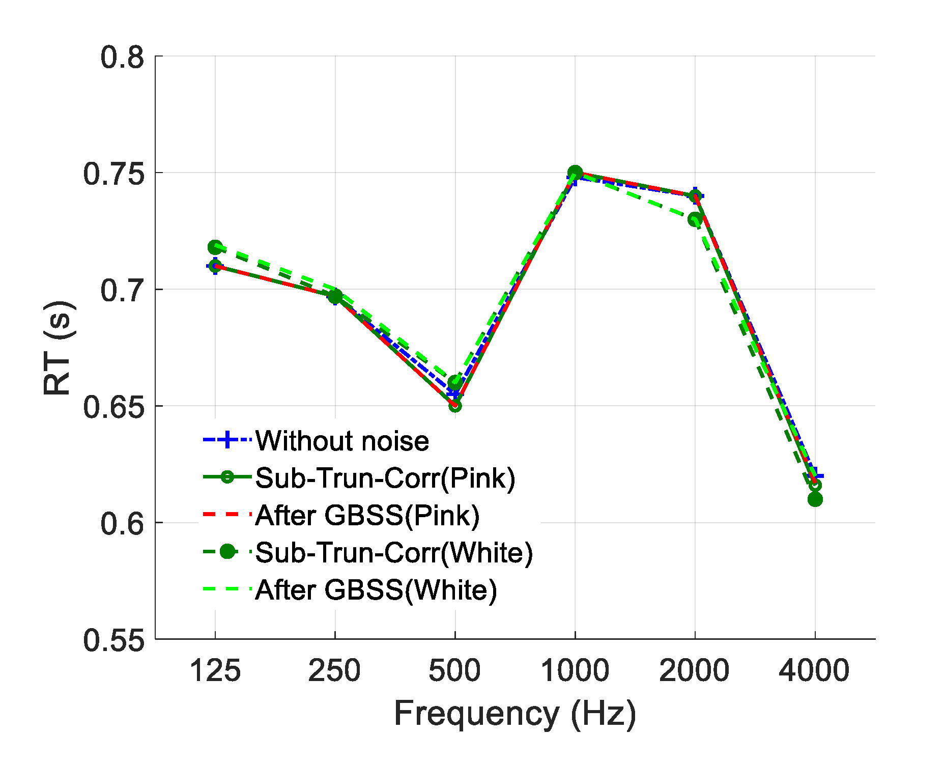
Figure 6 illustrates a comparison of the GBSS with the reference and compensation methods for RT estimation at critical points of white and pink noise. Compared to the reference results, the maximum deviation of the RTs for the GBSS algorithm was 0.13 s at 2000 Hz, and the dynamic range improvement of white noise compared to pink noise was about 2 dB. The compensation method generally produced similar results to the GBSS algorithm. This is why the knee can be used as the endpoint for the EDCs obtained using the compensation method, but is not adopted as the endpoint for EDCs with the GBSS algorithm. On the other hand, the EDCs are coincidental with the reference EDCs above the critical points positioned above the knees. At the same time, there was no apparent deviation of the three EDCs at the critical points.
The ranges from −5 dB to the decay levels estimated at the critical points were used to estimate the RTs presented in Table 2. T20 was considered for comparison at a noise level of −60 dB because the decay levels estimated at the critical points from the EDCs with two noises were independently in the range of −26 dB to −35 dB. In contrast, T15 was used when the noise level was −50 dB. The maximum differences of EDT and T20 was 0.006 s and 0.007 s, respectively. The deviation between the de-noised EDCs and the reference EDCs was approximately 0.01 dB. The critical points depended strictly on the over-subtraction factor to decide the improved decay levels of the dynamic range, and the accuracy of the produced reverberation decay rates. Over-subtraction factor α for the segment SNR achieved the best dynamic range improvement with the best value, connecting the estimated SNR at the filtered RIRs with the octave band, as shown in Figure 7a,b. The estimated SNRs and the optimal factors applied to the situation presented in Table 2 gave the same results. The values were 3.75 for frequency bands lower than 500 Hz when the estimated SNRs were higher than 30 and 4 for the frequency band higher than 500 Hz when the estimated SNRs were higher than 25. Consequently, the similar results of the two noises showed that the GBSS algorithm does not depend on the noise type. In applying optimal factors, the processing of the noise subtraction to achieve the best dynamic range, leading to no or minimal degradation of the reverberation decay, is reliable for implementing the RIRs.
An extension analysis was applied to three broadband-measured RIRs with two types of added noise (pink and white noises) at noise levels ranging from −40 dB to −65 dB. Figure 7c shows that the optimal factors of in the range of 3.75 to 5 depended on the SNR estimated in the octave bands. The higher the SNR, the lower the over-subtraction factor of . The optimal for an SNR higher than 30 was 3.75, 4 for an SNR higher than 24, and 4.25 for an SNR in the range from 10 to 24. Figure 7d shows the mean dynamic range improvements achieved in the octave bands by applying the most reliable optimal factor of , ranging from 3.75 to 4.25 for an SNR higher than 10. The dynamic range improvement achieved for noise levels lower than −60 dB was around 15 dB to 20 dB. The dynamic range decreased slightly with an increasing noise level, up to −40 dB, contributing to about a 13 dB improvement in the mean dynamic range. In most cases, the reverberation decay range could be extended to −10 dB. The deviation of the improvement was less than 2 dB, and the mean value and deviation of the noise level reduction were approximately 9 dB and 2.5 dB, respectively.
When the SNR is lower than 10, the applied optimal factors of were higher than 4.5, and the noise levels estimated at the frequency bands were lower than 40 dB. In this case, the mean improved dynamic range of the EDC ranged from 3 dB to 8 dB, causing the decay range for calculating the RT to be less than 10 dB. When the noise levels were higher than −40 dB, leading to similar poor results in the mean dynamic range improvement, approximately 5 dB, most of the SNRs estimated in the octave band were lower than 10. The application of the GBSS algorithm did not lead to a significant change in the dynamic range improvement when the SNRs in the octave bands were lower than 10.
The application of the GBSS algorithm did not lead to a significant change in dynamic range improvement when the SNRs of the octave bands were lower than 10. The optimal factors do depend on the SNRs instead of on the steady noise types and levels. The recommended spectral flooring parameter and over-subtraction factor α with different desired of the GBSS algorithm contributed to significant effects on both the dynamic range improvement and the noise floor reduction when the SNRs were estimated at frequency bands higher than 10. When de-noising the measured RIRs with real ambient noise, the used could be smaller than the optimal factor. A threshold of 0.25 is recommended for lowering the risk of signal over-subtraction regarding the difference in the dynamic range being smaller than 1 dB.
Applying the GBSS algorithm assumes that noise affects the entire spectrum of the signal equally. Over-subtraction factor α subtracts an overestimation of noise over the whole range. Although the noise affects the RIRs uniformly across the entire spectrum, the energy distribution in the frequency bands varies, leading to significantly different estimated SNRs of the RIRs filtered in the octave band. Thus, the factors of are significantly influenced by the SNRs in each frequency band and are estimated from the filtered noisy RIR. Hence, setting the optimal factors of the variable depends on the estimated SNR of the original RIR filtered in frequency bands instead of applying the same constant value of for every frequency band.
4.4. GBSS Method in Measured RIRs with Natural Ambient Noise
In the preceding sections, with the fixed spectral flooring parameter, the optimal factor , leading to the best dynamic range improvement, depended on the estimated SNRs of the filtered RIRs in the frequency bands presented in Figure 7c. The optimal spectral flooring parameter, β, depended on the averaged posterior SNR of the input signal [21,24]. Extensive experiments at noise levels higher than −40 dB were performed to set β = 0.001 at SNR >= 0 while β = 0.05 at SNR < 0. The best de-noising results were obtained using the optimal sets of factors that were conducted in two normal rooms with real ambient noise. In this part, the reference RIRs represent the measured RIRs with a noise level of −60 dB, while the noisy RIRs mean the RIRs were noise levels of −40 dB and −46 dB, separately. A detailed comparison of the GBSS algorithm with the noise compensation method and reference RIRs in terms of the EDCs, EDT, and RTs of the measured RIRs filtered in the octave bands showed that the optimal factors could be valid for actual applications. The generated EDCs at 250 Hz and 2 kHz were taken as examples to compare the results of the EDCs given in Figure 8. The optimal factors of applied for the two rooms in the octave bands were different. The value used in room A was 4.25 because of the estimated SNRs of the filtered RIRs in octave bands ranged from 12 to 18, and a factor of was 4 was used for room B because the estimated SNRs of the filtered RIRs in the octave bands ranged from 24.5 to 28. The de-noised EDCs were almost identical to the reference EDCs and the compensated EDCs were above the critical point and are indicated by the dash–dotted vertical line. The reverberation decay ranges were obviously extended using the optimal factors. The mean dynamic range improvements for rooms A and B were 12 dB and 14.4 dB, respectively. The mean noise levels reductions for rooms A and B were approximately 7.8 dB and 8.5 dB, respectively.
Table 3 lists the parameters of the EDT and RTs estimated at critical points using the optimal factors for the two rooms, compared with the reference results. The overall differences of the RTs estimated at the critical points, and the EDT of the frequency bands estimated at the de-noised EDCs, were small compared to the reference RIRs and the compensation method. The fluctuations caused by the GBSS algorithm had slight effects on the EDCs, leading to minor deviations in the early reverberation decays. The maximum relative errors of the EDTs for rooms A and B were 0.89% at an octave band of 500 Hz and 1.3% at an octave band of 1000 Hz, respectively. The corresponding time deviations were 0.011 s and 0.007 s, respectively. The maximum relative errors of the RT were 1.09% for room A at an octave band of 1000 Hz and 0.89% for room B at an octave band of 500 Hz. The corresponding time deviations were 0.015 s and 0.007 s, respectively. A comparison with the noise compensation method showed that the GBSS algorithm produced slightly better results when the optimal factors were applied. The mean relative errors of the EDT and RTs were 0.41% and 0.42% using the GBSS algorithm, respectively, whereas the corresponding values were 0.59% and 0.48% using the noise compensation method.
The relative errors of the RTs and EDT presented in Figure 9 showed that the optimal factors of the GBSS algorithm had a significant impact on the RIR de-noising. Nevertheless, the EDT calculated from the de-noised EDCs in the same octave bands were smaller than the reference ones, which illustrated that the EDCs went below the reference EDCs, leading to minimal degradation of the reverberation decay. The value of the factor was acceptable because the decay rate was not degraded.
The GBSS method with the optimal factors given in Figure 7c was valid for the measured RIRs. Although the relative errors of the RTs and EDT estimated by the noise compensation were within the limits and had a barely just noticeable difference [33], the method was sensitive to the correction term, requiring sophisticated procedures for a truncated time estimation [25]. Overall, the GBSS method is simple to implement with a solid flexibility to adapt to random noise by adjusting the over-subtraction factors according to the SNRs in the frequency bands instead of using a constant factor. The GBSS algorithm with these promising factors provides a good compromise between the noise reduction and the distortion of the RIR for acoustic parameter estimation.
5. Conclusions
This study examined the possibility of implementing the GBSS algorithm in de-noising RIRs to extend the reverberation decay range of the corresponding EDCs. Furthermore, a detailed analysis of the optimal set factors of the spectral subtraction algorithm, including the over-subtraction factor and the spectral flooring factor that could provide the most significant dynamic range improvement in the EDCs, was performed.
In regards to the dynamic range improvement in EDCs without distorting the quality of the RIRs, experiments were conducted in measured RIRs with artificial noise and natural ambient noise. The optimal sets of factors for de-noising the RIRs filtered in the octave bands by β 0.001 at SNR >= 0, and 0.05 at SNR < 0, while the over-subtraction factor α was calculated from Equation (2). Furthermore, the factor in Equation (2) depends on the estimated SNR of the RIRs filtered in the octave band, given in Figure 7c. The results showed that the improved dynamic range strictly depends on factor . If the values are lower than the optimum, a smaller dynamic range improvement compared to the best results is provided; in this case, the level is acceptable because no degradation occurs to the reverberation decay rate. On the other hand, if the value is too high, a loss of the original signals that appears in the RIRs will distort the reverberation decay rates. Therefore, it is essential to find the optimal to prevent the signal over-subtraction in the de-noising processing and minimize degradation on the reverberation decay.
The GBSS algorithm showed excellent significance in de-noising the RIRs when the noise levels were lower than −40 dB. The optimal was suggested in the range of 3.75 to 4.25 for different SNRs greater than 10. As a result, the mean dynamic ranges were improved by approximately 13 dB and even by 20 dB. Moreover, the noise levels were reduced by around 8 dB. When the estimated SNRs were lower than 10, the improved dynamic range was less than 8 dB using the optimal higher than 4.5, causing the EDC estimation decay range to be less than 10 dB, which contributes fewer effects to de-noising the RIRs regarding the dynamic range improvement. In applying the optimal sets of the factors to real measured noisy RIRs, the estimated RTs and EDT gave a somewhat more stable result in some cases compared to the compensation method.
Overall, the GBSS algorithm is simple to implement with substantial flexibility to improve the dynamic range of EDCs automated by adjusting the over-subtraction factors of , based on the different SNRs, instead of subtracting noise levels with a constant estimated noise level for the entire RIRs. Moreover, the GBSS algorithm using optimal factors has significant effects on de-noising the RIRs to extend the dynamic range of the EDCs and decrease the estimation errors in RTs caused by the noise levels.
Further work on de-noising the RIRs addresses two aspects. First, because the GBSS algorithm required noise to be stationary or a slowly varying process, a development of the algorithm must be considered for real-world cases with non-stationary background noise. Second, improving the algorithm to render musical noise perceptually inaudible by taking into account the properties of human auditory systems should be studied.
Author Contributions
C.-M.L. gave academic guidance to this research work and revised the manuscript. M.C. designed the core methodology of this study, programmed the algorithms, carried out the experiments, and drafted the manuscript. Both authors have read and agreed to the published version of the manuscript.
Funding
This research received no external funding.
Institutional Review Board Statement
Not applicable.
Informed Consent Statement
Not applicable.
Data Availability Statement
Not applicable.
Conflicts of Interest
The authors declare no conflict of interest.
References
- ISO 140: Acoustics—Measurement of Sound Insulation in Buildings and of Building Elements; International Organization for Standardization: Geneva, Switzerland, 1998.
- ISO 354: Acoustics—Measurement of Sound Absorption in a Reverberation Room; International Organization for Standardization: Geneva, Switzerland, 2003.
- ISO 17497-1: Acoustics—Sound-Scattering Properties of Surfaces—Part 1: Measurement of the Random-Incidence Scattering Coefficient in a Reverberation Room; International Organization for Standardization: Geneva, Switzerland, 2006.
- Sant’Ana, D.Q.; Zannin, P.H.T. Acoustic evaluation of a contemporary church based on in situ measurements of reverberation time, definition, and computer-predicted speech transmission index. Build. Environ. 2011, 46, 511–517. [Google Scholar] [CrossRef]
- Cabrera, D.; Xuan, J.Y.; Guski, M. Calculating Reverberation Time from Impulse Responses: A Comparison of Software Implementations. Acoust. Aust. 2016, 44, 369–378. [Google Scholar] [CrossRef]
- Schroeder, M.R. New method of measuring reverberation time. J. Acoust. Soc. Am. 1965, 37, 409–412. [Google Scholar] [CrossRef]
- Morgan, D.R. A parametric error analysis of the backward integration method for reverberation time estimation. J. Acoust. Soc. Am. 1997, 101, 2686–2693. [Google Scholar] [CrossRef]
- Janković, M.; Ćirić, D.G.; Pantić, A. Automated estimation of the truncation of room impulse response by applying a nonlinear decay model. J. Acoust. Soc. Am. 2016, 139, 1047–1057. [Google Scholar] [CrossRef]
- Lundeby, A.; Vigran, T.E.; Bietz, H.; Vorländer, M. Uncertainties of Measurements in Room Acoustics. Appl. Acoust. 1995, 81, 344–355. [Google Scholar]
- Ćirić, D.G.; Janković, M. Correction of room impulse response truncation based on a nonlinear decay model. Appl. Acoust. 2018, 132, 210–222. [Google Scholar] [CrossRef]
- Venturi, A.; Farina, A.; Tronchin, L. On the effects of pre-processing of impulse responses in the evaluation of acoustic parameters on room acoustics. J. Acoust. Soc. Am. 2013, 133, 3224–3231. [Google Scholar] [CrossRef]
- Hirata, Y. A Method of Eliminating Noise in Power Responses. J. Sound Vib. 1982, 82, 593–595. [Google Scholar] [CrossRef]
- Guski, M.; Vorländer, M. Comparison of noise compensation methods for room acoustic impulse response evaluations. Acta Acust. Acust. 2004, 100, 320–327. [Google Scholar] [CrossRef]
- ISO 3382–1: 2009, Acoustics—Measurement of Room Acoustic Parameters—Part 1: Performance Spaces; International Organization for Standardization: Geneva, Switzerland, 2009.
- Karjalainen, M.; Antsalo, P.; Makivirta, A.; Peltonen, T.; Valimaki, V. Estimation of modal decay parameters from noisy response measurements. J. Audio Eng. Soc. 2002, 50, 867–878. [Google Scholar]
- Noisternig, M.; Carpentier, T.; Szpruch, T.; Warusfel, O. Denoising of directional room impulse responses measured with spherical microphone arrays. In Proceedings of the 40th Annual German Congress on Acoustics (DAGA), Oldenburg, Germany, 10–13 March 2014; pp. 600–601. [Google Scholar]
- Massé, P.; Carpentier, T.; Warusfel, O.; Noisternig, M. Denoising Directional Room Impulse Responses with Spatially Anisotropic Late Reverberation Tails. Appl. Sci. 2020, 10, 1033. [Google Scholar] [CrossRef] [Green Version]
- Ðorðe, M.D.; Dejan, G.Ć.; Bratislav, B.P. De-Noising of a Room Impulse Response by Applying Wavelets. Acta Acust. United Acust. 2018, 104, 452–463. [Google Scholar]
- Kim, W.; Kang, S.; Ko, H. Spectral subtraction based on phonetic dependency and masking effects. IEEE. Proc. Vis. Image Signal Process. 2000, 147, 423–427. [Google Scholar] [CrossRef]
- Chu, W.T. Comparison of Reverberation Measurements Using Schröder’s Impulse Method and Decay—Curve Averaging Method. J. Acoust. Soc. Am. 1998, 63, 1444–1450. [Google Scholar] [CrossRef] [Green Version]
- Boll, S.F. Suppression of Acoustic Noise in Speech using Spectral Subtraction. IEEE Trans. Acoust. Speech Signal Process. 1979, 27, 113–120. [Google Scholar] [CrossRef] [Green Version]
- Simard, Y.; Bahoura, M.; Roy, N. Acoustic Detection and Localization of whales in Bay of Fundy and St. Lawrence Estuary Critical Habitats. Can. Acoust. 2004, 32, 107–116. [Google Scholar]
- Lebart, K.; Boucher, J.M. A new method based on spectral subtraction for speech dereverberation. Acta Acust. United Acust. 2001, 87, 359–366. [Google Scholar]
- Wei, D.; Nagata, Y.; Aketagawa, M. Suppression of noise in modulation frequency range of interferometer using spectral subtraction method. Opt. Commun. 2020, 475, 126–294. [Google Scholar] [CrossRef]
- Lin, T.T.; Yao, X.K.; Yu, S.J.; Zhang, Y. Electromagnetic Noise Suppression of Magnetic Resonance Sounding Combined with Data Acquisition and Multi-Frame Spectral Subtraction in the Frequency Domain. Electronics 2020, 9, 1254. [Google Scholar] [CrossRef]
- Hu, Y.; Loizou, P.C. Subjective comparison and evaluation of speech enhancement algorithms. Speech Commun. 2007, 49, 588–601. [Google Scholar] [CrossRef] [PubMed] [Green Version]
- Loizou, P.C. Speech Enhancement: Theory and Practice, 2nd ed.; Taylor and Francis: Boca Raton, FL, USA, 2013. [Google Scholar]
- Berout, M.; Schwartz, R.; Makhoul, J. Enhancement of Speech Corrupted by Acoustic Noise. In Proceedings of the IEEE International Conference on Acoustics, Speech, and Signal Processing, Washington, DC, USA, 2–4 April 1979; Volume 4, pp. 208–211. [Google Scholar] [CrossRef]
- Cohen, I. Noise spectrum estimation in adverse environments: Improved minima controlled recursive averaging. IEEE Trans. Acoust. Speech Signal Process. 2003, 11, 466–475. [Google Scholar] [CrossRef] [Green Version]
- Doblinger, G. Computationally efficient speech enhancement by spectral minima tracking in sub-bands. In Proceedings of the 4th Euro Conference on Speech Communication and Technology, Madirid, Spain, 18–21 September 1995; Volume 2, pp. 1513–1516. [Google Scholar]
- Rabiner, L.; Sambur, M.R. Voiced-unvoiced-silence detection using the Itakura LPC distance measure. In Proceedings of the IEEE International Conference on Acoustics, Speech, and Signal Processing, Hartford, CT, USA, 9–11 May 1997; pp. 323–326. [Google Scholar] [CrossRef]
- Vary, P.; Martin, R. Digital Speech Transmission: Enhancement, Coding and Error Concealment; John Wiley & Sons: Chichester, UK, 2006. [Google Scholar]
- Hak, C.C.J.M.; Wenmaekers, R.H.C.; Luxemburg, L.C.J.V. Measuring room impulse responses: Impact of the decay range on derived room acoustic parameters. Acta Acust United Acust. 2012, 98, 907–915. [Google Scholar] [CrossRef] [Green Version]
- Kondoz, A.M. Digital Speech: Coding for Low Bite Rate Communication Systems, 2nd ed.; Wiley: Chichester, UK, 2004. [Google Scholar]
- Eastland, G.C.; Buck, W.C. Reverberation characterization inside an anechoic test chamber at the Weapon Sonar Test Facility at NUWC Division Keyport. J. Acoust. Soc. Am. 2016, 139, 2031. [Google Scholar] [CrossRef]
Figure 1.
Dynamic range improvement of the EDC between cross-point A at a noisy RIR and cross-point B at RIR after the GBSS.
Figure 1.
Dynamic range improvement of the EDC between cross-point A at a noisy RIR and cross-point B at RIR after the GBSS.

Figure 2.
Comparison of the noisy RIRs and de-noised RIR at 1 kHz by varying the noise spectral floor for a fixed value of . (a) The EDCs of the RIRs. (b) Power spectrum of the RIRs obtained using the FFT. (c,d) RIRs in the time domain.
Figure 2.
Comparison of the noisy RIRs and de-noised RIR at 1 kHz by varying the noise spectral floor for a fixed value of . (a) The EDCs of the RIRs. (b) Power spectrum of the RIRs obtained using the FFT. (c,d) RIRs in the time domain.

Figure 3.
Comparison of the noisy RIRs and de-noised RIR at 1 kHz by varying the noise over-subtraction for a fixed value of . (a,b) Generated EDCs of the RIRs. (c,d) De-noised RIRs with 4 and 6 in the time domain.
Figure 3.
Comparison of the noisy RIRs and de-noised RIR at 1 kHz by varying the noise over-subtraction for a fixed value of . (a,b) Generated EDCs of the RIRs. (c,d) De-noised RIRs with 4 and 6 in the time domain.

Figure 4.
De-noising effects at the knee with various factors of . (a) Comparison of the dynamic range at the cross point. (b–d) Comparison of the de-noised RIRs to the reference RIRs at the knee: factor of (b) 3, (c) 4.25, and (d) 6 applied.
Figure 4.
De-noising effects at the knee with various factors of . (a) Comparison of the dynamic range at the cross point. (b–d) Comparison of the de-noised RIRs to the reference RIRs at the knee: factor of (b) 3, (c) 4.25, and (d) 6 applied.

Figure 5.
De-noising effects using the optimal set factors of the GBSS on the RIRs of the meeting room with different added noises filtered at the octave bands. The red dotted line is the EDCs with the pink noise. The green dotted line is the EDCs with white noise.
Figure 5.
De-noising effects using the optimal set factors of the GBSS on the RIRs of the meeting room with different added noises filtered at the octave bands. The red dotted line is the EDCs with the pink noise. The green dotted line is the EDCs with white noise.

Figure 6.
Comparison of the RTs of the filtered RIRs at octave bands with pink noise and white noise with noise levels of −60 dB.
Figure 6.
Comparison of the RTs of the filtered RIRs at octave bands with pink noise and white noise with noise levels of −60 dB.

Figure 7.
Results of the optimal for different SNRs of three filtered RIRs in octave bands with two types of noise and various noise levels (−65 dB to −40 dB estimated in broadband RIRs). (a,b) Optimal for RIRs with noise levels −60 dB and corresponding SNRs. (c) Relationship of the optimal and SNR. (d) Dynamic range improvement.

Figure 8.
Effects of the GBSS algorithm and compensation method of the measured RIRs filtered in octave bands (250 Hz and 2 kHz): (a,b) comparison results for room A; (c,d) comparison results for room B.
Figure 8.
Effects of the GBSS algorithm and compensation method of the measured RIRs filtered in octave bands (250 Hz and 2 kHz): (a,b) comparison results for room A; (c,d) comparison results for room B.

Figure 9.
Comparison of the GBSS algorithm and the compensation method. (a) Reverberation time relative errors. (b) Early decay time relative errors.
Figure 9.
Comparison of the GBSS algorithm and the compensation method. (a) Reverberation time relative errors. (b) Early decay time relative errors.


Table 1.
Information of the measured rooms.
| Room Type | Room Size (m) | Volume (m3) | Temperature (°C) | Reference RT | ||
|---|---|---|---|---|---|---|
| Length | Width | Height | ||||
| Anechoic Chamber | 8.4 | 7.2 | 6.0 | 363 | 22.7 | 0.08 |
| Meeting Room | 16.5 | 4.35 | 9.95 | 714 | 23.2 | 0.67 |
| Hall | 16.5 | 11.5 | 9.0 | 1708 | 22.8 | 3.14 |
| Room A | 12.0 | 9.0 | 3.2 | 346 | 20.2 | 1.32 |
| Room B | 8.5 | 7.5 | 3.2 | 204 | 20 | 0.72 |
Table 2.
Comparison of RTs and EDT between the de-noised RIRs and the reference RIRs.
| Octave Band | Reverberation | Reference | Noise Level (−60 dB) | Noise Level (−50 dB) | ||
|---|---|---|---|---|---|---|
| Pink Noise | White Noise | Pink Noise | White Noise | |||
| 125 Hz | EDT(s) | 0.728 | 0.73 | 0.727 | 0.73 | 0.722 |
| T15(s) | 0.727 | 0.73 | 0.727 | 0.73 | 0.72 | |
| T20(s) | 0.727 | 0.73 | 0.727 | |||
| 250 Hz | EDT(s) | 0.677 | 0.677 | 0.676 | 0.676 | 0.676 |
| T15(s) | 0.739 | 0.739 | 0.738 | 0.74 | 0.74 | |
| T20(s) | 0.672 | 0.673 | 0.672 | |||
| 500 Hz | EDT(s) | 0.691 | 0.691 | 0.69 | 0.69 | 0.69 |
| T15(s) | 0.6 | 0.6 | 0.6 | 0.6 | 0.6 | |
| T20(s) | 0.626 | 0.627 | 0.624 | |||
| 1000 Hz | EDT(s) | 0.609 | 0.61 | 0.61 | 0.61 | 0.61 |
| T15(s) | 0.704 | 0.7 | 0.7 | 0.7 | 0.7 | |
| T20(s) | 0.717 | 0.71 | 0.71 | |||
| 2000 Hz | EDT(s) | 0.529 | 0.53 | 0.53 | 0.53 | 0.53 |
| T15(s) | 0.611 | 0.61 | 0.61 | 0.61 | 0.61 | |
| T20(s) | 0.707 | 0.7 | 0.7 | |||
| 4000 Hz | EDT(s) | 0.436 | 0.434 | 0.436 | 0.437 | 0.437 |
| T15(s) | 0.535 | 0.533 | 0.534 | 0.535 | 0.533 | |
| T20(s) | 0.614 | 0.61 | 0.613 | |||
Table 3.
Comparison of RTs and EDT between the de-noised RIRs and the compensated RIRs.
| Frequency /Hz | Parameter | Room A | Room B | ||||
|---|---|---|---|---|---|---|---|
| Reference | After GBSS | Compensation | Reference | After GBSS | Compensation | ||
| 125 Hz | EDT | 0.859 | 0.86 | 0.854 | 0.754 | 0.749 | 0.748 |
| RT | 1.048 | 1.059 | 1.04 | 0.848 | 0.848 | 0.84 | |
| 250 Hz | EDT | 1.026 | 1.023 | 1.022 | 0.639 | 0.638 | 0.637 |
| RT | 1.31 | 1.309 | 1.311 | 0.836 | 0.84 | 0.837 | |
| 500 Hz | EDT | 1.24 | 1.229 | 1.22 | 0.594 | 0.592 | 0.592 |
| RT | 1.18 | 1.182 | 1.17 | 0.785 | 0.792 | 0.787 | |
| 1000 Hz | EDT | 1.408 | 1.404 | 1.4 | 0.54 | 0.533 | 0.533 |
| RT | 1.467 | 1.451 | 1.465 | 0.657 | 0.661 | 0.657 | |
| 2000 Hz | EDT | 1.447 | 1.442 | 1.44 | 0.44 | 0.44 | 0.44 |
| RT | 1.427 | 1.426 | 1.419 | 0.541 | 0.54 | 0.541 | |
| 4000 Hz | EDT | 1.314 | 1.311 | 1.309 | 0.371 | 0.37 | 0.37 |
| RT | 1.313 | 1.311 | 1.297 | 0.486 | 0.485 | 0.482 | |
Publisher’s Note: MDPI stays neutral with regard to jurisdictional claims in published maps and institutional affiliations. |
© 2021 by the authors. Licensee MDPI, Basel, Switzerland. This article is an open access article distributed under the terms and conditions of the Creative Commons Attribution (CC BY) license (https://creativecommons.org/licenses/by/4.0/).
Share and Cite
MDPI and ACS Style
Chen, M.; Lee, C.-M. De-Noising Process in Room Impulse Response with Generalized Spectral Subtraction. Appl. Sci. 2021, 11, 6858. https://0-doi-org.brum.beds.ac.uk/10.3390/app11156858
AMA Style
Chen M, Lee C-M. De-Noising Process in Room Impulse Response with Generalized Spectral Subtraction. Applied Sciences. 2021; 11(15):6858. https://0-doi-org.brum.beds.ac.uk/10.3390/app11156858
Chicago/Turabian StyleChen, Min, and Chang-Myung Lee. 2021. "De-Noising Process in Room Impulse Response with Generalized Spectral Subtraction" Applied Sciences 11, no. 15: 6858. https://0-doi-org.brum.beds.ac.uk/10.3390/app11156858
Note that from the first issue of 2016, this journal uses article numbers instead of page numbers. See further details here.