Article

Analysis of the Landfill Leachate Treatment System Using Arima Models: A Case Study in a Megacity

by
Carlos Alfonso Zafra-Mejía
1,*,
Daniel Alberto Zuluaga-Astudillo
2 and
Hugo Alexander Rondón-Quintana
3
1
Grupo de Investigación en Ingeniería Ambiental-GIIAUD, Facultad del Medio Ambiente y Recursos Naturales, Universidad Distrital Francisco José de Caldas, Carrera 5 Este #15-82, Bogotá DC E-111711, Colombia
2
Especialización en Diseño y Construcción de Vías y Aeropistas, Escuela de Ingenieros Militares, Ejército Nacional de Colombia, Bogotá DC E-111611, Colombia
3
Facultad del Medio Ambiente y Recursos Naturales, Universidad Distrital Francisco José de Caldas, Bogotá DC E-110321, Colombia
*
Author to whom correspondence should be addressed.
Submission received: 6 July 2021 / Revised: 19 July 2021 / Accepted: 23 July 2021 / Published: 29 July 2021
(This article belongs to the Special Issue New Trends in Waste Management Models)

Abstract

:
Leachate has been reported as the most significant source of landfill pollution. Predicting the characteristics of untreated and treated leachate may be useful during optimal scheduling of leachate treatment systems. The objective of this paper is to show an analysis of the operation of a landfill leachate treatment system in a Latin American megacity (Bogota, Colombia) by means of auto-regressive integrated moving average (ARIMA) models. A comparative analysis of the leachate treated with respect to reference legislation is carried out. The influence of climate variables during the operation of the treatment system is also considered. The results suggest that the concentrations of heavy metals (HMs), BOD5, and COD in untreated leachate do not follow the same annual cycles observed for the quantity of solid waste disposed within the landfill. This difference is possibly associated with the hydraulic retention time (HRT) of the leachate inside the conduction and pre-treatment system (storage/homogenization ponds). The ARIMA analysis suggests an HRT of up to one month (AR = 1) for the HMs identified as indicators of untreated leachate (Cu, Pb, and Zn). It is noted that the removal efficiency of HM indicators of the operation of the leachate treatment plant (Fe and Ni) is probably conditioned by operations carried out over a period of one month (AR = 1). The high input concentration of these HM indicators may prevent changing their ARIMA temporal structure during leachate treatment. This is reflected in the low removal efficiencies for all HMs under study (average = 26.1%).

1. Introduction

The environmental impacts generated by population growth and concentration, including the significant increase in solid waste quantities, is one of the main problems facing cities worldwide [1,2]. This trend has a negative influence on public health and natural resources close to final disposal sites for municipal solid waste (MSW) [3]. In Latin American countries, landfills are the most common final destination for MSW [4]. One of the most significant environmental problems associated with this type of facility corresponds to the liquid waste generated during its operation and closure [5,6]. Leachate has become one of the main challenges of liquid waste treatment engineering, due to its high polluting loads (e.g., organic matter and heavy metals), and therefore it stands out as one of the areas of greatest interest during landfill management [7,8]. In Latin America, it is often reported that the technologies implemented for the leachate transport and treatment do not meet the technical conditions for controlling environmental pollution and public health concerns [9]. This increases the operating costs of treatment systems and puts future use of existing natural resources at risk [10].
Leachate has been reported as the most significant source of landfill pollution [11]. Thus, during the development and implementation of strategies to reduce the environmental impacts of landfills, the collection and treatment of leachate should be a priority [10]. Worldwide, there are several publications of research results and comprehensive reviews focused primarily on the generation, composition, characterization, and treatment of leachate [12,13]. Most of these publications focus on technological aspects of leachate treatment and prospects for future development [14]. However, most studies lack relevant information on time series analysis approaches to the physicochemical parameters considered during the operation of these leachate treatment systems (LTSs). Predicting the characteristics of untreated and treated leachate may be useful during optimal scheduling of LTSs. This will also be useful for maintaining stable performance during the operation of LTSs. In a few cases, staff experience and telemetry are sufficient to properly program and control the operation of these LTSs. Therefore, if future operation is to be optimally programmed, and the performance of LTSs improved, it is necessary to look for additional forecasting approaches from the time series of the measured chemical parameters. In this way, time series analyses of water quality parameters using auto-regressive integrated moving averages (ARIMA) models can be very useful.
The ARIMA models have been successfully used in research for analysis in wastewater treatment plants (WTPs), and are popular due to their simplicity and robust statistical properties [15,16,17]. ARIMA models also provide a powerful method for accurate and reliable results without significant calibration time [18,19,20]. ARIMA models study the possible relationship in time between current and past data and their errors. These characteristics have favoured the application of ARIMA models to forecast the different variables in many fields of engineering and science associated with water resources [21,22]. ARIMA models assume that the time series is generated from a linear process. This cannot be appropriate if the phenomenon under study is not linear, and indeed, this is what often happens in practice with real systems [23]. To overcome this weakness of ARIMA models with nonlinear time series, pre-processing techniques have been used [24]. For example, Maleki et al. [25] compared the performance of ARIMA (linear) and Artificial Neural Network (nonlinear) models to simulate time series of control parameters in a WTP. The results showed that ARIMA models were more accurate than Artificial Neural Network models in predicting daily concentrations of CO2, Cl, and Ca.
Studies on the use of ARIMA models in landfill leachate treatment systems are scarce. However, ARIMA models were used in various studies associated with water quality. For example, Lotfi et al. [26] used these models to study the temporal behaviour of water quality parameters (TSS, BOD5, and COD) in a WTP. These researchers reported that the ARIMA models were useful for improving efficiency in the WTP relative to BOD5 (R2 = 0.990). Ömer Faruk [27] also used ARIMA models to simulate water quality parameters of a basin in Turkey. This research properly simulated water quality parameters for 108 months. The correlation coefficients obtained between observed and simulated data for temperature, boron, and dissolved oxygen were 0.909, 0.902, and 0.893, respectively. Parmar and Bhardwaj [28] obtained satisfactory results when analysing parameters such as pH, BOD5, and COD in surface water bodies with ARIMA models. These researchers demonstrated the effectiveness of ARIMA models in analysing the temporal behaviour of these parameters and forecasting. Ahmad et al. [29] used these models to forecast conductivity, chlorine, and BOD5 of the Ganges River in India. Lastly, Taheri Tizro et al. [30] studied the modelling of water quality time series in a river with nine parameters. The results of this study showed the good performance of the proposed ARIMA models for the water quality estimation.
This research was developed in a landfill of a megacity in a developing country (Bogotá, Colombia). The metropolitan population for 2020 was 10.7 million, and an average of 6400 tons/day were discharged into the study landfill. This facility was located inside the megacity (southern zone), and its tropical mountain climate (2600 m.a.s.l.) was characterized by significant hourly variations in temperature (up to 12 °C). The leachate treated by the system under study was discharged into one of the three most important surface water sources of the megacity (Tunjuelo River). Worldwide, there is little research on the analysis of the functioning of LTSs in developing countries with this level of population and climate characteristics. This lack of knowledge, in part, motivated the development of this study.
The objective of this paper is to show an analysis of the operation of a landfill LTS in a Latin American megacity (Bogota, Colombia) by means of ARIMA models. The time series analyses correspond to chemical water quality parameters, measured at the inlet and exit of LTS. This study will be relevant to deepening knowledge in relation to the following aspects: (i) the temporal behaviour of landfill leachate in a megacity of a developing country, (ii) the influence of the climate conditions of the study site on the LTS, and (iii) the use of ARIMA models to detect potential problems and opportunities for improvement during the operation of landfill LTSs.

2. Materials and Methods
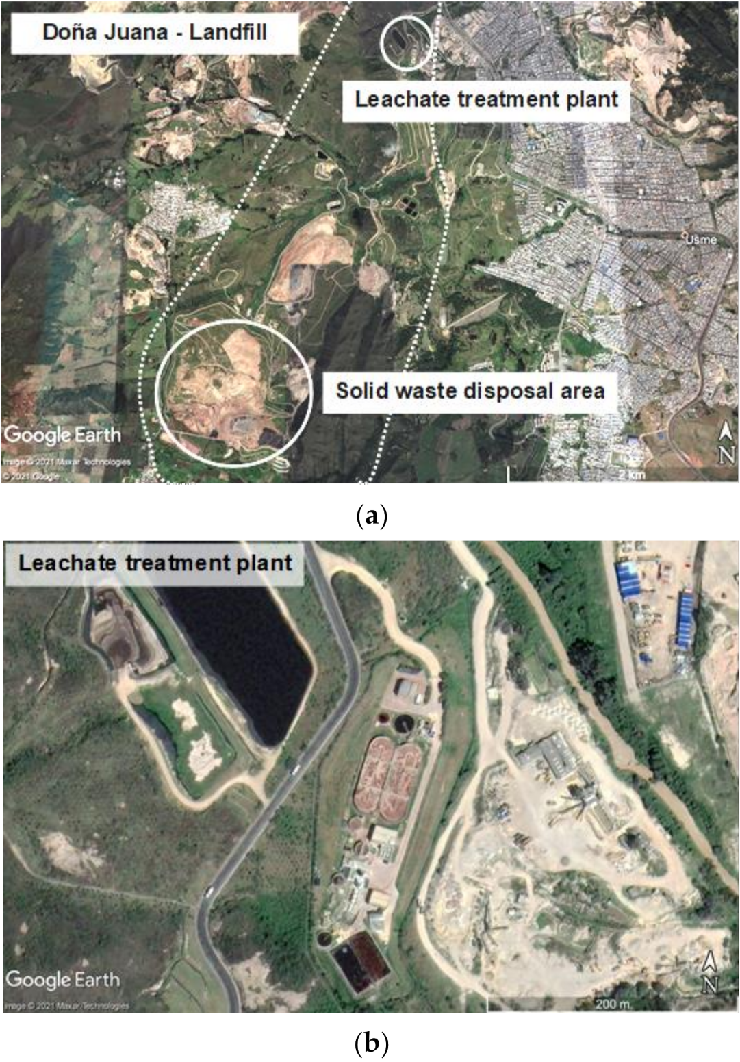
2.1. Study Site

The ‘Doña Juana’ landfill is in Bogota city, Colombia (4°31′18″ N; 74°07′44″). The climate in the landfill area is cold and dry (tropical mountain climate), with an average temperature of 13.6 °C. The annual distribution of rainfall has bimodal behaviour, with maximum values in April and October, and minimum values in January and July. The average annual rainfall in the study area is 799 mm. The landfill is located at an average elevation of 2758 m.a.s.l., and receives the MSW of 10.7 million people. The total area of the facility is 456 ha, of which about 40% is used as an MSW disposal area. The facility was divided into waste disposal zones, and during the study period Zone 8 was in operation. This disposal area had an area of 41 ha, an average depth of 40 m, and a storage capacity of 9.30 million tons of MSW (Figure 1). Between 700–800 compactor collecting trucks entered the landfill daily, which deposited an average of 6400 tons of MSW.
The storm water control in the closed areas of the landfill is carried out through a network of open stone-clad canals. There are also storm water channels on access roads, temporary discharge areas, and around the deposited MSW. The waste disposal area under study has a leachate collection and conduction system. This secondary system connects to a 304.8-mm diameter main conduction network, which then connects to four leachate storage and homogenization ponds. The landfill has a leachate treatment plant with a design flow rate of 26 L/s (Figure 1). In this regard, average operating flows are observed during the periods of increased and decreased rainfall of 20.6 L/s and 7.11 L/s, respectively. The leachate treatment is carried out by physic-chemical (coagulation and chemical precipitation) and biological (extended aeration with denitrification) processes. The maximum design conditions of the leachate treatment plant consider a load of 10,500 kg/day of BOD5, and concentrations of BOD5, TSS, and nitrogen of 15,000 mg/L, 2500 mg/L, and 2000 mg/L, respectively.

2.2. Information Collection

Daily water samples at the inlet and exit of the leachate treatment plant over a 12-year period (2003–2015) were collected. The parameters analysed were as follows: BOD5, COD, pH, N-NH4, Cd, Zn, Hg, As, Cu, Fe, Pb, Co, Cr, and Ni. The materials used during each sampling were as follows: digital field pH-meter (Hanna Instruments E-316), preservatives, amber bottles, microbiological bottles, refrigerator, buffer solutions, distilled water washing vessel, and a bucket. During each sampling, a bucket was initially filled with leachate, which was then removed to purge it. Subsequently, the bucket was filled again with leachate to obtain the corresponding sample. The pH-meter was calibrated with buffer solutions and measured in situ. Two aliquots were then packed in amber bottles of 1000 mL each. An aliquot was also packaged in a 100 mL microbiological sampling bottle, ensuring that there was no oxygen left in it. The containers were taken to a refrigerator, where they were kept at a temperature below 4 °C for later transport and laboratory analysis. The leachate samples collection followed the guidelines established by the Standard Methods for the Examination of Water and Wastewater [31].
Additionally, daily information on the quantity of MSW deposited in the study area was collected. This information was obtained using a scale installed at the entrance of the landfill. Lastly, daily rainfall and temperature information was collected from a weather station (4°28′52.7″ N; 74°7′34.6″ W) administered by the Institute of Hydrology, Meteorology, and Environmental Studies of Colombia (IDEAM). This monitoring station was located 2.29 km from the MSW disposal area under study.

2.3. Laboratory Analysis

The laboratory analyses were developed in accordance with the guidelines of the Standard Methods for the Examination of Water, and Wastewater [31]. The methods used for each parameter were as follows: BOD5, SM 5210 B, 4500 O, and C, Incubation Azide Modification; COD and SM 5220 C, Volumetric, Closed Reflux; NH4, SM 4500-NH3 B, and C, Titrimetric Method; and Cd, Zn, Hg, As, Cu, Fe, Pb, Co, Cr, and Ni, SM 3125 B, Inductively Coupled Plasma-Mass Spectrometry (ICP-MS) Method.

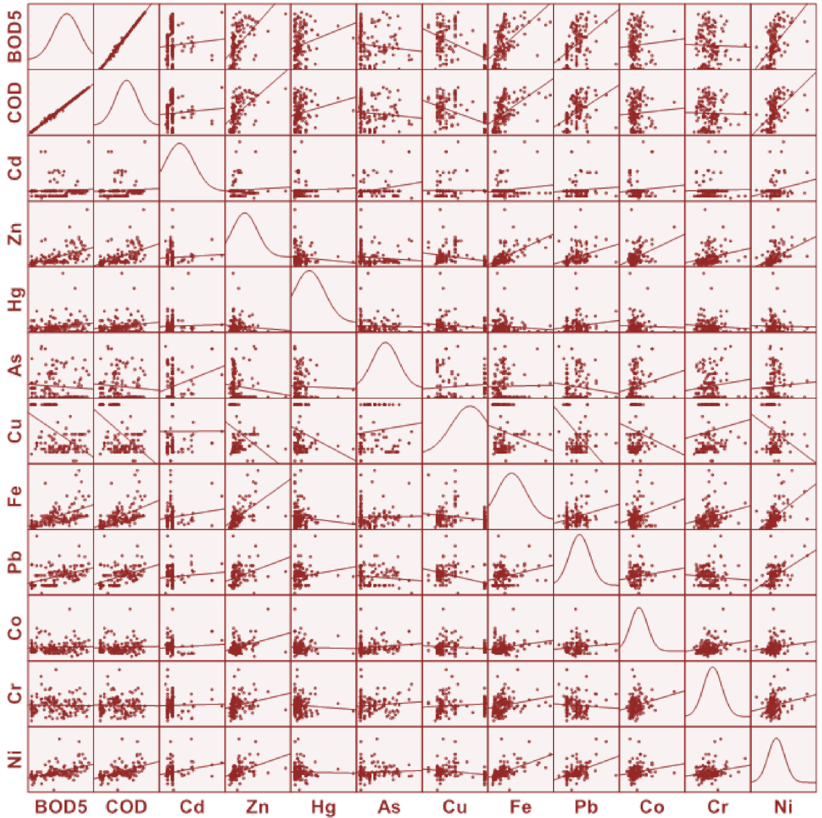
2.4. Information Analysis

The information analysis considered three phases. Phase 1: Daily information of all variables under study was aggregated to obtain time series on a monthly scale (2003–2015). A descriptive statistical analysis was performed to detect trends or anomalies in time series. The normal distribution of time series was evaluated by a Kolmogorov–Smirnov test (p-value > 0.05). Relationships between variables were also studied using Pearson’s correlation coefficient (r) to establish possible control parameters or indicators of the functioning of LTS. In this study, it was assumed that the parameters with the best correlations were those that possibly explained the functioning of LTS. A principal component analysis was also applied to complement the previous analysis.
Phase 2: A comparative analysis of the chemical parameters of leachate was carried out in relation to reference guidelines: Colombian Resolution 631 of 2015 [32] and Royal Spanish Decree 646 of 2020 [33]. Spanish legislation was selected in this study as it was more demanding compared to Colombian legislation, and was also adapted to the European context. The contaminant removal efficiency of the leachate treatment plant was also studied in accordance with the guidelines of Romero-Aguilar et al. [34]. Lastly, the influence of climate variables (rainfall and temperature) on leachate concentrations before and after the treatment plant was studied.
Phase 3: ARIMA models were developed using the iterative method of Box et al. [15], to study the chemical parameters time series of leachate before (untreated) and after (treated) the treatment plant. Daily data for all variables under study were averaged monthly. Thus, the time series considered for the ARIMA analysis were monthly. This time scale was also used to identify trends in the chemical parameters of untreated and treated leachate. The iterative stages reported by Box et al. [15] were considered in the development of ARIMA models: (i) model identification, (ii) parameter estimation, (iii) assumption verification, and (iv) model use. These stages were executed using the statistical software IBM-SPSS V.18.0. During the model identification stage, the stationarity of the time series was analysed. To obtain a stationary time series, if necessary, we used the square root and natural logarithmic transformations. In addition, the orders of the auto-regressive and moving average polynomials were determined, as well as the degree of differentiation to cancel the non-seasonality of the time series. The terms AR and MA of the stationary time series were obtained by analysing the patterns in the autocorrelation function (ACF) and partial autocorrelation function (PACF) diagrams [35]. This process involved several trial and error tests. The models identified were also contrasted with results from the expert modelling tool of the IBM-SPSS software [36]. Therefore, the orders ‘p’, ‘d’, and ‘q’ of the ARIMA models identified for each time series of chemical parameters under study were determined.
In the second stage, the parameters of the auto-regressive (ø1, …, øp or Lag 1, …, Lag p) and moving average (θ1, …, θp or Lag 1, …, Lag p) polynomials were determined for each model identified by the maximum likelihood method [35]. In this study, a constant was not included in ARIMA models when differentiation was applied [36]. Outliers were also not considered for the ARIMA models developed. In the third stage, the eight assumptions proposed by Box et al. [15] were verified, to select the best models for each time series. The goodness-of-fit of each ARIMA model was evaluated by the R2 value (determination coefficient). The suitability of modelling was assessed using the Ljung–Box (Q’) statistic. This is also recognized as the modified Box–Pierce statistic. This statistic tests the null hypothesis that there is no significant autocorrelation left in the model residuals, and provides an indication of whether the model is specified correctly. A p-value > 0.05 meant that the ARIMA model was properly specified to describe the correlation information in time series [37]. For models in a particular time series that passed the assumption verification stage, the Bayesian Information Criterion (BIC) was used to select the best model. The best model was selected when the BIC was the lowest [38]. Overall, in this study, the use of the BIC statistic was consistent, as the time series were generated from an ARMA process. This is in contrast to the Akaike and Akaike Corrected information criteria [39]. A residual analysis was performed after the modelling to ensure the normality of the residual, and no remaining autocorrelations or partial autocorrelations were detected. Lastly, the best-fit model was used to set the time series forecast values. Forecasting performance of the selected ARIMA models was evaluated based on mean absolute percentage error (MAPE), mean absolute error (MAE), and root mean square error (RMSE).

3. Results and Discussion

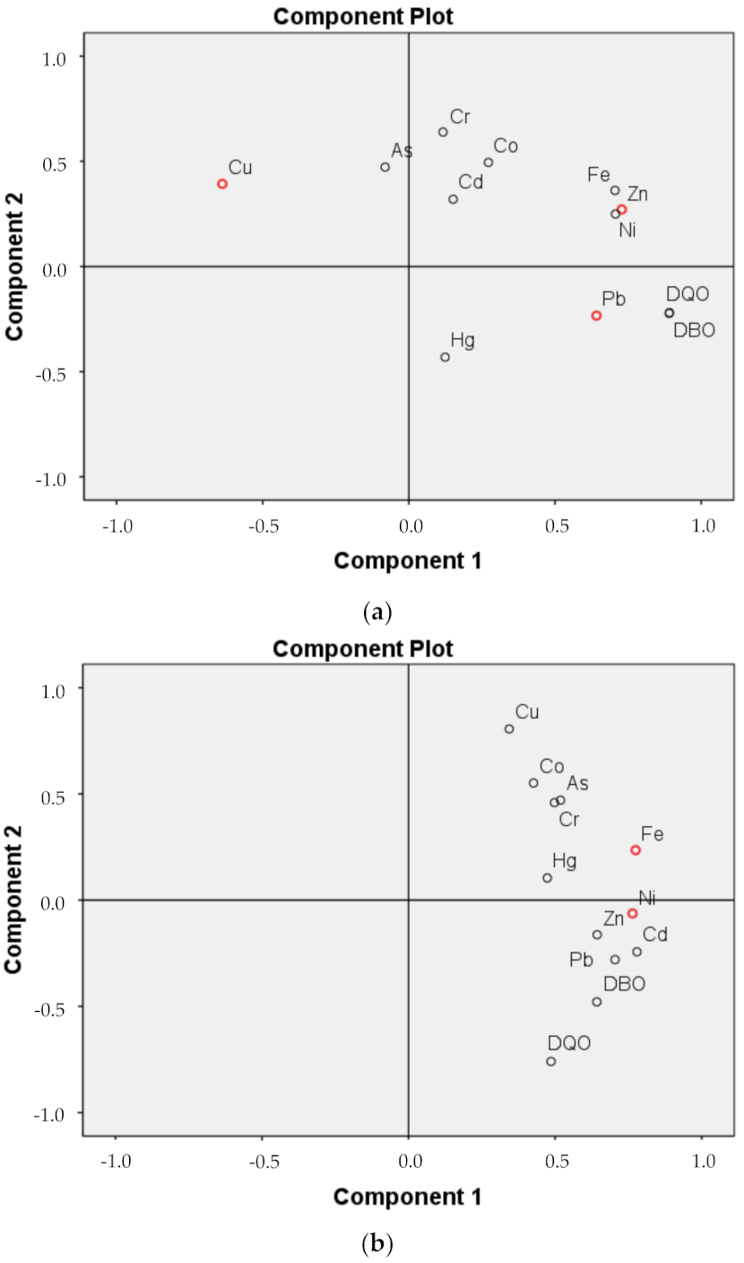
3.1. Untreated Leachate

A global comparative analysis with mature landfills [4,40,41,42,43,44,45,46] showed that, on average, the BOD5 (32.8–19,402 mg/L) and COD (2198–32,358 mg/L) concentrations in the study landfill were within the same range of variation (Table 1). However, concentrations of NH4, Cd, Hg, and Pb were, on average, 3.22, 1.21, 6.26, and 4.13 times higher compared to reference landfills, respectively. Indeed, the results suggested that these high concentrations of heavy metals (HMs) in leachate were possibly associated with the type of MSW disposed. This could also imply limitations on the access control of other types of MSW to the facility under study (e.g., industrial waste). The comparative analysis was performed with respect to mature landfills due to the analysis period considered in this study (13 years). However, the average BOD5/COD ratio (0.548) of the leachate could correspond to a young landfill [47]. Renou et al. [48] reported that concentrations of HMs and organic matter indicators were determining factors in the selection of leachate treatment technology, so the concentration of these parameters affected their removal efficiency.
The results showed significant correlations between climate variables and chemical parameters of untreated leachate. The climatic variable that showed the best correlations was temperature. Specifically, temperature showed negative correlations between ‘medium’ and ‘considerable’ with BOD5 (r = −0.709, p-value < 0.001) and COD (r = −0.709, p-value < 0.001). The findings suggested that, during periods of temperature increase, concentrations of BOD5 and COD in untreated leachate tended to decrease. Namely, during these periods of temperature increase, a lower volume of leachate was possibly generated, which allowed an increase in the hydraulic retention time (HRT) in the storage and homogenization ponds before its treatment. Moreover, increasing the HRT in the ponds possibly also increased the sedimentation of solids contained in the leachate. All of the above possibly resulted in a reduction in BOD5 and COD concentrations at the entrance of the leachate treatment plant. De Castro et al. [49] reported a similar trend in storage and homogenization ponds prior to leachate treatment. However, in the absence of storage and homogenization ponds, Renou et al. [48] reported that in the rainy periods the BOD5 and COD concentrations in untreated leachate tended to decrease (i.e., by dilution) compared to dry periods or temperature increases.
An analysis with Pearson’s coefficient showed that among the HMs, Cu, and Pb had the best correlations in untreated leachate (see Figure 2, and Table S1 in the supplementary information). These HMs had significant correlations between ‘medium’ and ‘very strong’ with Hg (r ≥ 0.940; p-values < 0.001), Cd (r ≥ 0.790; p-values < 0.001), and Co (r ≥ 0.763; p-values < 0.001). These HMs also had correlations between ‘weak’ and ‘medium’ with Zn (r ≥ 0.306; p-values < 0.001) and Cr (r ≥ 0.171; p-values < 0.001). In other words, this group of HMs (Cu, Pb, Hg, Cd, Co, Zn, and Cr) possibly had affinity in the origin, or were generated from the same type of MSW disposed in the landfill. Other HMs did not have significant correlations with Cu and Pb, but did have significant correlations with HMs from the previous group. This was the case with Ni, which showed significant correlations between ‘weak’ and ‘medium’ with Zn (r = 0.421; p-values < 0.001) and Cd (r = 0.408; p-values < 0.001). In this study, the previous correlations initially suggested Cu and Pb as the possible indicators of HMs contained in the untreated leachate. However, an analysis of principal components showed the following four groups in order of importance (determinant < 0.001): component 1 = Zn, Pb, Ni, and Fe (variance = 27.9%); component 2 = Cu and Cr (variance = 16.0%); component 3 = Cd and As (variance = 12.4%); and component 4 = Co and Hg (variance = 9.82%). Thus, Zn was also selected as a possible indicator of HMs in untreated leachate.
Additionally, BOD5 and COD concentrations had no significant correlations with the Cu and Pb concentrations (Figure 2). However, an analysis of principal components between the BOD5 and COD concentrations, and the concentrations of all HMs allowed visualizing a first component of four consisting of the following parameters and metallic elements (determinant < 0.001): COD, BOD5, Zn, Ni, Fe, Pb, and Cu (variance = 33.9%). Thus, it was observed that Zn was the metallic element of best correlation with the DBO5 and DQO concentrations in untreated leachate (BOD5-r = 0.516, p-value < 0.001; COD-r = 0.519, p-value < 0.001). The above also supported the selection of Cu, Pb, and Zn as possible HM indicators of the behaviour of the leachate untreated in this study. Figure 3a shows the HM indicators of untreated leachate on a diagram of two principal components, for better visualization. It was also observed that in each quadrant of the diagram an indicator HM was placed. Wdowczyk and Szymańska-Pulikowska [50] also used these three HMs as indicators of the pollution degree of untreated leachate in active and closed landfills in Poland.
The results of ARIMA modelling showed that the trend in HM concentrations was not to show a seasonal component: (p,d,q)(0,0,0). Namely, there was no annual cyclical behaviour in HM concentrations in untreated leachate (Table 2). Conversely, the model developed for the monthly MSW quantity disposed in the landfill showed a seasonal or cyclic component of one year: (p,d,q)(1,1,0). In this study, the results suggested that HM concentrations in untreated leachate did not follow the annual cycles observed in the MSW quantity disposed in the landfill. These differences in the temporal behaviour of HM concentrations in untreated leachate and in the MSW quantity disposed in the landfill were probably associated with the hydraulic retention time (HRT) of leachate in the transport system (pipeline) and pre-treatment (storage and homogenization ponds) under study. The results also showed that the BOD5 and COD concentrations did not have an annual cyclic component, such as that observed for MSW quantity disposed in the landfill. Indeed, instead of the quantity of disposed MSW, the studies report the following factors conditioning the leachate quantity and composition: landfill age, ambient air temperature, rainfall and permeability, depth, and temperature of the waste [51].
In relation to the concentrations of indicator HMs (Cu, Pb, and Zn), the findings showed that the term auto-regressive (AR) of the ARIMA models developed varied between 0–1 (Table 2). The other HMs under study had similar behaviour, except for As, which showed an AR = 2. These results suggested that the behaviour of HM concentrations in untreated leachate had a short memory. In other words, HM concentrations in untreated leachate were influenced by concentrations observed up to a month earlier. These results also suggested that the HRT of HMs in the leachate transport and pre-treatment system was probably up to one month, except for As, where the HRT was probably up to two months. There were studies that suggested a comprehensive increase in the HRT of untreated leachate to optimize the operation of treatment systems in the face of high pollutant concentrations. Specifically, it was suggested to extend the HRT of leachate in the waste cells and regulation ponds [52]. In relation to the organic matter content in untreated leachate, ARIMA analysis showed that memory was null (AR = 0). Namely, there were no influences from previous observations.
On the other hand, the results showed that the moving average (MA) term of ARIMA models developed for indicator HM concentrations was equal to one (MA = 1). In other words, the results suggested short fluctuations in the indicator HM concentrations in untreated leachate. These fluctuations in HM concentrations were probably up to one month. The other HMs under study also tended to show short fluctuations from the magnitude of their term MA, between 0–2 consecutive months (Table 2), except for Cd, which showed a variation of 11 consecutive months (MA = 11). In this study, the findings suggested Cd to be the HM with the greatest concentration variation in untreated leachate. Indeed, this suggested a greater occurrence of outliers in Cd concentration during the study period. The HMs with the least variation in concentration were As, Cr, and Ni (MA = 0), followed by Cu, Pb, Zn, Hg, and Fe (MA = 1). These variations were relative to the average concentration of each parameter during the study period.
Additionally, this difference in the term MA from the developed models also suggested that there were more difficult HMs to homogenize in untreated leachate ponds. The ascending order of homogenization in the ponds was possibly as follows: Group 1 = Cd; group 2 = Co; group 3 = Zn, Hg, Cu, Fe, and Pb; and group 4 = As, Cr, and Ni (Table 2). ARIMA analysis also suggested that organic matter (BOD5 and COD) could be in the third group of homogenization (MA = 1). The findings also hinted that the MSW disposal associated with groups 3 and 4 of HMs was possibly more uniform compared to the MSW disposal associated with Cd and Co. Table S2 shows the parameter estimates for the ARIMA model terms selected for the variables considered in the untreated leachate.

3.2. Treated Leachate

The comparative analysis with the Colombian guideline for wastewater discharge showed that, on average, COD was the only parameter that did not comply. This parameter showed concentrations 1.26 times higher than the Colombian limit (Table 1). However, there were periods in which other chemical parameters of the treated leachate also exceeded the established limits. The concentrations of Pb, Cr, Ni, Hg, and COD showed excesses during 6.25%, 27.8%, 11.8%, 0.69%, and 38.2% of the study time, respectively. Compared to the Spanish guideline, the results showed greater excesses. For example, COD concentrations exceeded the Spanish limit by an average of 100 times. The concentrations of Pb, Cr, Hg, BOD5, and COD showed excesses during 100%, 100%, 100%, 95.5%, and 94.2% of the study time, respectively. Indeed, in the last two years of study, a significant reduction in concentrations of BOD5 and COD was observed, possibly associated with landfill stabilization. On average, this reduction was 2.27 and 6.28 times, respectively. Bolyard and Reinhart [53] reported a similar trend during the stabilization of a MSW landfill.
The results showed significant correlations between climate variables and chemical parameters of treated leachate. The climate variable that showed the best correlations was temperature (Table S3). The temperature showed positive correlations between weak and medium with Co (r = 0.473; p-value < 0.001), As (r = 0.470; p-value < 0.001), Cr (r = 0.427; p-value < 0.001), Hg (r = 0.421; p-value < 0.001), Fe (r = 0.378; p-value < 0.001), and Ni (r = 0.232; p-value = 0.004). Moreover, temperature also showed a positive correlation between medium and considerable with Cu (r = 0.648; p-value < 0.001). In the treated leachate, findings showed better correlations between temperature and HM concentrations earlier than with COD. This trend was opposite compared to untreated leachate. In fact, HM concentrations in the treated leachate depended mainly on the treatment plant operation, rather than on the climate conditions. Al-Yaqout and Hamoda [54] reported the influence of climate factors on the leachate quality generated in a MSW landfill, which could also condition the functioning of their leachate treatment plant.
An analysis between HMs with Pearson’s coefficient showed that Fe associated the best correlations in treated leachate (Figure 4 and Table S3). This HM showed positive correlations between ‘medium’ and ‘considerable’ with Ni (r = 0.511, p-value < 0.001) and Cr (r = 0.629, p-value < 0.001). This HM also showed positive correlations between ‘weak’ and ‘medium’ with As, Zn, Cu, Cd, Hg, Pb, and Co (p-values < 0.001). Indeed, the previous correlations were conditioned by the type and efficiency of the leachate treatment plant under study. These correlations initially suggested Fe as the possible indicator of HMs during the operation of the leachate treatment plant under study. The Fe concentration in the treated leachate also showed positive correlations between ‘weak’ and ‘medium’ with COD (r = 0.279, p-value < 0.001) and BOD5 (r = 0.426, p-value < 0.001) concentrations. Thus, in treated leachate, there was probably similar behaviour between Fe and BOD5 concentrations. A principal component analysis allowed visualization of a first component of four, consisting of the following parameters and elements (determining < 0.001): Fe, Ni, Cd, Pb, Zn, BOD5, As, and COD (variance = 36.6%). In this way, Ni was also selected as a possible operation indicator of the leachate treatment plant under study. El-Gendy et al. [55] also used Fe and Ni as operating indicators of a leachate treatment plant for HM removal. Figure 3b shows the indicator HMs of the treated leachate on a diagram of two principal components, for better visualization. It was also observed that in each quadrant of the diagram was located a HM indicator (Fe and Ni).
The findings of ARIMA modelling in treated leachate showed that HM concentrations did not have a seasonal component: (p,d,q)(0,0,0). In other words, there was no annual cyclical component in the HM concentrations of treated leachate (Table 2), except for Co, which showed a one-year cycle in its concentrations: (p,d,q)(1,0,1). This annual cycle was also observed for MSW disposed in the landfill. In general, the results suggested that the HM concentrations in treated leachate depended mainly on the treatment plant operation rather than on the MSW quantity disposed in the landfill. The findings also suggested a similar seasonal trend between HM concentrations in treated and untreated leachate. Namely, there was no evidence of a seasonal component in the HM concentrations before and after the leachate treatment plant under study, except for Cd and Co in untreated and treated leachate, respectively.
In relation to the HM concentrations indicators of the leachate treatment plant (Fe and Ni), the results showed ARIMA models with a term AR = 1. The Cr also showed similar results (Table 2). Moreover, Fe (7.78 mg/L), Cr (0.455 mg/L), and Ni (0.390 m/L) were the HMs which tended to show the highest concentrations in the treated leachate (Table 1). Thus, the findings suggested that concentrations of these HMs were influenced by the concentrations observed during the month immediately preceding. Namely, the removal of these HMs at the leachate treatment plant was possibly conditioned by operations performed over a one-month period. This was also probably influenced by the high concentrations observed at the inlet of the leachate treatment plant: Fe = 97.2 mg/L, Cr = 0.717 mg/L, and Ni = 0.488 m/L. On average, Carvajal and Cardona [56] also reported that the HMs with the highest concentrations in leachate prior to treatment were Fe (200–1000 mg/L), Ni (0.050–2.0 mg/L), and Cr (0.020–1.0 mg/L).
Additionally, it was observed that the AR terms of ARIMA models developed for concentrations of Fe, Cr, and Ni in treated and untreated leachate were similar (AR = 1). The Cd also showed a similar trend. In this way, the results suggested that the treatment plant did not have the ability to change the ARIMA temporal structure of these HMs (decrease in the term AR), possibly due to its high inlet concentrations (Figure 5). This also suggested a decrease in the removal efficiency of these HMs by the leachate treatment plant under study. The removal efficiencies of Fe, Cr, Ni, and Cd observed at the leachate treatment plant during the study period were 52.4%, 33.5%, 12.8%, and 17.0%, respectively (Table 1). Overall, the removal rates of all HMs in the leachate treatment plant were low (average = 26.1%). Figure S1 shows a scatter plot for the observed and simulated (ARIMA) values of Fe and Ni concentrations in untreated and treated leachate during the study period.
In relation to the organic matter content in the treated leachate, ARIMA analysis showed that the memory for the BOD5 concentrations was null. Namely, there was no influence from the previous months’ concentrations during the treatment plant operation. The previous trend was probably as this parameter depended on controlled conditions to ensure optimal treatment of leachate, which could be related to the mud age and mass load of the extended-aeration treatment system used. On average, BOD5 removal efficiency was 86.3% during the study period (Table 1). Nevertheless, for the COD concentration, the memory was one month. In other words, during the treatment plant operation, there was influence of the COD concentrations observed up to one month earlier. This trend may have been associated with a high content of inorganic matter in the leachate to be treated, which could reduce the removal efficiency of the treatment plant [52]. On average, the removal efficiency of COD during the study period was 63.8%.
On the other hand, findings showed that the term MA of ARIMA models developed for the concentrations of indicator HMs were between 0–1 (Fe and Ni). That is, the results showed short fluctuations in concentrations of the indicator HMs during the operation of the leachate treatment plant. These fluctuations were probably up to a month. The other HMs under study also tended to show short fluctuations from the magnitude of their term MA, between 0–2 consecutive months (Table 2). This trend was possibly associated with controlled treatment conditions at the leachate treatment plant, which prevented the occurrence of atypical variations in treated leachate concentrations. However, COD and BOD5 concentrations in the treated leachate showed greater fluctuations, up to four consecutive months. The findings hinted that these parameters were more difficult to control during the operation of the leachate treatment plant compared to the HMs considered in this study. Table S4 shows the parameter estimates for the ARIMA model terms selected for the variables considered in the treated leachate.
Finally, the following limitations are part of this study and require special attention: (i) there is no information regarding scheduled or emergency shutdowns at the leachate treatment plant under study. This can generate increases or decreases in the concentrations of the chemical parameters analysed. (ii) Due to the high quantity of MSW managed by the study landfill, it is desirable to have detailed information regarding the progress of the landfill operations. For example, the type and advance of the intermediate coverage in the discharge cell may condition the flow of untreated leachate and, indeed, its chemical characteristics. (iii) In this study, outliers were not considered during the development of ARIMA models. These outliers may be relevant for measuring the influence of some abnormal event on the time series, or as it is feared that this abnormal event may affect the estimation of the parameters and results of the ARIMA model. Therefore, we suggest developing future research on similar treatment systems associated with the analysis of time series influenced by interventions.

4. Conclusions

The findings of this study allow us to visualize the following conclusions:
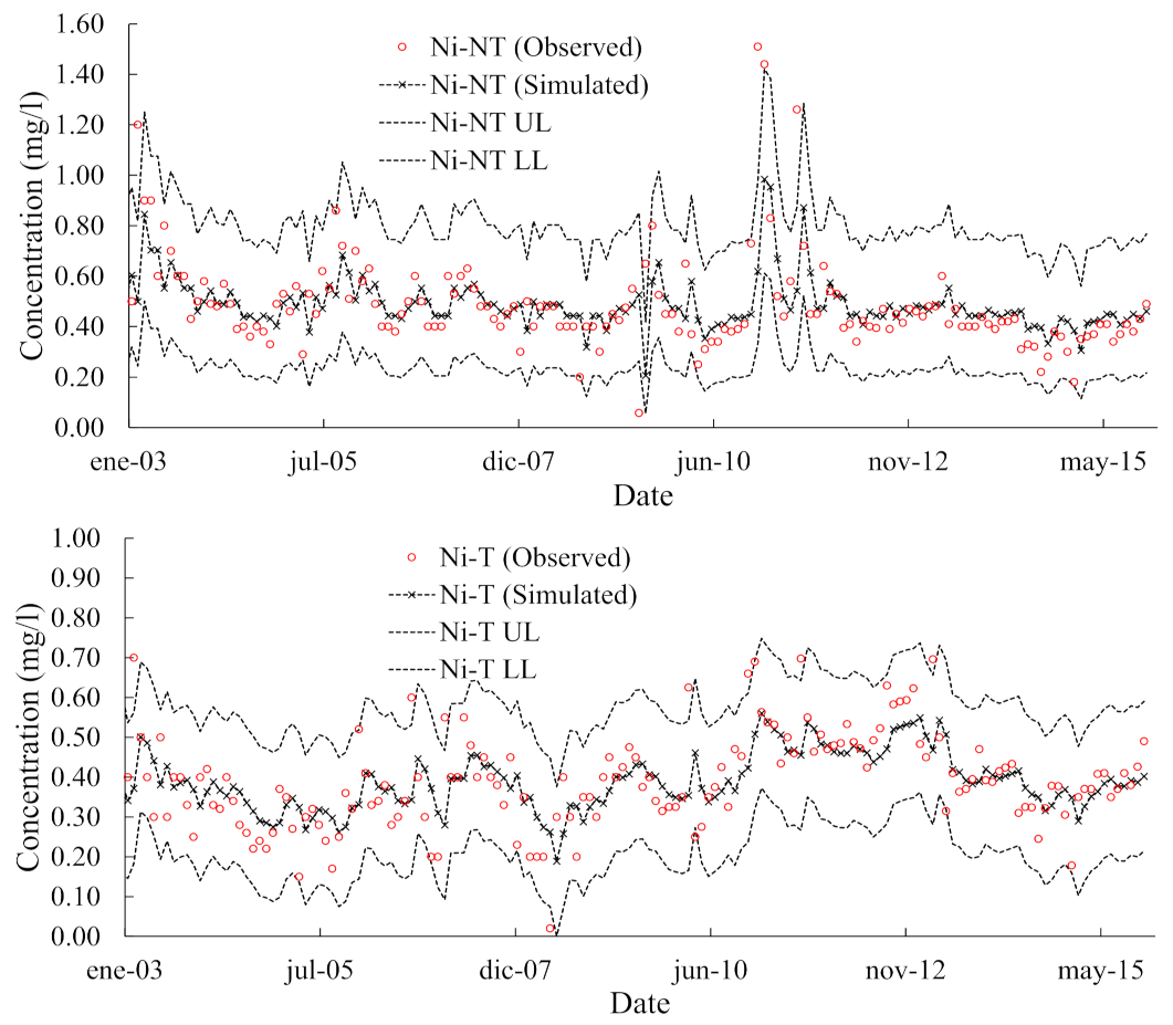
  • The ARIMA results confirm that the concentrations of HMs, BOD5, and COD in untreated leachate do not follow the same annual cycles observed for the MSW quantity disposed in the landfill. This difference is possibly associated with the leachate HRT in the conduction and pre-treatment system. ARIMA analysis suggests an HRT of up to one month (AR = 1) for HMs identified as indicators of untreated leachate (Cu, Pb, and Zn). As expected, there is also no seasonal component for ARIMA models of the HMs identified as indicators of treated leachate (Fe and Ni). Therefore, there is no transfer in time of the effect, which allows scheduling the operation of the treatment system under study;
  • The findings suggest that Cd is the HM with the largest concentration variations in untreated leachate during the study period (MA = 11). This HM shows variations over periods of 11 consecutive months. Differences in the MA term of the developed models suggest that Cd and Co are the most difficult HMs to homogenize in pre-treatment ponds;
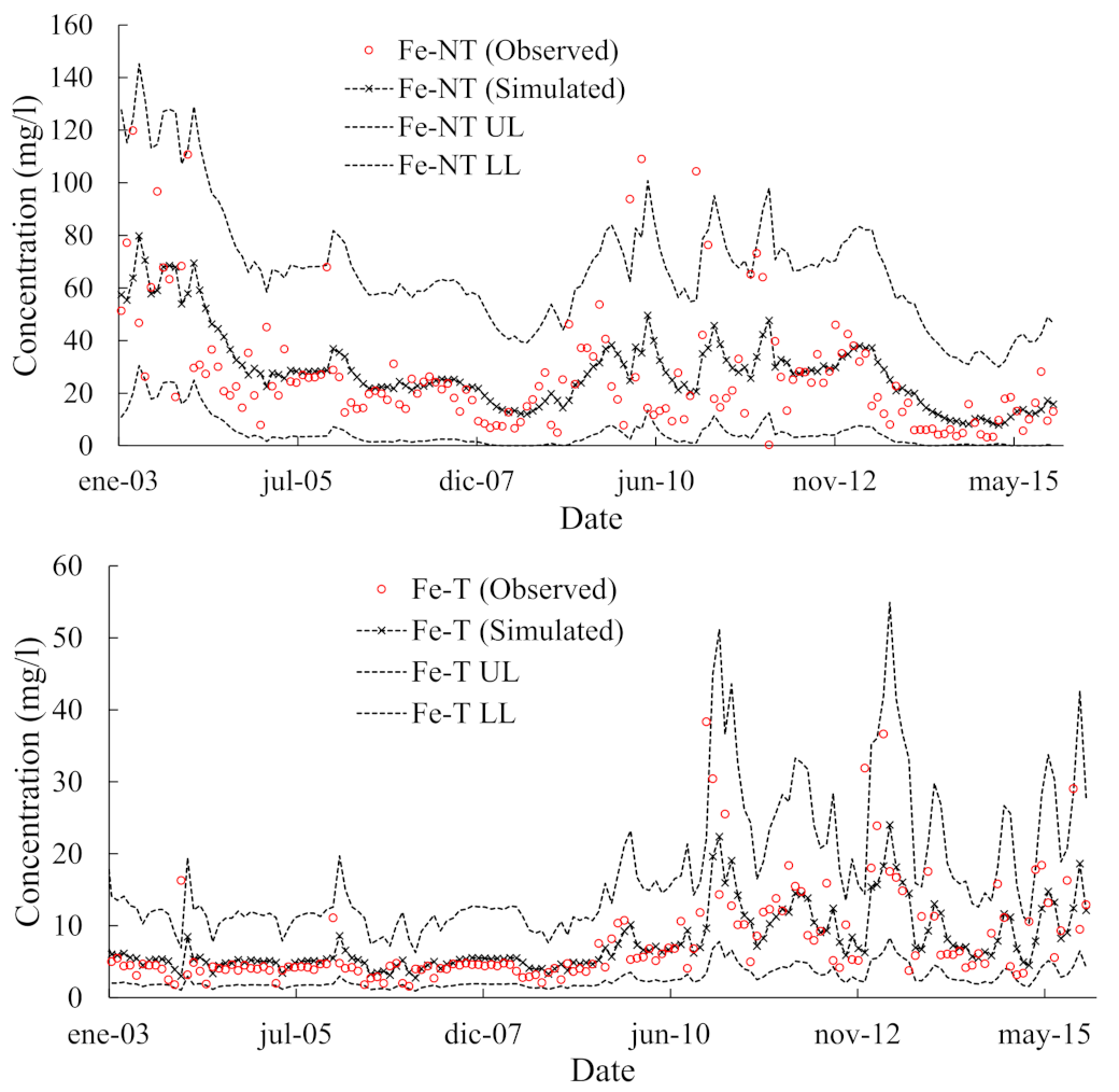
  • The removal efficiency of indicator HMs of the treatment plant operation (Fe and Ni) is probably conditioned by processes carried out over a period of one month (AR = 1). The high input concentration of these indicator HMs may prevent changing their ARIMA temporal structure during leachate treatment. This is reflected in the low removal efficiencies for all HMs under study (average = 26.1%);
  • The results show that during the treatment plant operation it is more difficult to control fluctuations in COD and BOD5 concentration (MA between 2–4), compared to fluctuations in HM concentration (MA between 0–2);
  • Finally, this study will be useful for deepening knowledge regarding the use of statistical models during the operation of leachate treatment systems in developing countries. This research will also be relevant for the public and private companies responsible for optimally scheduling the operation of these treatment systems.

Supplementary Materials

The following are available online at https://0-www-mdpi-com.brum.beds.ac.uk/article/10.3390/app11156988/s1, Figure S1: Scatter plots for the observed and simulated (ARIMA) values of Fe and Ni concentrations in untreated and treated leachate during the study period, Table S1: Pearson’s correlations between chemical characteristics of untreated leachate during the study period, Table S2: Parameter estimates for the ARIMA model terms selected for the variables considered in the untreated leachate, Table S3: Pearson’s correlations between chemical characteristics of treated leachate during the study period, Table S4: Parameter estimates for the ARIMA model terms selected for the variables considered in the treated leachate.

Author Contributions

Conceptualization, H.A.R.-Q., C.A.Z.-M., and D.A.Z.-A.; methodology, H.A.R.-Q. and C.A.Z.-M.; validation and formal analysis, D.A.Z.-A., H.A.R.-Q. and C.A.Z.-M.; resources, D.A.Z.-A., H.A.R.-Q., and C.A.Z.-M.; writing—original draft preparation, H.A.R.-Q. and C.A.Z.-M.; writing—review and editing, D.A.Z.-A. and H.A.R.-Q.; funding acquisition, D.A.Z.-A. All authors have read and agreed to the published version of the manuscript.

Funding

This research was funded by Centro de Investigaciones-Escuela de Ingenieros Militares (ESING), budget item A-02-02-02-008-001, Ejército Nacional de Colombia.

Institutional Review Board Statement

Not applicable.

Informed Consent Statement

Not applicable.

Data Availability Statement

Not applicable.

Conflicts of Interest

The authors declare no conflict of interest. The funders had no role in the design of the study; in the collection, analyses, or interpretation of data; in the writing of the manuscript; or in the decision to publish the results.

Abbreviations

ARAuto-regressive.
ARIMAAuto-regressive integrated moving average.
BICBayesian Information Criterion.
BOD5Biological oxygen demand.
CODChemical oxygen demand.
HMHeavy metal.
HRTHydraulic retention time.
LTSLeachate treatment systems.
MAMoving average.
MAEMean absolute error.
MAPEMean absolute percentage error.
MSWMunicipal solid waste.
Q’Ljung–Box statistic.
R2Coefficient of determination.
RMSERoot mean square error.
TSSTotal suspended solids.
WTPWastewater treatment plant.

References

  1. Propp, V.R.; De Silva, A.O.; Spencer, C.; Brown, S.J.; Catingan, S.D.; Smith, J.E.; Roy, J.W. Organic contaminants of emerging concern in leachate of historic municipal landfills. Environ. Pollut. 2021, 276, 116474. [Google Scholar] [CrossRef]
  2. Mishra, H.; Rathod, M.; Karmakar, S.; Kumar, R. A framework for assessment and characterisation of municipal solid waste landfill leachate: An application to the Turbhe landfill, Navi Mumbai, India. Environ. Monit. Assess. 2016, 188, 1–23. [Google Scholar] [CrossRef]
  3. Sauve, G.; Van Acker, K. The environmental impacts of municipal solid waste landfills in Europe: A life cycle assessment of proper reference cases to support decision making. J. Environ. Manag. 2020, 261, 110216. [Google Scholar] [CrossRef]
  4. Vaccari, M.; Tudor, T.; Vinti, G. Characteristics of leachate from landfills and dumpsites in Asia, Africa and Latin America: An overview. Waste Manag. 2019, 95, 416–431. [Google Scholar] [CrossRef] [PubMed]
  5. Righetto, I.; Al-Juboori, R.A.; Kaljunen, J.U.; Mikola, A. Multipurpose treatment of landfill leachate using natural coagulants—Pretreatment for nutrient recovery and removal of heavy metals and micropollutants. J. Environ. Chem. Eng. 2021, 9, 105213. [Google Scholar] [CrossRef]
  6. Min, J.-E.; Kim, M.; Kim, J.Y.; Park, I.-S.; Park, J.-W. Leachate modeling for a municipal solid waste landfill for upper expansion. KSCE J. Civ. Eng. 2010, 14, 473–480. [Google Scholar] [CrossRef]
  7. Wu, C.; Chen, W.; Gu, Z.; Li, Q. A review of the characteristics of Fenton and ozonation systems in landfill leachate treatment. Sci. Total Environ. 2021, 762, 143131. [Google Scholar] [CrossRef]
  8. González-Cortés, J.J.; Almenglo, F.; Ramírez, M.; Cantero, D. Effect of two different intermediate landfill leachates on the ammonium oxidation rate of non-adapted and adapted nitrifying biomass. J. Environ. Manag. 2021, 281, 111902. [Google Scholar] [CrossRef] [PubMed]
  9. Margallo, M.; Ziegler-Rodriguez, K.; Vázquez-Rowe, I.; Aldaco, R.; Irabien, Á.; Kahhat, R. Enhancing waste management strategies in Latin America under a holistic environmental assessment perspective: A review for policy support. Sci. Total Environ. 2019, 689, 1255–1275. [Google Scholar] [CrossRef]
  10. Rajoo, K.S.; Karam, D.S.; Ismail, A.; Arifin, A. Evaluating the leachate contamination impact of landfills and open dumpsites from developing countries using the proposed Leachate Pollution Index for Developing Countries (LPIDC). Environ. Nanotechnol. Monit. Manag. 2020, 14, 100372. [Google Scholar] [CrossRef]
  11. Manaf, L.A.; Samah, M.A.A.; Zukki, N.I.M. Municipal solid waste management in Malaysia: Practices and challenges. Waste Manag. 2009, 29, 2902–2906. [Google Scholar] [CrossRef]
  12. Kjeldsen, P.; Barlaz, M.A.; Rooker, A.P.; Baun, A.; Ledin, A.; Christensen, T.H. Present and Long-Term Composition of MSW Landfill Leachate: A Review. Crit. Rev. Environ. Sci. Technol. 2002, 32, 297–336. [Google Scholar] [CrossRef]
  13. Wijekoon, W.M.P.C.; Koliyabandara, P.A.; Cooray, A.; Lam, S.S.; Athapattu, B.C.L.; Vithanage, M. Progress and Prospects in Mitigation of Landfill Leachate Pollution: Risk, Pollution Potential, Treatment and Challenges. J. Hazard. Mater. 2021, 126627. [Google Scholar] [CrossRef]
  14. Luo, H.; Zeng, Y.; Cheng, Y.; He, D.; Pan, X. Recent advances in municipal landfill leachate: A review focusing on its characteristics, treatment, and toxicity assessment. Sci. Total Environ. 2020, 703, 135468. [Google Scholar] [CrossRef] [PubMed]
  15. Box, G.E.P.; Jenkins, G.M.; Reinsel, G.C.; Ljung, G.M. Time Series Analysis: Forecasting and Control; John Wiley & Sons: Hoboken, NJ, USA, 2015. [Google Scholar]
  16. Nourani, V.; Asghari, P.; Sharghi, E. Artificial intelligence based ensemble modeling of wastewater treatment plant using jittered data. J. Clean. Prod. 2021, 291, 125772. [Google Scholar] [CrossRef]
  17. Siddiqui, S.; Conkle, J.L.; Scarpa, J.; Sadovski, A. An analysis of U.S. wastewater treatment plant effluent dilution ratio: Implications for water quality and aquaculture. Sci. Total Environ. 2020, 721, 137819. [Google Scholar] [CrossRef]
  18. Dellana, S.A.; West, D. Predictive modeling for wastewater applications: Linear and nonlinear approaches. Environ. Model. Softw. 2009, 24, 96–106. [Google Scholar] [CrossRef]
  19. Chen, Z.; Min, H.; Hu, D.; Wang, H.; Zhao, Y.; Cui, Y.; Zou, X.; Wu, P.; Ge, H.; Luo, K.; et al. Performance of a novel multiple draft tubes airlift loop membrane bioreactor to treat ampicillin pharmaceutical wastewater under different temperatures. Chem. Eng. J. 2020, 380, 122521. [Google Scholar] [CrossRef]
  20. Selvaraj, J.J.; Arunachalam, V.; Coronado-Franco, K.V.; Romero-Orjuela, L.V.; Ramírez-Yara, Y.N. Time-series modeling of fishery landings in the Colombian Pacific Ocean using an ARIMA model. Reg. Stud. Mar. Sci. 2020, 39, 101477. [Google Scholar] [CrossRef]
  21. Jamil, R. Hydroelectricity consumption forecast for Pakistan using ARIMA modeling and supply-demand analysis for the year 2030. Renew. Energy 2020, 154, 1–10. [Google Scholar] [CrossRef]
  22. Zhang, F.; Yang, C.; Zhu, H.; Li, Y.; Gui, W. An integrated prediction model of heavy metal ion concentration for iron electrocoagulation process. Chem. Eng. J. 2020, 391, 123628. [Google Scholar] [CrossRef]
  23. Khashei, M.; Bijari, M. An artificial neural network (p,d,q) model for timeseries forecasting. Expert Syst. Appl. 2010, 37, 479–489. [Google Scholar] [CrossRef]
  24. Ebtehaj, I.; Bonakdari, H.; Zeynoddin, M.; Gharabaghi, B.; Azari, A. Evaluation of preprocessing techniques for improving the accuracy of stochastic rainfall forecast models. Int. J. Environ. Sci. Technol. 2020, 17, 505–524. [Google Scholar] [CrossRef]
  25. Maleki, A.; Nasseri, S.; Aminabad, M.S.; Hadi, M. Comparison of ARIMA and NNAR Models for Forecasting Water Treatment Plant’s Influent Characteristics. KSCE J. Civ. Eng. 2018, 22, 3233–3245. [Google Scholar] [CrossRef]
  26. Lotfi, K.; Bonakdari, H.; Ebtehaj, I.; Mjalli, F.S.; Zeynoddin, M.; Delatolla, R.; Gharabaghi, B. Predicting wastewater treatment plant quality parameters using a novel hybrid linear-nonlinear methodology. J. Environ. Manag. 2019, 240, 463–474. [Google Scholar] [CrossRef]
  27. Ömer Faruk, D. A hybrid neural network and ARIMA model for water quality time series prediction. Eng. Appl. Artif. Intell. 2010, 23, 586–594. [Google Scholar] [CrossRef]
  28. Parmar, K.S.; Bhardwaj, R. Statistical, time series, and fractal analysis of full stretch of river Yamuna (India) for water quality management. Environ. Sci. Pollut. Res. Int. 2015, 22, 397–414. [Google Scholar] [CrossRef]
  29. Ahmad, S.; Khan, I.H.; Parida, B.P. Performance of stochastic approaches for forecasting river water quality. Water Res. 2001, 35, 4261–4266. [Google Scholar] [CrossRef]
  30. Taheri Tizro, A.; Ghashghaie, M.; Georgiou, P.; Voudouris, K. Time series analysis of water quality parameters. J. Appl. Res. Water Wastewater 2014, 1, 40–50. [Google Scholar]
  31. Baird, R.B.; Eaton, A.D.; Rice editors, E.W. Standard Methods for the Examination of Water and Wastewater, 23rd ed.; American Public Health Association (APHA); American Water Works Association (AWWA); Water Environment Federation (WEF): Washington, DC, USA, 2017. [Google Scholar]
  32. MADS. Resolución 631 de 2015 Ministerio de Ambiente y Desarrollo Sostenible. 2015. Available online: https://www.alcaldiabogota.gov.co/sisjur/normas/Norma1.jsp?i=70346 (accessed on 30 September 2020).
  33. BOE. Real Decreto 646/2020. Available online: https://www.boe.es/buscar/act.php?id=BOE-A-2020-7438 (accessed on 1 March 2020).
  34. Romero-Aguilar, M.; Colín-Cruz, A.; Sánchez-Salinas, E.; Ortiz-Hernández, M.L. Wastewater treatment by an artificial wetlands pilot system: Evaluation of the organic charge removal. Rev. Int. Contam. Ambient. 2009, 25, 157–167. [Google Scholar]
  35. Guerrero-Guzmán, V.-M. Análisis Estadístico de Series de Tiempo Económicas; International Thomson: México City, Mexico, 2003. [Google Scholar]
  36. IBM. Time Series Modeler. 2021. Available online: https://prod.ibmdocs-production-dal-6099123ce774e592a519d7c33db8265e-0000.us-south.containers.appdomain.cloud/docs/ko/spss-statistics/24.0.0?topic=option-time-series-modeler (accessed on 28 June 2021).
  37. Ljung, G.M.; Box, G.E.P. On a Measure of Lack of Fit in Time Series Models. Biometrika 1978, 65, 297–303. [Google Scholar] [CrossRef]
  38. Schwarz, G. Estimating the Dimension of a Model. Ann. Stat. 1978, 6, 461–464. [Google Scholar] [CrossRef]
  39. Kumar, U.; Jain, V.K. ARIMA forecasting of ambient air pollutants (O3, NO, NO2 and CO). Stoch. Environ. Res. Risk Assess. 2010, 24, 751–760. [Google Scholar] [CrossRef]
  40. Zafra-Mejía, C.; Romero-Torres, D. Tendencias tecnológicas de depuración de lixiviados en rellenos sanitarios iberoamericanos. Rev. Ing. Univ. De Medellín 2019, 18, 125–147. [Google Scholar] [CrossRef]
  41. Ehrig, H.-J.; Stegmann, R. Chapter 10.2—Leachate Quality. In Solid Waste Landfilling; Cossu, R., Stegmann, R., Eds.; Elsevier: Amsterdam, The Netherlands, 2018; pp. 511–539. [Google Scholar]
  42. Raghab, S.M.; Abd El Meguid, A.M.; Hegazi, H.A. Treatment of leachate from municipal solid waste landfill. HBRC J. 2013, 9, 187–192. [Google Scholar] [CrossRef] [Green Version]
  43. Lozano-Rivas, W.A. Uso del extracto de fique (Furcraea sp.) como coadyuvante de coagulación en tratamiento de lixiviados. Rev. Int. Contam. Ambient. 2012, 28, 219–227. Available online: http://www.scielo.org.mx/scielo.php?script=sci_abstract&pid=S0188-49992012000300004&lng=es&nrm=iso&tlng=es (accessed on 1 March 2020).
  44. Novelo, R.I.M.; Reyes, R.B.G.; Borges, E.R.C.; Riancho, M.R.S. Treating leachate by Fenton oxidation. Ing. E Investig. 2010, 30, 80–85. [Google Scholar]
  45. Trujillo, D.; Font, X.; Sánchez, A. Use of Fenton reaction for the treatment of leachate from composting of different wastes. J. Hazard. Mater. 2006, 138, 201–204. [Google Scholar] [CrossRef] [PubMed] [Green Version]
  46. Reinhart, D.R.; Basel Al-Yousfi, A. The Impact of Leachate Recirculation on Municipal Solid Waste Landfill Operating Characteristics. Waste Manag. Res. 1996, 14, 337–346. [Google Scholar] [CrossRef]
  47. Heang, N.H.; Chiemchaisri, C.; Chiemchaisri, W.; Shoda, M. Treatment of municipal landfill leachate at different stabilization stages in two-stage membrane bioreactor bioaugmented with Alcaligenes faecalis no. 4. Bioresour. Technol. Rep. 2020, 11, 100528. [Google Scholar] [CrossRef]
  48. Renou, S.; Givaudan, J.G.; Poulain, S.; Dirassouyan, F.; Moulin, P. Landfill leachate treatment: Review and opportunity. J. Hazard. Mater. 2008, 150, 468–493. [Google Scholar] [CrossRef]
  49. De Castro, T.M.; Arantes, E.J.; de Mendonça Costa, M.S.S.; Gotardo, J.T.; Passig, F.H.; de Carvalho, K.Q.; Gomes, S.D. Anaerobic co-digestion of industrial waste landfill leachate and glycerin in a continuous anaerobic bioreactor with a fixed-structured bed (ABFSB): Effects of volumetric organic loading rate and alkaline supplementation. Renew. Energy 2021, 164, 1436–1446. [Google Scholar] [CrossRef]
  50. Wdowczyk, A.; Szymańska-Pulikowska, A. Differences in the Composition of Leachate from Active and Non-Operational Municipal Waste Landfills in Poland. Water 2020, 12, 3129. [Google Scholar] [CrossRef]
  51. Wiszniowski, J.; Robert, D.; Surmacz-Gorska, J.; Miksch, K.; Weber, J.V. Landfill leachate treatment methods: A review. Environ. Chem. Lett. 2006, 4, 51–61. [Google Scholar] [CrossRef]
  52. Youcai, Z. Chapter 5—Leachate Treatment Engineering Processes. In Pollution Control Technology for Leachate from Municipal Solid Waste; Youcai, Z., Ed.; Butterworth-Heinemann: Cambridge, MA, USA, 2018; pp. 361–522. [Google Scholar]
  53. Bolyard, S.C.; Reinhart, D.R. Application of landfill treatment approaches for stabilization of municipal solid waste. Waste Manag. 2016, 55, 22–30. [Google Scholar] [CrossRef] [PubMed] [Green Version]
  54. Al-Yaqout, A.F.; Hamoda, M.F. Evaluation of landfill leachate in arid climate—A case study. Environ. Int. 2003, 29, 593–600. [Google Scholar] [CrossRef]
  55. El-Gendy, A.S.; Biswas, N.; Bewtra, J.K. Municipal landfill leachate treatment for metal removal using water hyacinth in a floating aquatic system. Water Environ. Res. A Res. Publ. Water Environ. Fed. 2006, 78, 951–964. [Google Scholar] [CrossRef] [PubMed]
  56. Carvajal, E.; Cardona, S.-A. Technologies applicable to the removal of heavy metals from landfill leachate. Environ. Sci. Pollut. Res. 2019, 26, 15725–15753. [Google Scholar] [CrossRef] [PubMed]
Figure 1. Location of the study area: (a) MSW disposal area and (b) leachate treatment plant (Google Earth Pro, 2021).
Applsci 11 06988 g001
Figure 2. Pearson’s correlation matrix between chemical characteristics of untreated leachate during the study period.
Applsci 11 06988 g002
Figure 3. Principal component diagram for the concentrations of HMs, BOD5, and COD. (a) Untreated and (b) treated leachate.
Applsci 11 06988 g003
Figure 4. Pearson’s correlation matrix between chemical characteristics of treated leachate during the study period.
Applsci 11 06988 g004
Figure 5. Observed and simulated (ARIMA) values for Fe and Ni concentrations in untreated and treated leachate during the study period. NT = Untreated, T = Treated, UL = Upper limit, and LL = Lower limit.
Applsci 11 06988 g005aApplsci 11 06988 g005b
Table 1. Quantity of MSWs disposed, chemical characteristics of leachate, and removal efficiency from the treatment plant during the study period.
Untreated Leachate
MSWFlowBOD5CODNH4CdZnHg
µ179,76515.3803414,65727070.0140.7900.015
û182,15714.9768814,00327330.0100.5300.008
Mi139,7986.9132.8219819590.0030.1200.001
Ma217,38626.019,40232,35839670.2004.8300.500
SD161684.33540384452870.0210.6620.043
AsCuFePbCoCrNipH
µ0.0290.30397.20.2360.0960.7170.4888.29
û0.0200.09020.30.1900.0800.7000.4508.34
Mi0.0010.0100.2600.0100.0300.0200.0587.49
Ma0.11030.010,9008.2800.6803.0751.5109.38
SD0.0312.4138880.6580.0630.3580.1940.31
Treated Leachate
MSWFlowBOD5CODNH4CdZnHg
µ179,76515.150325214650.0110.4040.005
û182,15714.999.022812500.0100.3700.004
Mi139,7985.7114.025.031.00.0050.1000.001
Ma217,38625.5575011,07421520.0411.3600.029
SD16,1684.3686816015650.0080.2070.004
AsCuFePbCoCrNipH
µ0.0140.0807.780.1210.0600.4550.3908.19
û0.0100.0504.780.1000.0500.4000.3848.35
Mi0.0000.0101.600.0050.0200.0300.0207.00
Ma0.0650.20038.40.4170.1881.5000.7009.00
SD0.0140.0686.630.0660.0290.2370.1190.46
Removal (%)
MSWFlowBOD5CODNH4CdZnHg
µ--86.363.888.717.026.819.3
û--87.067.589.017.027.518.0
Mi--78.034.085.015.04.000.00
Ma--89.076.094.019.041.052.0
SD--3.1711.42.742.8311.114.8
AsCuFePbCoCrNipH
µ27.426.052.423.522.533.512.8-
û27.529.553.022.526.535.012.0-
Mi20.02.0042.012.08.0018.09.0-
Ma39.033.059.037.031.043.018.0-
SD5.218.545.2210.38.578.673.31-
Note: µ = Mean, û = Median, Mi = Minimum, Ma = Maximum, and SD = Standard deviation. MSW in Ton/month, Flow in L/s, HM concentration in mg/L, and BOD5 and COD concentration in mg/L.
Table 2. ARIMA models for the chemical parameters of untreated and treated leachate.
ModelT aR2RMSE bMAPE cMAE dLjung–Box (Q’)
p-Value
BIC e
Untreated leachate
BOD5(0,1,1)(0,0,0)NT0.863199322013690.29415.2
COD(0,1,1)(0,0,0)NT0.847330224.521830.09516.2
NH4(1,0,3)(1,0,1)NT0.3372375.55145.60.10211.1
Cd(1,0,11)(0,0,1)NL0.2450.01936.00.0060.064−7.80
Zn(1,1,1)(0,0,0)NL0.3710.52438.70.2880.052−1.22
Hg(0,0,1)(0,0,0)NL0.0310.0412490.0110.796−6.30
As(2,0,0)(0,0,0)NL0.2450.0263490.0170.667−7.16
Cu(0,1,1)(0,0,0)NL0.3472.4343.70.2240.9811.80
Fe(1,0,1)(0,0,0)NL0.20389616386.660.35813.6
Pb(1,0,1)(0,0,0)NL0.3340.66963.30.1250.795−0.708
Co(0,0,2)(0,0,0)NL0.1050.06231.00.0300.278−5.45
Cr(1,0,0)(0,0,0)SR0.2910.30395.50.1960.153−2.32
Ni(1,0,0)(0,0,0)SR0.3290.15924.10.0970.145−3.60
pH(1,0,0)(0,0,0)NT0.4450.2281.900.1580.291−2.88
Treated leachate
BOD5(0,0,4)(0,0,0)NL0.514613112296.20.05112.9
COD(1,0,2)(0,0,1)SR0.65495177.2452.40.74413.8
NH4(0,1,0)(0,0,0)NT0.66032287.6182.10.88111.6
Cd(1,1,0)(0,0,0)NL0.6900.00414.10.0020.326−10.8
Zn(0,0,2)(0,0,0)NL0.3890.17633.50.1190.163−3.37
Hg(0,1,1)(0,0,0)NL0.3340.00479.40.0020.790−11.0
As(0,1,1)(0,0,0)NL0.1470.0151680.0100.153−8.40
Cu(0,1,1)(0,0,0)NT0.9140.02028.20.0110.302−7.78
Fe(1,0,1)(0,0,0)NL0.3985.1742.33.0150.3653.38
Pb(0,1,1)(0,0,0)SR0.3780.05235.40.0280.959−5.87
Co(0,1,1)(1,0,1)NL0.5530.01918.90.0120.797−7.79
Cr(1,0,2)(0,0,0)NL0.3890.18734.10.1190.975−3.22
Ni(1,0,1)(0,0,0)NT0.3650.09527.10.0690.736−4.60
pH(1,0,0)(0,0,0)NT0.5560.3092.740.2210.879−2.28
Note: a T = Transformation, NT = No transformation, NL = Natural log, and SR = Square root; b RMSE = Root mean square error; c MAPE = Mean absolute percentage error; d MAE = Mean absolute error; and e BIC = Normalized Bayesian Information Criterion. A constant was not included in the ARIMA models when differentiation was applied.
Publisher’s Note: MDPI stays neutral with regard to jurisdictional claims in published maps and institutional affiliations.

