
SPARQL2Flink: Evaluation of SPARQL Queries on Apache Flink
by
 , , , and
Oscar Ceballos
1 ,
,
Carlos Alberto Ramírez Restrepo
2,
María Constanza Pabón
2,
Andres M. Castillo
1,* and
Oscar Corcho
3 1
Escuela de Ingeniería de Sistemas y Computación, Universidad del Valle, Ciudad Universitaria Meléndez Calle 13 No. 100-00, Cali 760032, Colombia
2
Departamento de Electrónica y Ciencias de la Computación, Pontificia Universidad Javeriana Cali, Calle 18 No. 118-250, Cali 760031, Colombia
3
Ontology Engineering Group, Universidad Politécnica de Madrid, Campus de Montegancedo, Boadilla del Monte, 28660 Madrid, Spain
*
Author to whom correspondence should be addressed.
Appl. Sci. 2021, 11(15), 7033; https://0-doi-org.brum.beds.ac.uk/10.3390/app11157033
Submission received: 1 June 2021
/
Revised: 9 July 2021
/
Accepted: 11 July 2021
/
Published: 30 July 2021
(This article belongs to the Special Issue Big Data Management and Analysis with Distributed or Cloud Computing)
Abstract
:Existing SPARQL query engines and triple stores are continuously improved to handle more massive datasets. Several approaches have been developed in this context proposing the storage and querying of RDF data in a distributed fashion, mainly using the MapReduce Programming Model and Hadoop-based ecosystems. New trends in Big Data technologies have also emerged (e.g., Apache Spark, Apache Flink); they use distributed in-memory processing and promise to deliver higher data processing performance. In this paper, we present a formal interpretation of some PACT transformations implemented in the Apache Flink DataSet API. We use this formalization to provide a mapping to translate a SPARQL query to a Flink program. The mapping was implemented in a prototype used to determine the correctness and performance of the solution. The source code of the project is available in Github under the MIT license.
1. Introduction
The amount and size of datasets represented in the Resource Description Framework (RDF) [1] language are increasing; this leads to challenging the limits of existing triple stores and SPARQL query evaluation technologies, requiring more efficient query evaluation techniques. Several proposals have been documented in state of the art use of Big Data technologies for storing and querying RDF data [2,3,4,5,6]. Some of these proposals have focused on executing SPARQL queries on the MapReduce Programming Model [7] and its implementation, Hadoop [8]. However, more recent Big Data technologies have emerged (e.g., Apache Spark [9], Apache Flink [10], Google DataFlow [11]). They use distributed in-memory processing and promise to deliver higher data processing performance than traditional MapReduce platforms [12]. These technologies are widely used in research projects and all kinds of companies (e.g., Google, Twitter, and Netflix, or even by small start-ups).
To analyze whether or not we can use these technologies to provide query evaluation over large RDF datasets, we will work with Apache Flink, an open-source platform for distributed stream and batch data processing. One of the essential components of the Flink framework is the Flink optimizer called Nephele [13]. Nephele is based on the Parallelization Contracts (PACTs) Programming Model [14] which is in turn a generalization of the well-known MapReduce Programming Model. The output of the Flink optimizer is a compiled and optimized PACT program which is a Directed Acyclic Graphs (DAG)-based dataflow program. At a high level, Flink programs are regular programs written in Java, Scala, or Python. Flink programs are mapped to dataflow programs, which implement multiple transformations (e.g., filter, map, join, group) on distributed collections, which are initially created from other sources (e.g., by reading from files). Results are returned via sinks, which may, for example, write the data to (distributed) files, or the standard output (e.g., to the command line terminal).
In [14], the set of initial PACTs operations (i.e., map, reduce, cross, cogroup, match) is formally described from the point of view of distributed data processing. Hence, the main challenge that we need to address is how to transform SPARQL queries into Flink programs that use the DataSet API’s Transformations? This paper presents an approach for SPARQL query evaluation over massive static RDF datasets through the Apache Flink framework. To summarize, the main contributions of this paper are the following:
- A formal definition of the Apache Flink’s subset transformations.
- A formal mapping to translate a SPARQL query to Flink program based on the DataSet API transformation.
- An open-source implementation, called SPARQL2Flink, available on Github under the MIT license, which transforms a SPARQL query into a Flink program. We assume that to deal with an RDF dataset encoding a SPARQL query is more accessible than writing a program using the Apache Flink DataSet API.
This research is a preliminary work towards making scalable queries processable in a framework like Apache Flink. We chose Apache Flink among several other Big Data tools based on comparative studies such as [12,15,16,17,18,19,20,21,22]. Flink provides a streaming data processing that incorporates (i) a distributed dataflow runtime that exploits pipelined streaming execution for batch and stream workloads, (ii) exactly-once state consistency through lightweight checkpointing, (iii) native iterative processing, and (iv) sophisticated window semantics, supporting out-of-order processing. The results reported in this paper focus on the processing of SPARQL queries over static RDF data through Apache Flink DataSet API. However, it is essential to note that this work is part of a general project that aims to process hybrid queries over massive static RDF data and append-only RDF streams. For example, the applications derived from the Internet of Things (IoT) that need to store, process, and analyze data in real or near real-time. In the Semantic Web context, so far, there have been some technologies trying to provide this capability [23,24,25,26]. Further work is needed to optimize the resulting Flink programs to ensure that queries can be run over large RDF datasets as described in our motivation.
The remainder of the paper is organized as follows: In Section 2, we present a brief overview of RDF, SPARQL, PACT Programming Model, and Apache Flink. In Section 3, we describe a formal interpretation of PACT transformations implemented in the Apache Flink DataSet API and the semantic correspondence between SPARQL Algebra operators and Apache Flink’s subset transformations. In Section 4, we present an implementation of the transformations described in Section 3, as a Java library. In Section 5, we present the evaluation of the performance of SPARQL2Flink using an adaptation of the Berlin SPARQL Benchmark [27]. In Section 6, we present related work on the SPARQL query processing of massive static RDF data which use MapReduce-based technologies. Finally, Section 7 presents conclusions and interesting issues for future work.
2. Background
2.1. Resource Description Framework
Resource Description Framework (RDF) [1] is a W3C recommendation for the representation of data on the Semantic Web. There are different serialization formats for RDF documents (e.g., RDF/XML, N-Triples, N3, Turtle). In the following, some essential elements of the RDF terminology are defined in an analogous way as Perez et al. do in [1,28].
Definition 1 (RDF Terms and Triples).
Assume there are pairwise disjoint infinite sets I, B, and L (IRIs, blank nodes, and literals). A tuple is called an RDF triple . In this tuple, s is called the subject, p the predicate, and o the object. We denote T (the set of RDF terms) as the union of IRIs, blank nodes, and literals, i.e., . IRI (Internationalized Resource Identifier) is a generalization of URI (Uniform Resource Identifier). URIs represent common global identifiers for resources across the Web.
Definition 2 (RDF Graph).
An RDF graph is a set of RDF triples. If G is an RDF graph, is the set of elements of appearing in the triples of G, and is the set of blank nodes appearing in G, i.e., .
Definition 3 (RDF Dataset).
An RDF dataset is a set where and are RDF graphs, and each corresponding is a distinct IRI. is called the default graph , while each of the others is called named graph.
2.2. SPARQL Protocol and RDF Query Language
SPARQL [29] is the W3C recommendation to query RDF. There are four query types: SELECT, ASK, DESCRIBE, and CONSTRUCT. In this paper, we focus on SELECT queries. The basic SELECT query consists of three parts separated by the keywords PREFIX, SELECT, and WHERE. The PREFIX part enables to declare prefixes to be used in IRIs to make them shorter; the SELECT part identifies the variables to appear in the query result; the WHERE part provides the Basic Graph Pattern (BGP) to match against the input data graph. A definition of terminology comprising the concepts of Triple and Basic Graph Pattern, Mappings, Basic Graph Patterns and Mappings, Subgraph Matching, Value Constraint, Built-in condition, Graph pattern expression, Graph Pattern Evaluation, and SELECT Result Form is done by Perez et al. in [28,30]. We encourage the reader to refer to these papers before going ahead.
2.3. PACT Programming Model
PACT Programming Model [14] is considered as a generalization of MapReduce [7]. The PACT Programming Model operates on a key/value data model and is based on so-called Parallelization Contracts (PACTs). A PACT consists of a system-provided second-order function (called Input Contract) and a user-defined first-order function (UDF) which processes custom data types. The PACT Programming Model provides an initial set of five Input Contracts that include two Single-Input Contracts: map and reduce as known from MapReduce which apply to user-defined functions with a single input, and three additional Multi-Input Contracts: cross, cogroup, and match which apply to user-defined functions for multiple inputs. As in the previous subsection, we encourage the reader to refer to the work of Battre at al. [14] for a complete review of the definitions concerning to the concepts of Simple-Input Contract, mapping function, map, reduce, Multi-Input Contract, cross, cogroup, and match.
2.4. Apache Flink
The Stratosphere [31] research project aims at building a big data analysis platform, which will make it possible to analyze massive amounts of data in a manageable and declarative way. In 2014 Stratosphere was open-sourced by the name Flink as an Apache Incubator project. It graduated to Apache Top Level project in the same year. Apache Flink [10] is an open-source framework for distributed stream and batch data processing. The main components of Apache Flink architecture are the core, the APIs (e.g., DataSet, DataStream, Table & SQL), and the libraries (e.g., Gelly). The core is a streaming dataflow engine that provides data distribution, communication, and fault tolerance, for distributed computations over data streams. The DataSet API allows processing finite datasets (batch processing), the DataStream API processes potentially unbounded data streams (stream processing), and the Table & SQL API allows the composition of queries from relational operators. The SQL support is based on Apache Calcite [32], which implements the SQL standard. The libraries are built upon those APIs. Apache Flink also provides an optimizer, called Nephele [13]. Nephele optimizer is based on the PACT Programming Model [14] and transforms a PACT program into a Job Graph [33]. Additionally, Apache Flink provides several PACT transformations for data transformation (e.g., filter, map, join, group).
3. Mapping SPARQL Queries to an Apache Flink Program
In this section, we present our first two contributions: the formal description of the Apache Flink’s subset transformations and the semantic correspondence between SPARQL Algebra operators and Apache Flink’s set transformations.
3.1. PACT Data Model
We describe the PACT Data Model in a way similar to the one in [34], which is centered around the concepts of datasets and records. We assume a possibly unbounded universal multi-set of records . In this way, a dataset is a bounded collection of records. Consequently, each dataset is a subset of the possibly unbounded universal multi-set , i.e., . A record is an unordered list of key-value pairs. The semantics of the keys and values, including their type is left to the user-defined functions that manipulate them [34]. We employ the record keys to define some PACT transformations. It is possible to use numbers as the record keys; in the special case where the keys of a record r is the set for some , we say r is a tuple. For the sake of simplicity, we write instead of tuple . Two records and are equal () iff and
3.2. Formalization of Apache Flink Transformations
In this section, we propose a formal interpretation of the PACT transformations implemented in the Apache Flink DataSet API. That interpretation will be used to establish a correspondence with the SPARQL Algebra operators. This correspondence is necessary before establishing an encoding to translate SPARQL queries to Flink programs in order to exploit the capabilities of Apache Flink for RDF data processing.
In order to define the PACT transformations, we need to define some auxiliary notions. First, we define the record projection, that builds a new record, which is made up of the key-value pairs associated with some specific keys. Second, we define the record value projection that allows obtaining the values associated with some specific keys. Next, we define the single dataset partition that creates groups of records where the values associated with some keys are the same. Finally, we define the multiple dataset partition as a generalization of the single dataset partition. The single dataset and the multiple dataset partitions are crucial to establish the definition of the reduce and the cogroup transformations due to the fact that they apply some specific user functions over groups of records.
Record projection is defined as follows:
Definition 4 (Record Projection).
Let be a record and be a set of keys, we define the projection of r over (denoted as ) as follows:
In this way, by means of a record projection, a new record is obtained only with the key-value pairs associated to some key in the set .
Record value projection is defined as follows:
Definition 5 (Record Value Projection).
Let be a record and be a tuple of keys such that , we define the value projection of r over (denoted as ) as follows:
where .
It is worth specifying that the record value projection takes a record and produces a tuple of values. In this way, in this operation, the key order in the tuple is considered for the result construction. Likewise, the result of the record value projection could contain repeated elements. Let and be tuples of values, we say that and are equivalent () if both and contain exactly the same elements.
The notion of single dataset partition as follows:
Definition 6 (Single Dataset Partition).
Let be a dataset and given a non-emtpy set of keys K, we define a single dataset partition of over keys K as:
where is a set partition of such that:
Intuitively, the single dataset partition creates groups of records where the values associated to some keys (set K) are the same.
Analogous to the single dataset partition, we define the multiple dataset partition below. It is possible to realize that the multiple dataset partition is a generalization of the single dataset partition.
Definition 7 (Multiple Dataset Partition).
Let be two datasets and given two non-emtpy set of keys and , we define a multiple dataset partition of and over keys as:
where is a set partition of such that:
After defining the auxiliary notions, we will define the map, reduce, filter, project, match, outer match, cogroup, and union PACT transformations.
Definition 8 (Map Transformation).
Let be a dataset and given a function f ranging over , i.e., , we define a map transformation as follows:
Correspondingly, the map transformation takes each record of a dataset and produces a new record by means of a user function f. Records produced by function f can differ with respect to the original records. First, the number of key-value pairs can be different, i.e., . Second, the keys do not have to match with the keys . Last, the datatype associated to each value can differ.
Accordingly, we define the reduce transformation as follows:
Definition 9 (Reduce Transformation).
Let be a dataset and given a non-emtpy set of keys K and a function f ranging over the power set of , i.e., , we define a reduce transformation as follows:
In this way, the reduce transformation takes a dataset and groups records by means of the single dataset partition. In each group, the records have the same values for the keys in set K. Then, it applies user function f over each group and produces a new record.
Definition 10 (Filter Transformation).
Let be a dataset and given a function f ranging over to boolean values, i.e., , we define a filter transformation as follows:
The filter transformation evaluates predicate f with every record of a dataset and it selects only those records with which f returns .
Definition 11 (Project Transformation).
Let be a dataset and given a set of keys , we define a project transformation as follows:
While filter transformation allows selecting some specific records according to some criteria, which are expressed in the semantics of a function f, the project transformation enables us to obtain some specific fields from the records of a dataset . For this purpose, we apply a record projection operation—to each record in with respect to a set of keys K. It is worth highlighting that the result of a project transformation is a multi-set due to several records having the same values in the keys of set K.
Previous PACT transformations take as a parameter a dataset and produce as a result a new dataset according to specific semantics. Nevertheless, a lot of data sources are available, and it is necessary to process and combine multiple datasets eventually. In consequence, some PACT transformations are taking two or more datasets as parameters [14]. Following, we present a formal interpretation of the essential multi-datasets transformations, including matching, grouping, and union.
Definition 12 (Match Transformation).
Let be datasets, given a function f ranging over and , i.e., and given sets of keys and , we define a match transformation as follows:
Thus, match transformation takes each pair of records built from datasets and , and applies user function f with those pairs for which the values in with respect to keys in coincide with the values in with respect to keys in . For this purpose, it checks this correspondence through a record value projection. Intuitively, the match transformation enables us to group and process pairs of records related to some specific criterion.
In some cases, it is necessary to match and process a record in a dataset even if a corresponding record does not exist in the other dataset. The outer match transformation extends the match transformation to enable such a matching. Outer match transformation is defined as follows:
Definition 13 (Outer Match Transformation).
Let be datasets, given a function f ranging over and , i.e., and given sets of keys and , we define a outer match transformation as follows:
In this manner, the outer match transformation is similar to the match transformation, but it allows us to apply the user function f with a record , although it does not exist a record that matches with record with respect to keys and .
In addition to the match and outer match transformations, the cogroup transformation enables us to group records in two datasets. Those records must coincide with respect to a set of keys. The cogroup transformation is defined as follows:
Definition 14 (CoGroup Transformation).
Let be datasets, given a function f ranging over and given sets of keys and , we define a cogroup transformation as follows:
Intuitively, cogroup transformation processes groups with the records on datasets and for which the values of the keys in and are equal. Then, it applies a user function f over each one of those groups.
Finally, the union transformation creates a new dataset with every record in two datasets and . It is defined as follows:
Definition 15 (Union Transformation).
Let be datasets, we define a union transformation as follows:
It is essential to highlight that records in dataset and can differ in the number of pairs key-value and the type of values.
3.3. Correspondence between SPARQL Algebra Operators and Apache Flink Transformations
In this section, we propose a semantic correspondence between SPARQL algebra operators and the PACT transformations implemented in the Apache Flink DataSet API. We use the formalization of PACT transformations presented in the previous section to provide an intuitive and correct mapping of the semantics elements of SPARQL queries. It is important to remember that in this formalization a record is an unordered list of n key-value pairs. However, as described in Section 2.1, an RDF dataset is a set of triples which is composed of three elements . Hence, for this particular case, a record will be understood as an unordered list of three key-value pairs. Besides, we assume that each field of a record r can be accessed using indexes 0, 1, and 2. Likewise, we assume that RDF triple pattern are triples where can be variables or values. Finally, the result of the application of each PACT transformation is intended to be a solution mapping, i.e., sets of key-value pairs with RDF variables as keys that will be represented as records with n key-value pairs.
Following, we present the definition of our encoding of SPARQL queries as PACT transformations. First, we define the encoding of the graph pattern evaluation as follows:
Definition 16 (Graph Pattern PACT Encoding).
Let P be a graph pattern and be an RDF dataset, the PACT encoding of the evaluation of P over , denoted by , is defined recursively as follows:
1. If P is a triple pattern then:
where function is defined as follows:
and function is defined as follows:
2. If P is then:
where and function is defined as follows:
3. If P is then:
where and function is defined as follows:
4. If P is then:
5. If P is then:
where function is defined as follows:
where R is a boolean expression and
In this way, the graph pattern PACT evaluation is encoded according to the recursive definition of a graph pattern P. More precisely, we have that:
- If P is a triple pattern, then records of dataset are filtered (by means of function ) to obtain only the records that are compatible with respect to the variables and values in . Then, the filtered records are mapped (by means function ) to obtain solution mappings that relate each variable to each possible value.
- If P is a join (left join) (it uses the SPARQL operators ()), then a () transformation is performed between the recursive evaluation of subgraphs and with respect to a set K conformed by the variables in and .
- If P is a union graph pattern, then there is a union transformation between the recursive evaluation of subgraphs and .
- Finally, if P is a filter graph pattern, then a transformation is performed over the recursive evaluation of subgraph where the user function f is built according to the structure of the filter expression R.
Additionally to the graph pattern evaluation, we present an encoding of the evaluation of SELECT and DISTINCT SELECT queries as well as the ORDER-BY and LIMIT modifiers. The selection encoding is defined as follows:
Definition 17 (Selection PACT Encoding).
Let be an RDF dataset, P be a graph pattern, K be a finite set of variables, and be a selection query over , the PACT Encoding of the evaluation of Q over is defined as follows:
Correspondingly, the selection query is encoded as a project transformation over the evaluation of the graph pattern P associated with the query with respect to a set of keys K conformed by the variables in the SELECT part of the query. We make a subtle variation in defining the distinct selection as follows:
Definition 18 (Distinct Selection PACT Encoding).
Let be an RDF dataset, P be a graph pattern, K be a finite set of variables, and be a distinct selection query over , the PACT Encoding of the evaluation of over is defined as follows:
where function is defined as follows:
The definition of the distinct selection PACT encoding is similar to the general selection query encoding. The main difference corresponds to a reduction step ( transformation) in which, the duplicate records, i.e., records with the same value in the keys of set K (the distinct keys) are reduced to only one occurrence by means of the function that takes as a parameter a set of records for which the value in the keys in K is the same and returns the first of them (actually, it could return any of them).
The encoding of the evaluation of a order-by query is defined as follows:
Definition 19 (Order By PACT Encoding).
Let be an RDF dataset, P be a graph pattern, k be a variable, and be an order by query over , the PACT Encoding of the evaluation of over is defined as follows:
where function is defined as follows:
where and is a permutation of M such that if or if , for each .
Thereby, the graph pattern associated with the query is first evaluated according to the encoding of its precise semantics. Then, the resulting solution mapping is ordered by means of a function . Currently, we only consider ordering with respect to one key, which is a simplification of the ORDER BY operator in SPARQL. Finally, the encoding of the evaluation of a limit query is defined as follows:
Definition 20 (Limit PACT Encoding).
Let be an RDF dataset, P be a graph pattern, m be an integer such that , and be a limit query over , the PACT Encoding of the evaluation of over is defined as follows:
where function is defined as follows:
where and such that , and .
In this way, once the graph pattern associated with the query is evaluated, the result is shortened to consider only the m records according to the query. According to the SPARQL semantics, if , the result is equal to M.
4. Implementation
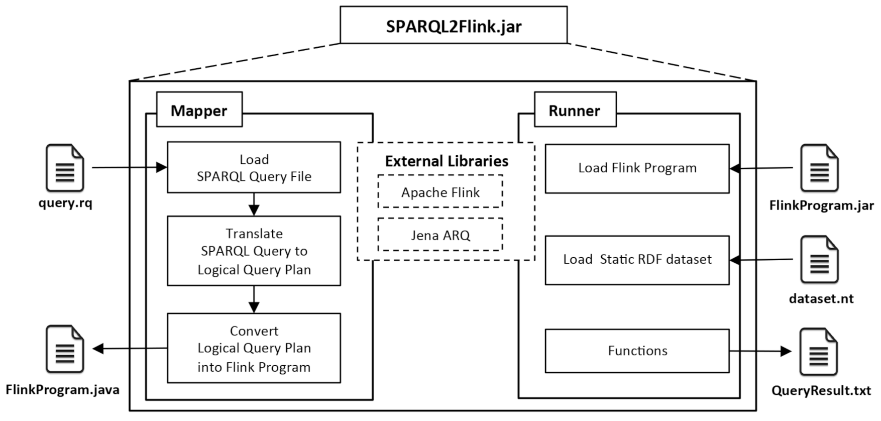
This section presents our last contribution. We implemented the transformations described in Section 3 as a Java library [35]. According to Apache Flink [10], a Flink program usually consists on four basic stages: (i) loading/creating the initial data, (ii) specifying the transformations of the data, (iii) specifying where to put the results of the computations, and (iv) triggering the program execution. The SPARQL2Flink [35] library—available on Github under the MIT license, is focused on the first three stages of a Flink program, and it is composed of two modules, called: Mapper and Runner, as shown in Figure 1. Apache Jena ARQ and Apache Flink libraries are shared among both modules.
The Mapper module transforms a declarative SPARQL query into an Apache Flink program (Flink program), and it is composed of three submodules:
Load SPARQL Query File: this submodule loads the declarative SPARQL query from a file with a .rq extension. Listing 1 shows an example of a SPARQL query that retrieves the names of all the people with their email if they have it.
| Listing 1. SPARQL query example. |
 |
Translate Query To a Logical Query Plan: this submodule uses the Jena ARQ library to translate the SPARQL query into a Logical Query Plan (LQP) expressed with SPARQL Algebra operators. The LQP is represented with an RDF-centric syntax provided by Jena, which is called SPARQL Syntax Expression (SSE) [36]. Listing 2 shows an LQP of the SPARQL query example.
| Listing 2. SPARQL Syntax Expression of the SPARQL query example. |
 |
Convert Logical Query Plan into Flink program: this submodule converts each SPARQL Algebra operator in the query to a transformation from the DataSet API of Apache Flink, according to the correspondence described in Section 3. For instance, each triple pattern within a Basic Graph Pattern (BGP) is encoded as a combination of filter and map transformations, the leftjoin operator is encoded as a leftOuterJoin transformation, whereas the project operator is expressed as a map transformation. Listing 3 shows the Java Flink program corresponding to the SPARQL query example.
| Listing 3. Java Flink program. |
 |
The Runner module allows executing a Flink program (as a jar file) on an Apache Flink stand-alone or local cluster mode. This module is composed of two submodules: Load RDF Dataset, which loads an RDF dataset in N-Triples format, and Functions, which contain several Java classes that allow us to solve the transformations within the Flink program.
5. Evaluation and Result
In this section, we present the evaluation of the performance of the SPARQL2Flink library by reusing a subset of the queries defined by the Berlin SPARQL Benchmark (BSBM) [27]. On the one hand, experiments were performed to empirically prove the correctness of the results of a SPARQL query transformed into a Flink program. On the other hand, experiments were carried out to show that our approach processes data that can scale as much as permitted by the underlying technology, in this case, Apache Flink. All experiments carried out in this section are available in [37].
The SPARQL2Flink library does not implement the SPARQL protocol and cannot be used as a SPARQL endpoint. It is important to note that this does not impose a strong limitation on our approach. This is an engineering task that will be supported in the future. For this reason, we do not use the test drive proposed in BSBM. Hence, we followed the following steps:
5.1. Generate Datasets from BSBM
BSBM is built around an e-commerce use case in which a set of products is offered by different vendors while consumers post reviews about the products [27]. Different datasets were generated using the BSBM data generator by setting up the number of products, number of producers, number of vendors, number of offers, and number of triples, as shown in Table 1.
For each dataset, one file was generated in N-Triples format. The name of each dataset is associated with the size of the dataset in gigabytes. The ds20mb dataset was used to perform the correctness tests. ds300mb, ds600mb, ds1gb, ds2gb, and ds18gb datasets were used to perform the scalability tests in the local cluster.
5.2. Verify Which SPARQL Query Templates Are Supported
The BSBM offers 12 different SPARQL query templates to emulate the search and navigation pattern of a consumer looking for a product [27]. We modified the query template omitting SPARQL operators and expressions that are not yet implemented in the library. The SPARQL query templates Q1, Q2, Q3, Q4, Q5, Q7, Q8, Q10, and Q11 were instantiated. Table 2 summarizes the list of queries that are Supported (S), Partially Supported (PS), and Not Supported (NS) by SPARQL2Flink library. In the case where the query is Partially Supported, it is detailed how the query was modified to be able to transform it into a Flink program. The SPARQL queries instantiated can be seen in [37].
5.3. Transform SPARQL Query into a Flink Program through SPARQL2Flink
First, SPARQL2Flink converts each SPARQL query (i.e., Q1, Q2, Q3, Q4, Q5, Q7, Q8, Q10, and Q11) into a Logical Query Plan expressed in terms of SPARQL Syntax Expression (SSE). Then, each Logical Query Plan was transformed into a Flink program (packaged in a .jar file) through the SPARQL2Flink [35]. The Logical Query Plans and the Flink Programs can be seen in [37].
5.4. Perform Results Correctness Tests on a Standalone Environment
The formal correctness tests are beyond the scope of this paper. However, empirical correctness tests were performed on the results of the nine queries that SPARQ2Flink supports and partially supports. The nine queries were executed independently in Apache Jena 3.6.0 and Apache Flink 1.10.0 without Hadoop using the ds20mb dataset. Both applications were set up on a laptop with Intel Core Duo i5 2.8 GHz, 8 GB RAM, 1 TB solid-state disk, and Mac Sierra operating system. In this test, we compared the results of running each SPARQL query on Apache Jena and each corresponding Flink program on Apache Flink. The results of each query were compared manually, checking if they were the same. In all cases, they were. All results can be seen in [37].
5.5. Carry out Scalability Tests on a Local Cluster Environment
The Apache Flink local cluster needs at least one Job Manager and one or more Task Managers. The Job Manager is the master that coordinates and manages the execution of the program; the Task Managers are the workers or slaves that execute parts of the parallel programs. The parallelism of task execution was determined by using the Task Slots available on each Task Manager. In order to carry out scalability tests, we setup an Apache Flink local cluster with one master node and fifteen slave nodes; each slave node with one Task Slot. Table 3 shows an specifications of each node.
The flink-conf.yaml file is part of the Job Manager and the Task Manager and contains all cluster configurations as a flat collection of YAML(YAML Ain’t Markup Language–https://yaml.org accessed on 23 March 2020) key-value pairs. Most of the configurations are the same for the Job Manager node and the Task Manager nodes. The parameters listed in Listing 4 were set up in order to carry out scalability tests. The parameters not listed were maintained with default values. A detailed description of each parameter can be see in [38].
Two scalability tests were conducted. In both tests, the primary measure evaluated is the query execution time of nine queries on different datasets and number of nodes in the cluster. Based on the number of available nodes, we configured five different clusters. C1 cluster with one master node and four slave nodes; C2 cluster with one master node and seven slave nodes; C3 cluster with one master node and eight slave nodes; C4 cluster with one master node and eleven slave nodes; C5 cluster with one master node and fifteen slave nodes.
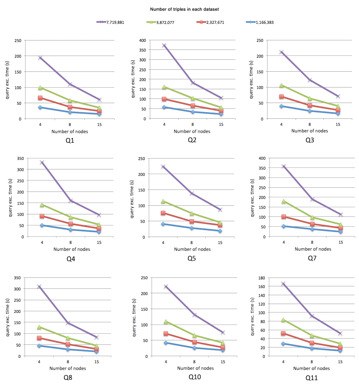
The first scalability test aims to evaluate the performance of SPARQL2Flink with ds300mb, ds600mb, ds1gb, and ds2gb datasets with a different number of triples. The test was performed on C1, C3, and C5 clusters. Each dataset was replicated on each node. Each node was configured with Apache Flink 1.10.0. A query executed on a dataset and a cluster configuration is considered an individual test. For instance, the query Q1 was executed on the ds300mb dataset on cluster C1. After that, the same query was executed on the same dataset on clusters C3 and C5. The remaining eight queries were executed on the other datasets and clusters in the same way. Consequently, a total of 108 tests were conducted. Figure 2 depicts the query execution times of nine queries after running the first scalability test.
| Listing 4. Apache Flink configuration: flink-conf.yml. |
 |
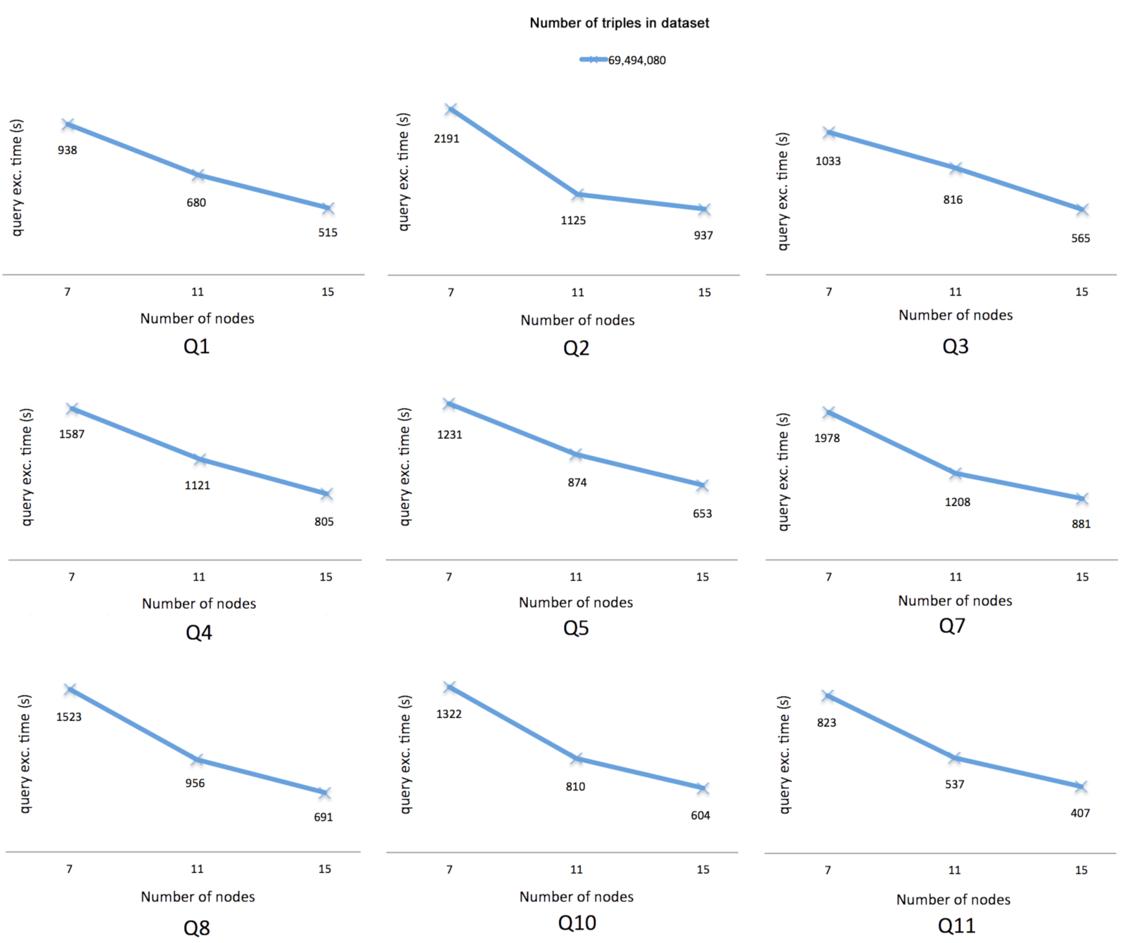
The second scalability test was performed on the C2, C4, and C5 clusters. For this test, Apache Flink 1.10.0 and Hadoop 2.8.3 were configured to use HDFS in order to store the ds18gb dataset. As in the first test, the nine queries were executed by changing the cluster configuration, for a total of 27 additional tests. Figure 3 depicts the query execution times of nine queries after running the second scalability test.
Each SPARQL query transformed into a Flink program generates a plan with several tasks. A task in Apache Flink is the basic unit of execution. It is the place where each parallel instance of an operator is executed. In terms of tasks, Q1 query generates 14 tasks, Q2 generates 31 tasks, Q3 generates 17 tasks, Q4 generates 28 tasks, Q5 generates 18 tasks, Q7 generates 29 tasks, Q8 generates 23 tasks, Q10 generates 18 tasks, and Q11 generates 6 tasks. All Flink program plans are available at [37]. In particular, the first task of the Flink program plan is associated with the dataset loading, the last task with the file creation which contains the query results, and the intermediate tasks are related to query execution. Table 4 describes the times of the dataset loading time, query execution time, and the sum of both.
6. Related Work
Several proposals have been documented in the use of Big Data technologies for storing and querying RDF data [2,3,4,5,6]. The most common way so far to query massive static RDF data has been rewriting SPARQL queries over the MapReduce Programming Model [7] and executing them on Hadoop [8] Ecosystems. A detailed comparison of existing approaches can be found in the survey presented in [3]. This work provides a comprehensive description of RDF data management in large-scale distributed platforms, where storage and query processing are performed in a distributed fashion, but under centralized control. The survey classifies the systems according to how they implement three fundamental functionalities: data storage, query processing, and reasoning; this determines how the triples are accessed and the number of MapReduce jobs. Additionally, it details the solutions adopted to implement those functionalities.
Another survey is [39], which presents a high-level overview of RDF data management, focusing on several approaches that have been adopted. The discussion focused on centralized RDF data management, distributed RDF systems, and querying over the Linked Open Data. In particular, in the distributed RDF systems, it identifies and discusses four classes of approaches: cloud-based solutions, partitioning-based approaches, federated SPARQL evaluation systems, and partial evaluation-based approach.
Given the success of NoSQL [40] (for “not only SQL”) systems, a number of authors have developed RDF data management systems based on these technologies. The survey in [41] provides a comprehensive study of the state of the art in data storage techniques, indexing strategies, and query execution mechanisms in the context of the RDF data processing. Part of this study summarizes the approaches that exploit NoSQL database systems for building scalable RDF management systems. In particular, [42] is recent example under NoSQL umbrella for efficiently evaluating SPARQL queries using MongoDB and Apache Spark. This work proposes an effective data model for storing RDF data in a document database, called node-oriented partition, using maximum replication factor of 2 (i.e., in the worst-case scenario, the data graph will be doubled in storage size). Each query is decomposed into a set of generalized star queries, which ensures that no joining operations over multiple datasets are required. The authors propose an efficient and simple distributed algorithm for partitioning large RDF data graphs based on the fact that each SPARQL query Q can be decomposed into a set of generalized star queries which can be evaluated independently of each other and can be used to compute the answers of the initial query Q [43].
In recent years, new trends in Big Data Technologies such as Apache Spark [9], Apache Flink [10], and Google DataFlow [11] have been proposed. They use distributed in-memory processing and promise to deliver higher performance data processing than traditional MapReduce platforms [12]. In particular, Apache Spark implements a programming model similar to MapReduce but extends it with two abstractions: Resilient Distributed Datasets (RDDs) [44] and Data Frames (DF) [45]. RDDs are a distributed, immutable, and fault-tolerant memory abstraction and DF is a compressed and schema-enabled data abstraction.
The survey [46] summarizes the approaches that use Apache Spark for querying large RDF data. For example, S2RDF [47] proposes a novel relational schema and relies on a translation of SPARQL queries into SQL for being executed using Spark SQL. The new relational partitioning schema for RDF data is called Extended Vertical Partitioning (ExtVP) [48]. In this schema, the RDF triples are distributed in pairs of columns, each one corresponding to an RDF term (the subject and the object). The relations are computed at the data load time using semi-joins, akin to the concept of Join Indices [49] in relational databases, to limit the number of comparisons when joining triple patterns. Each triple pattern of a query is translated into a single SQL query, and the query performance is optimized using the set of statistics and additional data structures computed during the data pre-processing step. The authors in [50] propose and compare five different query processing approaches based on different join execution models (i.e., partitioned join and broadcast join) on Spark components like RDD, DF, and SQL API. Morever, they propose a formalization for evaluating the cost of SPARQL query processing in a distributed setting. The main conclusion is that Spark SQL does not (yet) fully exploit the variety of distributed join algorithms and plans that could be executed using the Spark platform and propose some guidelines for more efficient implementations.
Google DataFlow [11] is a Programming Model and Cloud Service for batch and stream data processing with a unified API. It is built upon Google technologies, such as MapReduce for batch processing, FlumeJava [51] for programming model definition, and MillWheel [52] for stream processing. Google released the Dataflow Software Development Kit (SDK) as an open-source Apache project, named Apache Beam [53]. There are no works reported to the best of our knowledge that use Google Data-Flow to process massive static RDF datasets and RDF streams.
In a similar line to our approach, the authors in [54] propose FLINKer, which is a proposal to manage large RDF datasets and resolve SPARQL queries on top of Flink/Gelly. In practice, FLINKer makes use of Gelly to provide the vertex-centric view on graph processing, and the some DatasSet API operator to support each of the transformations required to resolve SPARQL queries. FLINKer uses the Jena ARQ SPARQL processor to parse a given SPARQL query and generate a parsing tree of operations, which are then resolved through the existing operators in the DataSet API of Flink, i.e., map, flatmap, filter, project, flatjoin, reducegroup, and iteration operators. The computation is performed through a sequence of iterations steps called supersteps. The main advantage of using Gelly as a backend is that Flink has native iterative support, i.e., the iterations do not require new job scheduling overheads to be performed.
The main difference between FLINKer and our proposal is the formalization of a set of PACT transformations implemented in the Apache Flink DataSet API and a formal mapping to translate a SPARQL query to a program based on the DataSet Flink program. We also provide an open-source implementation of our proposal as a Java library, available on Github under the MIT license. Besides, unlike FLINKer, we present an evaluation of the correctness and the performance of our tool by reusing a subset of the queries defined by the Berlin SPARQL Benchmark (BSBM). We did not find a FLINKer implementation available to perform a comparison against our proposal.
Table 5 summarizes a comparison of the main features of the approaches that use Apache Flink, like FLINKer and SPARQL2Flink, and Apache Spark in combinations with MongoDB.
7. Conclusions and Future Work
We have presented an approach for transforming SPARQL queries into Apache Flink programs for querying massive static RDF data. The main contributions of this paper are the formal definitions of the Apache Flink’s subset transformations, the definition of the semantic correspondence between Apache Flink’s subset transformations and the SPARQL Algebra operators, and the implementation of our approach as a library.
For the sake of simplicity, we limit to SELECT queries with SPARQL Algebra operators such as Basic Graph Pattern, AND (Join), OPTIONAL (LeftJoin), PROJECT, DISTINCT, ORDER BY, UNION, LIMIT, and specific FILTER expressions of the form (variable operator variable), (variable operator constant), and (constant operator variable). The operator within FILTER expression are logical connectives , inequality symbols , and equality symbol (=). Our approach does not support queries containing clauses or operators FROM, FROM NAMED, CONSTRUCT, DESCRIBE, ASK, INSERT, DELETE, LOAD, CLEAR, CREATE/DROP GRAPH, MINUS, or EXCEPT.
This work is the first step towards building up a Hybrid (batch and streaming) SPARQL query system on a Big Data scalable ecosystem. In this respect, the preliminary scalability tests with SPARQL2Flink show promising results in the processing of SPARQL queries over static RDF data. We can see that in all cases (i.e., Figure 2 and Figure 3), the query execution time decreases as the number of nodes in the cluster increases. However, improvements are still needed to optimize the processing of queries. It is important to note that our proposed approach and its implementation did not apply any optimization techniques. The generated Flink program process raw triples datasets.
The static RDF dataset used in our approach is serialized in a traditional plain format called N-Triples, which is the simplest form of the textual representation of RDF data but is also the most difficult to use because it does not allow URI abbreviation. The triples are given in subject, predicate, and object order as three complete URIs separated by spaces and encompassed by angle brackets (< and >). Each statement is given on a single line ended by a period (.). This approach results in a painful task requiring a great effort in terms of time and computational resources. Performance and scalability arise as significant issues in this scenario, and their resolution is closely related to the efficient storage and retrieval of the semantic data. Loading the raw triples to RAM significantly affects the dataset loading time (dlt), as can be seen in Table 4, more specifically, in the column labeled dlt. This value increases as the size of the dataset increases as well. For example, for the dataset with 69,494,080 triples, the loading time value is 938 s, using 4 nodes of the local cluster, when processing the Q1 query. This is because the SPARQL2Flink library does not yet implement optimization techniques. In future works, we will focus on two aspects: optimization techniques and RDF stream processing. We will study how to adapt some optimization techniques inherent in the processing of SPARQL queries like HDT compression [55,56,57] and multi-way join operators [58,59].
For RDF stream processing, we will extend the PACT Data Model to describe a formal interpretation of the data stream notion, the different window types, and the windowing operation necessary to establish an encoding to translate CQELS-QL [60] queries to DataStream PACT transformations. In practice, the DataStream API of the Apache Flink comes with predefined window assigners for the most common use cases, namely tumbling windows, sliding windows, session windows, and global windows. The window assigner defines how elements are assigned to windows. In particular, we focus on tumbling windows and sliding windows assigners in combination with time-based windows and count-based windows.
Author Contributions
Formalization, O.C. (Oscar Ceballos) and C.A.R.R.; methodology, O.C. (Oscar Ceballos), M.C.P. and A.M.C.; software, O.C. (Oscar Ceballos); validation, O.C. (Oscar Ceballos); investigation, O.C. (Oscar Ceballos); resources, O.C. (Oscar Ceballos); data curation, O.C. (Oscar Ceballos), M.C.P. and A.M.C.; writing—original draft preparation, O.C. (Oscar Ceballos); writing—review and editing, C.A.R.R., M.C.P., A.M.C., and O.C. (Oscar Corcho); supervision, M.C.P., A.M.C., and O.C. (Oscar Corcho); project administration, A.M.C.; funding acquisition, O.C. (Oscar Ceballos). All authors have read and agreed to the published version of the manuscript.
Funding
Oscar Ceballos is supported by the Colombian Administrative Department of Science, Technology and Innovation (Colciencias) [61] under the Ph.D. scholarship program 617-2013.
Institutional Review Board Statement
Not applicable.
Informed Consent Statement
Not applicable.
Data Availability Statement
Not applicable.
Acknowledgments
Conflicts of Interest
The authors declare no conflict of interest.
References
- Klyne, G.; Carroll, J. Resource Description Framework (RDF): Concepts and Abstract Syntax. W3C Recommendation, 2004. Available online: https://www.w3.org/TR/rdf-concepts/ (accessed on 21 November 2017).
- Choi, H.; Son, J.; Cho, Y.; Sung, M.K.; Chung, Y.D. SPIDER: A System for Scalable, Parallel/Distributed Evaluation of Large-scale RDF Data. In Proceedings of the 18th ACM Conference on Information and Knowledge Management, CIKM ’09, Hong Kong, China, 2–6 November 2009; ACM: New York, NY, USA, 2009; pp. 2087–2088. [Google Scholar] [CrossRef]
- Kaoudi, Z.; Manolescu, I. RDF in the Clouds: A Survey. VLDB J. 2015, 24, 67–91. [Google Scholar] [CrossRef]
- Peng, P.; Zou, L.; Özsu, M.T.; Chen, L.; Zhao, D. Processing SPARQL Queries over Distributed RDF Graphs. VLDB J. 2016, 25, 243–268. [Google Scholar] [CrossRef] [Green Version]
- Khodke, P.; Lawange, S.; Bhagat, A.; Dongre, K.; Ingole, C. Query Processing over Large RDF Using SPARQL in Big Data. In Proceedings of the Second International Conference on Information and Communication Technology for Competitive Strategies, ICTCS ’16, Udaipur, India, 4–5 March 2016; ACM: New York, NY, USA, 2016; pp. 66:1–66:6. [Google Scholar] [CrossRef]
- Hasan, A.; Hammoud, M.; Nouri, R.; Sakr, S. DREAM in Action: A Distributed and Adaptive RDF System on the Cloud. In Proceedings of the 25th International Conference Companion on World Wide Web, WWW ’16 Companion, Montréal, QC, Canada, 11–15 May 2016; International World Wide Web Conferences Steering Committee: Geneva, Switzerland, 2016; pp. 191–194. [Google Scholar] [CrossRef] [Green Version]
- Dean, J.; Ghemawat, S. MapReduce: Simplified Data Processing on Large Clusters. Commun. ACM 2008, 51, 107–113. [Google Scholar] [CrossRef]
- Apache-Hadoop. The Apache Hadoop. Apache Software Fundation, 2008. Available online: http://hadoop.apache.org (accessed on 21 November 2017).
- Zaharia, M.; Xin, R.S.; Wendell, P.; Das, T.; Armbrust, M.; Dave, A.; Meng, X.; Rosen, J.; Venkataraman, S.; Franklin, M.J.; et al. Apache Spark: A Unified Engine for Big Data Processing. Commun. ACM 2016, 59, 56–65. [Google Scholar] [CrossRef]
- Carbone, P.; Katsifodimos, A.; Ewen, S.; Markl, V.; Haridi, S.; Tzoumas, K. Apache Flink: Stream and Batch Processing in a Single Engine. IEEE Data Eng. Bull. 2015, 38, 28–38. [Google Scholar]
- Akidau, T.; Bradshaw, R.; Chambers, C.; Chernyak, S.; Fernández-Moctezuma, R.J.; Lax, R.; McVeety, S.; Mills, D.; Perry, F.; Schmidt, E.; et al. The Dataflow Model: A Practical Approach to Balancing Correctness, Latency, and Cost in Massive-scale, Unbounded, Out-of-order Data Processing. Proc. VLDB Endow. 2015, 8, 1792–1803. [Google Scholar] [CrossRef]
- Alexandrov, A.; Ewen, S.; Heimel, M.; Hueske, F.; Kao, O.; Markl, V.; Nijkamp, E.; Warneke, D. MapReduce and PACT-comparing data parallel programming models. In Datenbanksysteme für Business, Technologie und Web (BTW); Härder, T., Lehner, W., Mitschang, B., Schöning, H., Schwarz, H., Eds.; Gesellschaft für Informatik e.V.: Bonn, Germany, 2011; pp. 25–44. [Google Scholar]
- Warneke, D.; Kao, O. Nephele: Efficient Parallel Data Processing in the Cloud. In Proceedings of the 2Nd Workshop on Many-Task Computing on Grids and Supercomputers, MTAGS ’09, Portland, OR, USA, 16 November 2009; ACM: New York, NY, USA, 2009; pp. 8:1–8:10. [Google Scholar] [CrossRef]
- Battré, D.; Ewen, S.; Hueske, F.; Kao, O.; Markl, V.; Warneke, D. Nephele/PACTs: A Programming Model and Execution Framework for Web-scale Analytical Processing. In Proceedings of the 1st ACM Symposium on Cloud Computing, SoCC ’10, Indianapolis, IN, USA, 10–11 June 2010; ACM: New York, NY, USA, 2010; pp. 119–130. [Google Scholar] [CrossRef]
- Spangenberg, N.; Roth, M.; Franczyk, B. Evaluating New Approaches of Big Data Analytics Frameworks. In Business Information Systems; Abramowicz, W., Ed.; Springer International Publishing: Cham, Switzerland, 2015; pp. 28–37. [Google Scholar]
- Chintapalli, S.; Dagit, D.; Evans, B.; Farivar, R.; Graves, T.; Holderbaugh, M.; Liu, Z.; Nusbaum, K.; Patil, K.; Peng-Boyang, J.; et al. Benchmarking Streaming Computation Engines at Yahoo! 2015. Available online: https://yahooeng.tumblr.com/post/135321837876/benchmarking-streaming-computation-engines-at (accessed on 18 September 2019).
- Koch, J.; Staudt, C.; Vogel, M.; Meyerhenke, H. An empirical comparison of Big Graph frameworks in the context of network analysis. Soc. Netw. Anal. Min. 2016, 6, 1–20. [Google Scholar] [CrossRef] [Green Version]
- Veiga, J.; Expósito, R.R.; Pardo, X.C.; Taboada, G.; Touriño, J. Performance evaluation of big data frameworks for large-scale data analytics. In Proceedings of the 2016 IEEE International Conference on Big Data (Big Data), Washington, DC, USA, 5–8 December 2016; pp. 424–431. [Google Scholar]
- García-Gil, D.; Ramírez-Gallego, S.; García, S.; Herrera, F. A comparison on scalability for batch big data processing on Apache Spark and Apache Flink. Big Data Anal. 2017, 2, 1–11. [Google Scholar] [CrossRef] [Green Version]
- Morcos, M.; Lyu, B.; Kalathur, S. Solving the 2021 DEBS Grand Challenge Using Apache Flink. In Proceedings of the 15th ACM International Conference on Distributed and Event-Based Systems, Virtual Event, Italy, 28 June–2 July 2021; Association for Computing Machinery: New York, NY, USA, 2021; pp. 142–147. [Google Scholar] [CrossRef]
- Marić, J.; Pripužić, K.; Antonić, M. DEBS Grand Challenge: Real-Time Detection of Air Quality Improvement with Apache Flink. In Proceedings of the 15th ACM International Conference on Distributed and Event-Based Systems, Virtual Event, Italy, 28 June–2 July 2021; Association for Computing Machinery: New York, NY, USA, 2021; pp. 148–153. [Google Scholar] [CrossRef]
- Hesse, G.; Matthies, C.; Perscheid, M.; Uflacker, M.; Plattner, H. ESPBench: The Enterprise Stream Processing Benchmark. In Proceedings of the ACM/SPEC International Conference on Performance Engineering, Virtual Event, France, 19–23 April 2021; Association for Computing Machinery: New York, NY, USA, 2021; pp. 201–212. [Google Scholar] [CrossRef]
- Anicic, D.; Fodor, P.; Rudolph, S.; Stojanovic, N. EP-SPARQL: A Unified Language for Event Processing and Stream Reasoning. In Proceedings of the 20th International Conference on World Wide Web, Hyderabad, India, 28 March–1 April 2011; Association for Computing Machinery: New York, NY, USA, 2011; pp. 635–644. [Google Scholar] [CrossRef]
- Barbieri, D.F.; Braga, D.; Ceri, S.; Della Valle, E.; Grossniklaus, M. C-SPARQL: SPARQL for Continuous Querying. In Proceedings of the 18th International Conference on World Wide Web, Madrid, Spain, 20–24 April 2009; Association for Computing Machinery: New York, NY, USA, 2009; pp. 1061–1062. [Google Scholar] [CrossRef] [Green Version]
- Le-Phuoc, D.; Dao-Tran, M.; Parreira, J.X.; Hauswirth, M. A Native and Adaptive Approach for Unified Processing of Linked Streams and Linked Data. In Proceedings of the 10th International Conference on The Semantic Web—Volume Part I, Bonn, Germany, 23–27 October 2011; Springer: Berlin/Heidelberg, Germany, 2011; pp. 370–388. [Google Scholar]
- Le-Phuoc, D.; Nguyen Mau Quoc, H.; Le Van, C.; Hauswirth, M. Elastic and Scalable Processing of Linked Stream Data in the Cloud. In The Semantic Web—ISWC 2013; Alani, H., Kagal, L., Fokoue, A., Groth, P., Biemann, C., Parreira, J., Aroyo, L., Noy, N., Welty, C., Janowicz, K., Eds.; Lecture Notes in Computer Science; Springer: Berlin/Heidelberg, Germany, 2013; Volume 8218, pp. 280–297. [Google Scholar] [CrossRef] [Green Version]
- Bizer, C.; Schultz, A. The Berlin SPARQL Benchmark. Int. J. Semant. Web Inf. Syst. 2009, 5, 1–24. [Google Scholar] [CrossRef] [Green Version]
- Pérez, J.; Arenas, M.; Gutierrez, C. Semantics and Complexity of SPARQL. ACM Trans. Database Syst. 2009, 34, 16:1–16:45. [Google Scholar] [CrossRef] [Green Version]
- Prud’hommeaux, E.; Seaborne, A. SPARQL Query Language for RDF. W3C Recommendation, 2008. Available online: https://www.w3.org/TR/rdf-sparql-query/ (accessed on 21 November 2017).
- Pérez, J.; Arenas, M.; Gutierrez, C. Semantic of SPARQL; Technical Report TR/DCC-2006-17; Department of Computer Science, Universidad de Chile: Santiago de Chile, Chile, 2006. [Google Scholar]
- Alexandrov, A.; Bergmann, R.; Ewen, S.; Freytag, J.C.; Hueske, F.; Heise, A.; Kao, O.; Leich, M.; Leser, U.; Markl, V.; et al. The Stratosphere Platform for Big Data Analytics. VLDB J. 2014, 23, 939–964. [Google Scholar] [CrossRef]
- Apache-Calcite. The Apache Calcite. Apache Software Fundation, 2014. Available online: https://calcite.apache.org (accessed on 21 November 2017).
- Tzoumas, K.; Freytag, J.C.; Markl, V.; Hueske, F.; Peters, M.; Ringwald, M.; Krettek, A. Peeking into the Optimization of Data Flow Programs with MapReduce-style UDFs. In Proceedings of the 2013 IEEE International Conference on Data Engineering (ICDE 2013), Brisbane, Australia, 8–12 April 2013; IEEE Computer Society: Washington, DC, USA, 2013; pp. 1292–1295. [Google Scholar] [CrossRef] [Green Version]
- Hueske, F.; Peters, M.; Sax, M.J.; Rheinländer, A.; Bergmann, R.; Krettek, A.; Tzoumas, K. Opening the Black Boxes in Data Flow Optimization. Proc. VLDB Endow. 2012, 5, 1256–1267. [Google Scholar] [CrossRef]
- Ceballos, O. SPARQL2Flink Library. 2018. Available online: https://github.com/oscarceballos/sparql2flink (accessed on 24 March 2020).
- Apache-Jena. SPARQL Syntax Expression. Apache Software Fundation, 2011. Available online: https://jena.apache.org/documentation/notes/sse.html (accessed on 21 November 2017).
- Ceballos, O. SPARQL2Flink Test. 2019. Available online: https://github.com/oscarceballos/sparql2flink-test (accessed on 24 March 2020).
- Apache-Flink. Apache Flink Configuration. Apache Software Fundation, 2019. Available online: https://ci.apache.org/projects/flink/flink-docs-stable/ops/config.html (accessed on 14 May 2019).
- Özsu, M.T. A Survey of RDF Data Management Systems. Front. Comput. Sci. 2016, 10, 418–432. [Google Scholar] [CrossRef] [Green Version]
- Grolinger, K.; Higashino, W.A.; Tiwari, A.; Capretz, M.A. Data Management in Cloud Environments: NoSQL and NewSQL Data Stores. J. Cloud Comput. 2013, 2. [Google Scholar] [CrossRef] [Green Version]
- Wylot, M.; Hauswirth, M.; Cudré-Mauroux, P.; Sakr, S. RDF Data Storage and Query Processing Schemes: A Survey. ACM Comput. Surv. 2018, 51. [Google Scholar] [CrossRef]
- Kalogeros, E.; Damigos, M.; Gergatsoulis, M. Document-based RDF storage method for parallel evaluation of basic graph pattern queries. Int. J. Metadata Semant. Ontol. 2020, 14, 63. [Google Scholar] [CrossRef]
- Kalogeros, E.; Gergatsoulis, M.; Damigos, M. Redundancy in Linked Data Partitioning for Efficient Query Evaluation. In Proceedings of the 2015 3rd International Conference on Future Internet of Things and Cloud, Rome, Italy, 24–26 August 2015; pp. 497–504. [Google Scholar] [CrossRef]
- Zaharia, M.; Chowdhury, M.; Das, T.; Dave, A.; Ma, J.; McCauley, M.; Franklin, M.J.; Shenker, S.; Stoica, I. Resilient Distributed Datasets: A Fault-tolerant Abstraction for In-memory Cluster Computing. In Proceedings of the 9th USENIX Conference on Networked Systems Design and Implementation, San Jose, CA, USA, 25–27 April 2012; USENIX Association: Berkeley, CA, USA, 2012; p. 2. [Google Scholar]
- Armbrust, M.; Xin, R.S.; Lian, C.; Huai, Y.; Liu, D.; Bradley, J.K.; Meng, X.; Kaftan, T.; Franklin, M.J.; Ghodsi, A.; et al. Spark SQL: Relational Data Processing in Spark. In Proceedings of the 2015 ACM SIGMOD International Conference on Management of Data, Scottsdale, AZ, USA, 20–24 May 20215; ACM: New York, NY, USA, 2015; pp. 1383–1394. [Google Scholar] [CrossRef]
- Agathangelos, G.; Troullinou, G.; Kondylakis, H.; Stefanidis, K.; Plexousakis, D. RDF Query Answering Using Apache Spark: Review and Assessment. In Proceedings of the 2018 IEEE 34th International Conference on Data Engineering Workshops (ICDEW), Paris, France, 16–19 April 2018; pp. 54–59. [Google Scholar] [CrossRef] [Green Version]
- Schätzle, A.; Przyjaciel-Zablocki, M.; Skilevic, S.; Lausen, G. S2RDF: RDF Querying with SPARQL on Spark. Proc. VLDB Endow. 2016, 9, 804–815. [Google Scholar] [CrossRef]
- Abadi, D.J.; Marcus, A.; Madden, S.R.; Hollenbach, K. Scalable Semantic Web Data Management Using Vertical Partitioning. In Proceedings of the 33rd International Conference on Very Large Data Bases, VLDB Endowment, Vienna, Austria, 23–27 September 2007; pp. 411–422. [Google Scholar]
- Valduriez, P. Join Indices. ACM Trans. Database Syst. 1987, 12, 218–246. [Google Scholar] [CrossRef]
- Naacke, H.; Amann, B.; Curé, O. SPARQL Graph Pattern Processing with Apache Spark. In Proceedings of the Fifth International Workshop on Graph Data-management Experiences & Systems, Chicago, IL, USA, 14–19 May 2017; ACM: New York, NY, USA, 2017; pp. 1:1–1:7. [Google Scholar] [CrossRef]
- Chambers, C.; Raniwala, A.; Perry, F.; Adams, S.; Henry, R.R.; Bradshaw, R.; Weizenbaum, N. FlumeJava: Easy, Efficient Data-parallel Pipelines. SIGPLAN Not. 2010, 45, 363–375. [Google Scholar] [CrossRef]
- Akidau, T.; Balikov, A.; Bekiroğlu, K.; Chernyak, S.; Haberman, J.; Lax, R.; McVeety, S.; Mills, D.; Nordstrom, P.; Whittle, S. MillWheel: Fault-tolerant Stream Processing at Internet Scale. Proc. VLDB Endow. 2013, 6, 1033–1044. [Google Scholar] [CrossRef]
- Apache-Beam. The Apache Beam. Apache Software Fundation, 2017. Available online: https://beam.apache.org (accessed on 21 November 2017).
- Azzam, A.; Kirrane, S.; Polleres, A. Towards Making Distributed RDF Processing FLINKer. In Proceedings of the 2018 4th International Conference on Big Data Innovations and Applications (Innovate-Data), Barcelona, Spain, 6–8 August 2018; pp. 9–16. [Google Scholar] [CrossRef] [Green Version]
- Martínez-Prieto, M.A.; Fernández, J.D.; Cánovas, R. Querying RDF Dictionaries in Compressed Space. SIGAPP Appl. Comput. Rev. 2012, 12, 64–77. [Google Scholar] [CrossRef]
- Fernández, J.D. Binary RDF for Scalable Publishing, Exchanging and Consumption in the Web of Data. In Proceedings of the 21st International Conference on World Wide Web, Lyon, France, 16–20 April 2012; Association for Computing Machinery: New York, NY, USA, 2012; pp. 133–138. [Google Scholar] [CrossRef] [Green Version]
- Hernández-Illera, A.; Martínez-Prieto, M.A.; Fernández, J.D. Serializing RDF in Compressed Space. In Proceedings of the 2015 Data Compression Conference, Snowbird, UT, USA, 7–9 April 2015; pp. 363–372. [Google Scholar] [CrossRef]
- Afrati, F.N.; Ullman, J.D. Optimizing Joins in a Map-Reduce Environment. In Proceedings of the 13th International Conference on Extending Database Technology, Lausanne, Switzerland, 22–26 March 2010; Association for Computing Machinery: New York, NY, USA, 2010; pp. 99–110. [Google Scholar] [CrossRef] [Green Version]
- Galkin, M.; Endris, K.M.; Acosta, M.; Collarana, D.; Vidal, M.E.; Auer, S. SMJoin: A Multi-Way Join Operator for SPARQL Queries. In Proceedings of the 13th International Conference on Semantic Systems, Amsterdam, The Netherlands, 11–14 September 2017; Association for Computing Machinery: New York, NY, USA, 2017; pp. 104–111. [Google Scholar] [CrossRef]
- Calbimonte, J.P.; Corcho, O.; Gray, A.J.G. Enabling Ontology-Based Access to Streaming Data Sources. In Proceedings of the 9th International Semantic Web Conference on The Semantic Web—Volume Part I, Shanghai, China, 7–11 November 2010; Springer: Berlin/Heidelberg, Germany, 2010; pp. 96–111. [Google Scholar]
- Gobierno de Colombia. Colciencias. 2020. Available online: https://minciencias.gov.co/ (accessed on 24 March 2020).
- Gobierno de Colombia. Ministerio de Tecnologías de la Información y las Comunicaciones—MinTIC. 2020. Available online: https://www.mintic.gov.co/portal/inicio/ (accessed on 24 March 2020).
- Gobierno de Colombia. Gobernación de Nariño. 2020. Available online: https://narino.gov.co/ (accessed on 24 March 2020).
- Morán, G. ParqueSoft Nariño. 2020. Available online: https://www.parquesoftpasto.com/ (accessed on 24 March 2020).
Figure 1.
SPARQL2Flink conceptual architecture.

Figure 2.
Execution times of nine queries after running the first scalability test. The x-axis represents the number of nodes on cluster C1, C3, and C5. The y-axis represents the time in seconds, which includes the dataset loading time (dlt), the query execution time (qet), and the amount of time taken in creating the file with query results. Additionally, on the top, the number of triples of each dataset is shown.

Figure 3.
Execution times of nine queries after running the second scalability test. The x-axis represents the number of nodes on cluster C2, C4, and C5. The y-axis represents the time in seconds, which includes the dataset load time (dlt), the query execution time (qet), and the creation file time with query results. Additionally, on the top, the number of dataset triples is shown.


Table 1.
Datasets generated using the Berlin SPARQL Benchmark data generator.
| Dataset | Products | Producers | Vendors | Offers | No. Triples |
|---|---|---|---|---|---|
| ds20mb | 209 | 5 | 2 | 4180 | 78,351 |
| ds300mb | 3255 | 69 | 35 | 65,100 | 1,166,387 |
| ds600mb | 6521 | 135 | 63 | 130,620 | 2,327,671 |
| ds1gb | 10,519 | 225 | 108 | 219,400 | 3,872,077 |
| ds2gb | 219,00 | 443 | 223 | 43,800 | 7,719,881 |
| ds18gb | 47,884 | 3956 | 2027 | 4,000,000 | 69,494,080 |
Table 2.
BSBM SPARQL query templates Supported (S), Partially Supported (PS), and Not Supported (NS).
Table 2.
BSBM SPARQL query templates Supported (S), Partially Supported (PS), and Not Supported (NS).
| Query | Support | Reason | Modificaton |
|---|---|---|---|
| Q1 | S | - | - |
| Q2 | S | - | - |
| Q3 | PS | The bound function within the FILTER operator is not supported | The FILTER (!bound(?testVar)) expression is omitted |
| Q4 | PS | The OFFSET operator is not supported | The OFFSET 5 expression is omitted |
| Q5 | PS | The condition within the FILTER operator contains addition or subtraction operations which are not supported | The operations within the FILTER condition are changed by a constant in order to evaluate && operator |
| Q6 | PS | The regex function within the FILTER operator is not supported | The FILTER expression is omitted |
| Q7 | S | - | - |
| Q8 | PS | The langMatches and lang functions within the FILTER operator are not supported | The FILTER langMatches(lang(?text), "EN") expression is omitted |
| Q9 | NS | DESCRIBE query type is not supported | |
| Q10 | S | - | - |
| Q11 | S | - | - |
| Q12 | NS | CONSTRUCT query type is not supported | - |
Table 3.
Local cluster nodes specifications.
| Node | Specifications |
|---|---|
| master | Model: iMac13.2, SO: Sierra 10.12.1, Processor: Intel Quad Core i7 3.4 GHz, RAM: 32 GB, HD: 1 TB |
| slave01 to slave13 | Model: iMac13.2, SO: Mojave 10.14, Processor: Intel Quad Core i7 3.4 GHz, RAM: 32 GB, HD: 532 GB |
| slave14 | Model: iMac13.2, SO: Mojave 10.14, Processor: Intel Quad Core i5 2.9 GHz, RAM: 32 GB, HD: 532 GB |
| slave15 | Model: iMac13.2, SO: Mojave 10.14, Processor: Intel Quad Core i5 2.9 GHz, RAM: 16 GB, HD: 532 GB |
Table 4.
dlt+qet refers to the sum of dlt and qet times. dlt represents the dataset loading time which refers to the time spent to move each triple from a file into Apache Flink local cluster. qet represents the query execution time. The file creation time was ignored. In the worst case, it was less than or equal to 373 milliseconds. The times for query processing are in seconds.
| Dataset | 7,719,881 Triples | 3,872,077 Triples | 2,327,671 Triples | 1,166,387 Triples | 69,494,080 Triples | ||||||||||||
|---|---|---|---|---|---|---|---|---|---|---|---|---|---|---|---|---|---|
| Times | In Seconds | ||||||||||||||||
| Query | Nodes | dlt + qet | dlt | qet | dlt + qet | dlt | qet | dlt + qet | dlt | qet | dlt + qet | dlt | qet | Nodes | dlt + qet | dlt | qet |
| 4 | 194 | 166 | 28 | 100 | 85 | 15 | 67 | 56 | 11 | 36 | 30 | 6 | 7 | 938 | 816 | 122 | |
| Q1 | 8 | 110 | 95 | 28 | 58 | 49 | 9 | 37 | 31 | 6 | 21 | 16 | 5 | 11 | 680 | 535 | 145 |
| 15 | 61 | 52 | 9 | 35 | 29 | 6 | 24 | 19 | 5 | 15 | 12 | 3 | 15 | 515 | 403 | 112 | |
| 4 | 373 | 227 | 146 | 161 | 120 | 41 | 99 | 73 | 26 | 57 | 41 | 16 | 7 | 2191 | 1363 | 828 | |
| Q2 | 8 | 182 | 143 | 39 | 103 | 75 | 28 | 63 | 47 | 16 | 33 | 23 | 10 | 11 | 1125 | 770 | 355 |
| 15 | 105 | 78 | 27 | 56 | 42 | 14 | 39 | 27 | 12 | 22 | 16 | 6 | 15 | 937 | 586 | 351 | |
| 4 | 212 | 175 | 37 | 107 | 88 | 19 | 70 | 55 | 15 | 40 | 31 | 9 | 7 | 1033 | 842 | 191 | |
| Q3 | 8 | 123 | 103 | 20 | 64 | 52 | 12 | 42 | 33 | 9 | 24 | 18 | 6 | 11 | 816 | 584 | 232 |
| 15 | 71 | 57 | 14 | 40 | 31 | 9 | 27 | 20 | 7 | 16 | 12 | 4 | 15 | 565 | 421 | 144 | |
| 4 | 331 | 215 | 116 | 143 | 109 | 34 | 92 | 67 | 25 | 50 | 35 | 15 | 7 | 1587 | 1131 | 456 | |
| Q4 | 8 | 161 | 129 | 32 | 87 | 67 | 20 | 56 | 43 | 13 | 31 | 22 | 9 | 11 | 1121 | 717 | 404 |
| 15 | 97 | 75 | 22 | 53 | 38 | 15 | 36 | 25 | 11 | 21 | 15 | 6 | 15 | 805 | 536 | 269 | |
| 4 | 224 | 173 | 51 | 113 | 88 | 25 | 76 | 54 | 22 | 41 | 29 | 12 | 7 | 1231 | 867 | 364 | |
| Q5 | 8 | 138 | 100 | 38 | 75 | 53 | 22 | 49 | 33 | 16 | 28 | 18 | 10 | 11 | 874 | 584 | 290 |
| 15 | 87 | 57 | 30 | 46 | 31 | 15 | 37 | 20 | 17 | 19 | 13 | 6 | 15 | 653 | 421 | 232 | |
| 4 | 358 | 225 | 133 | 179 | 125 | 54 | 101 | 71 | 30 | 53 | 35 | 18 | 7 | 1978 | 1186 | 792 | |
| Q7 | 8 | 189 | 142 | 47 | 97 | 72 | 25 | 63 | 45 | 18 | 38 | 24 | 14 | 11 | 1208 | 741 | 467 |
| 15 | 112 | 77 | 35 | 61 | 39 | 22 | 42 | 27 | 15 | 24 | 15 | 9 | 15 | 881 | 553 | 328 | |
| 4 | 310 | 209 | 101 | 130 | 99 | 31 | 80 | 60 | 20 | 45 | 32 | 13 | 7 | 1523 | 988 | 535 | |
| Q8 | 8 | 147 | 117 | 30 | 80 | 60 | 20 | 52 | 38 | 14 | 29 | 21 | 8 | 11 | 956 | 645 | 311 |
| 15 | 84 | 65 | 19 | 46 | 34 | 12 | 31 | 22 | 9 | 20 | 14 | 6 | 15 | 691 | 476 | 215 | |
| 4 | 221 | 175 | 46 | 110 | 88 | 22 | 71 | 54 | 17 | 39 | 29 | 10 | 7 | 1322 | 884 | 438 | |
| Q10 | 8 | 131 | 103 | 28 | 66 | 51 | 15 | 44 | 33 | 11 | 26 | 18 | 8 | 11 | 810 | 563 | 247 |
| 15 | 75 | 57 | 18 | 42 | 31 | 11 | 27 | 20 | 7 | 18 | 12 | 6 | 15 | 604 | 434 | 170 | |
| 4 | 166 | 147 | 19 | 83 | 74 | 9 | 52 | 46 | 6 | 28 | 24 | 4 | 7 | 823 | 719 | 104 | |
| Q11 | 8 | 92 | 80 | 12 | 47 | 41 | 6 | 30 | 26 | 4 | 17 | 15 | 2 | 11 | 537 | 466 | 71 |
| 15 | 54 | 47 | 7 | 28 | 25 | 3 | 19 | 17 | 2 | 12 | 10 | 2 | 15 | 407 | 350 | 57 | |
Table 5.
The main features of the approaches that use Flink, Spark, and MongoDB.
| SPARQL2Flink | FLINKer [54] | Spark + MongoDB [42] | |
|---|---|---|---|
| Formalization of the transformations or actions | DataSet API operators; Apache Flink: map, reduce, filter, join, leftOuterJoin, coGroup, project, union, sortPartition, first, cross, distinct | Not present | Not present |
| Query transformation process and workflow | SPARQL query → Logical Query Plan expressed with SPARQL Algebra operators → DataSet API operator → Java Flink program → Submit to Flink cluster | SPARQL query → Logical Query Plan expressed with SPARQL Algebra operators → Gelly API Operations → Submit to Flink cluster | SPARQL query → sub-queries → MongoDB queries → Spark job → Submit to Spark cluster |
| SPARQL Algebra operators | Algebra operators present in 9 queries of the Berlin SPARQL Benchmark (BSBM): Basic Graph Pattern, AND (Join), OPTIONAL (LeftJoin), PROJECT, DISTINCT, ORDER BY, UNION, LIMIT, FILTER expressions: (variable op variable), (variable op constant), and (constant op variable) | Filter and Join. Other operators are not specified | Algebra operators present in 17 WatDiv benchmark queries |
| Dataset/RDF Graph load | Loading using the Apache Flink readTextFile operator into a Dataset API. This operator was extended to read a file in the RDF N-Triples format. Depending on the cluster configuration: replication or HDFS | Triples are read from the RDF N-Triples format and converted into the corresponding Gelly graph representation using a custom algorithm | RDF Graph partitions are stored and managed by MongoDB |
| Correctness test | Empirical correctness tests using 9 queries of the BSBM | Not present | Not present |
| Scalability test | Using a cluster with 4 to 16 nodes and a dataset with 78K to 69M triples. The BSBM is used to generate six different datasets | Not present | Using a cluster with 10 VMS running a Spark and MongoDB cluster(Single configuration). Four datasets with 8.7 M to 35 M triples, which are generated by The WatDiv benchmark |
| Performance test | Dataset loading time and Query execution time | Not present | Query execution time |
| Source code | Available in Github under the MIT license | Not present | Not present |
| Optimization | Not present | No present | RDF Graph partition: node-oriented partition. SPARQL query decomposed |
Publisher’s Note: MDPI stays neutral with regard to jurisdictional claims in published maps and institutional affiliations. |
© 2021 by the authors. Licensee MDPI, Basel, Switzerland. This article is an open access article distributed under the terms and conditions of the Creative Commons Attribution (CC BY) license (https://creativecommons.org/licenses/by/4.0/).
Share and Cite
MDPI and ACS Style
Ceballos, O.; Ramírez Restrepo, C.A.; Pabón, M.C.; Castillo, A.M.; Corcho, O. SPARQL2Flink: Evaluation of SPARQL Queries on Apache Flink. Appl. Sci. 2021, 11, 7033. https://0-doi-org.brum.beds.ac.uk/10.3390/app11157033
AMA Style
Ceballos O, Ramírez Restrepo CA, Pabón MC, Castillo AM, Corcho O. SPARQL2Flink: Evaluation of SPARQL Queries on Apache Flink. Applied Sciences. 2021; 11(15):7033. https://0-doi-org.brum.beds.ac.uk/10.3390/app11157033
Chicago/Turabian StyleCeballos, Oscar, Carlos Alberto Ramírez Restrepo, María Constanza Pabón, Andres M. Castillo, and Oscar Corcho. 2021. "SPARQL2Flink: Evaluation of SPARQL Queries on Apache Flink" Applied Sciences 11, no. 15: 7033. https://0-doi-org.brum.beds.ac.uk/10.3390/app11157033
Note that from the first issue of 2016, this journal uses article numbers instead of page numbers. See further details here.