Exact and Evolutionary Algorithms for Synchronization of Public Transportation Timetables Considering Extended Transfer Zones ^†

Featured Application

The planning methods presented in this article are specifically applicable to help decision makers in the processes of the configuration and operation of public intelligent transportation systems under the novel paradigm of smart cities.

Abstract

This article addresses timetable synchronization in public transportation, an important problem in modern smart cities, in order to guarantee a proper quality of service to citizens. Two variants of the bus timetabling synchronization problem considering extended transfer zones are studied: optimizing offsets and optimizing offsets and headways for each line. An exact mixed integer programming and an evolutionary algorithm are developed to solve both problem variants. The algorithms are evaluated on 45 instances of a real case study, the intelligent transportation system of Montevideo, Uruguay. Experimental results reported significant improvements over the current timetable implemented by the city administration. The number of successful synchronizations improved up to 66.6% and 179.9% for the first and second problem variant, respectively. The average waiting times for transfers improved, especially in tight problem instances (up to 57.8% and 158.3% for the first and second problem variant, respectively). The proposed planning methods are useful to help decision makers to configure public transportation systems.

1. Introduction

Public transportation is a key service in smart cities, allowing for efficient and low pollution mobility for citizens and reducing the dependency on cars and other motorized transportation modes [1,2]. Designing and operating an efficient public transportation system requires solving several relevant problems, including the proper design and management of routes, timetabling, and planning of buses and drivers, to provide a good quality of service to citizens [3] and also to promote sustainability [4].

The timetable synchronization problem consists of crafting a timetable that optimizes transfers between lines in a public transportation system. Timetable synchronization has been recognized as one of the most difficult problems for public transportation planning and optimization [5]. The problem has been often addressed intuitively, assuming that experienced operators are able to define headways, i.e., the time between consecutive departures of buses in a line to provide a proper quality of service. Conversely, this work proposes combinatorial optimization approaches to state the problem and the use of optimization techniques to solve real-world instances.

A flexible approach is proposed, entirely applicable to contexts where information about operating lines, traveling times, and transfer zones is available and when transfers between media are fairly regular along some reference time-window. The considered public transportation system consists of a mesh of routes operated by vehicles with similar capacities. Given origin-destination matrices for trips, expectations of passengers, technical features of buses, and operational costs, a historical design problem defines the lines to be deployed and their routes throughout each city in order to obtain a network with a proper trade-off between cost and quality of service [3]. Regarding the scope of this work, lines and routes are assumed fixed and known in advance, and timetable modifications are explored to allow for better overall efficiency [6].

Two variants of the bus timetabling synchronization problem considering extended transfer zones for every pair of bus stops in a city are formulated: optimizing the offset for each line and optimizing the offset and headways for each line. A realistic formulation is included to model the transfer demands of passengers. Two computational methods, exact mixed integer programming and the evolutionary algorithm (EA), are developed to efficiently solve both problem variants. The algorithms are evaluated on 45 instances of a real-world application case in Montevideo, Uruguay. Problem instances are defined using real data about lines, headways, and transfer demands, gathered from the intelligent transportation system of Montevideo. Results are compared with the real timetable currently implemented by the city administration.

The public transportation system of Montevideo is flexible, providing several options for passengers to reach a destination. Many passengers complete end-to-end trips by using a sole line, but either due to feasibility or convenience, many users transfer between lines to fulfill end-to-end trips. Transfers are implemented in the automatic Metropolitan Transportation System (STM). Users are charged through radio frequency identification cards, which allow them to pay and easily transfer between lines, even between different (geographically separated) bus stops.The STM keeps historical ticket sales and travel times via GPS-integrated controller units on buses. Records include user trip details along any day and time-stamped and geo-referenced transfers, etc. This dataset is a primordial asset for authorities, and it is used to adjust the configuration of lines. A relevant adjustment is the timetable, i.e., the schedule of departures each line must conform to. The STM dataset indicates that there are time-windows where the load of the system is regular, that is, with low deviation from mean values of traveling times, number of passengers in each bus, and the number of transfers between them [7]. By assuming that current headways are dimensioned to manage the load of the system along a time-window with regularity and that relatively slow deviations from those values linearly affect surveyed figures, a formulation is devised to allow tuning the system to increase the number of successful transfers. Timetable synchronization is a very relevant problem in this case study, since the bus system in Montevideo is extremely complex. The bus network consists of 145 main bus lines, and each one of them has multiple variants (e.g., outward and return trips, different origins/destinations, and shorter versions), so the total number of bus lines considering all variants is 1383, a remarkably large number when compared to bus networks in other similar cities [7].

In any case, the proposed models and algorithms are fully portable to other systems, as long as transfers are allowed and the main goal is optimizing the number of synchronized trips. The formulation is independent of data particulars, and it can be easily ported to another system. For instance, transfer zones can be arbitrarily set. They are not bound to infrastructure deployment, so an instance can, in fact, be determined from existing transfer stations or a mix of closed and on-street stations. In addition, there is no particular reason to prevent these models from being used with other means of transportation, such as light rail transit, metro networks, or arrangements thereof.

This article extends our previous conference article “Exact and metaheuristic approach for bus timetable synchronization to maximize transfers” [8]. New contents include: (i) an extended transfer zones model; (ii) the formulation of two problem variants, optimizing offset and headways (variable within a range); (iii) a new and more realistic objective function, properly modeling the transfer demands considering variable headways; (iv) the proposed exact and evolutionary approaches, adapted to solve both addressed problem variants; (v) an exhaustive experimental evaluation of the proposed optimization methods over 45 problem instances for each problem variant.

Regarding previous studies in the literature, this article contributes by considering an extended transfer zones proposal to model transfers between different (geographically separated) bus stops of different lines. This formulation is more useful than standard models to capture the reality of modern intelligent transportation systems that do not limit transfers to specific locations, instead allowing them to be performed at every pair of bus stops. The new problem model provides flexibility for passengers who have many realistic transfer options available and also for the bus system administration to design proper timetables. The new formulation also considers the explicit demand of transfer trips for each pair of bus stops that defines a transfer zone, unlike previous formulations that only considered the number of bus trips synchronized [9,10,11] or proposals focused on minimizing waiting times between bus trips [12]. Thus, the proposed formulation allows for focusing on the quality of service offered to passengers better than existing approaches. The proposed evolutionary approach is also a contribution, as no previous application of EAs to solve the problem was found in the review of related works. The EA is useful for solving large-dimension problem instances, e.g., by considering a large number of transfer zones in a city scenario. Besides the formulations proposed to model both problem variants, a relevant contribution of the reported research is related to the obtained results for the case study in Montevideo: both the exact and EA approaches are able to compute timetables that are significantly improved over the real timetable applied by the city administration, considered as a reference baseline for the comparison.

The article is organized as follows. Section 2 introduces the problem, the proposed model, and the two variants addressed. Section 3 presents a review of related articles. The exact and evolutionary approaches for bus synchronization are described in Section 5. Section 6 reports the evaluation of the proposed methods over realistic problem instances in Montevideo, and the main conclusions are outlined in Section 7.

2. The Bus Synchronization Problem

This section introduces the bus synchronization problem (BSP) model and the formulation of two specific variants of the problem.

Overall Description of the Problem Model

The BSP considers two of the most important purposes of a mass transportation system: offering an efficient means for the movement of citizens, while maintaining low costs and fares. The considered model focuses on citizens, offering them an efficient travel experience and short waiting times for passengers that use two or more buses to perform consecutive trips.

The concept of a synchronization event is defined as the action of providing passengers transfers whose waiting times are lower than the maximum time passengers are willing to wait. The research proposes addressing the BSP on real scenarios, built using real data about lines, bus stops, traveling times, and passengers performing transfers between lines. The problem model divides a day into several planning periods, considering the regularity of travel demands, travel times, and citizens’ behavior. On each planning period, a data analysis approach can be applied to extract common characteristics and steady information to build BSP instances.

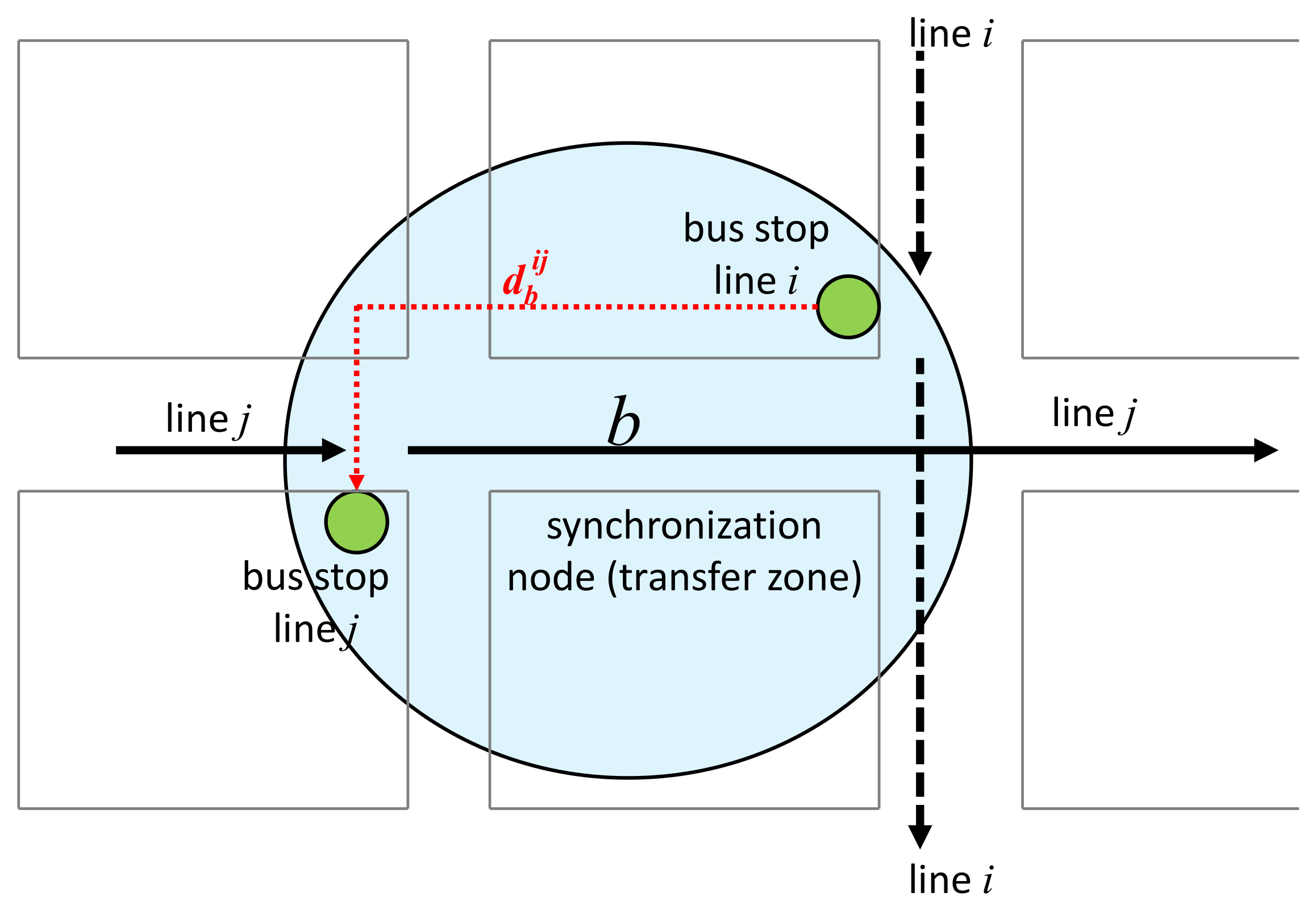
In the considered problem model, the bus network is represented by a set of bus lines and a set of relevant locations (the synchronization nodes or transfer zones), where passengers can transfer from one line to another. Unlike previous formulations of the problem [9,10], in the proposed model, nodes are not just bus stops but wider transfer zones, formed by separated bus stops for lines i and j. This way, the model can include several bus stops for several lines (see a graphical description for two generic lines i and j in Figure 1). The proposed model explicitly includes the distance between the bus stops for lines i and j, $d_b^{i,j}$, drawn in red in Figure 1. For the instances solved in this article, it is assumed that the walking speed of pedestrians is constant $ws=6$ km/h, and the walking time for a distance d between any pair of bus stops is given by $wt=\raisebox{1ex}{$d$}\!\left/ \!\raisebox{-1ex}{$ws$}\right.$.

The proposed problem model is useful for capturing the reality of contemporary intelligent transportation systems, which do not impose a limitation on the number of transfers for passengers and in which transfers are not limited to specific locations. Instead, transfers can be performed at every pair of bus stops, providing flexibility to passengers when planning a trip. This is the case of the intelligent transportation system in Montevideo, Uruguay, which is the case study in this article [7]. In this scenario, the corresponding synchronization problem is more complex, as many realistic transfers options are available to passengers, which in turn may require them to walk between bus stops.

Unlike traditional formulations, the proposed problem model is not focused on maximizing the number of passengers headed from origin to destination, mainly because the main focus is on the user experience when performing transfers, by considering the maximum time passengers are willing to wait for a transfer. This way, the objective function of the optimization model considers the demand of transfers in each transfer zone (pair of bus stops) for all synchronized trips of two bus lines. Previous articles addressing different variants of the timetable synchronization problem have worked under stronger assumptions, i.e., only considering trips for lines to synchronize.

Two cases are distinguished in the proposed model. The case with uniform departing times and the case with non-uniform departing times. These two cases are described next.

In the case with uniform departing times, there are no differences between departing times in the planning period; thus, r and s (trips of line i and line j, respectively) are not relevant for defining the time between consecutive departures (which in fact is constant, i.e., $F_i^1$). This is a realistic assumption when planning for short and medium periods (e.g., in the morning, in the afternoon, in rush hours, etc.). For example, in the case study solved in this article, i.e., the bus network of Montevideo, Uruguay, this assumption holds: in the time period 12:00–14:00 on working days, the time between consecutive buses is almost constant for all lines (the standard deviation of their values is between 0.80% and 1.37%). However, trips of line i and line j are relevant for defining the number of synchronizations and the number of synchronized passengers on each trip.

In the case with non-uniform departing times, the trip number r is relevant to determine synchronizations. The time between consecutive buses is given by $X_r^i-X_{r-1}^i$ for trip r of line i, and the problem formulation must be solved considering the number of trips that are synchronized. When computing the objective function in this model, the demand is split uniformly among the $f_j$ trips of line j. This assumption is also realistic when passengers’ demand has slight variations between consecutive trips. For modeling purposes, we are simply assuming that the planning period is determined because of its regularity. Whenever buses’ interarrival times are uniformly distributed along a planning period, a fairly precise reference weight (i.e., average number of passengers) for each transfer zone is the ratio of the demand of transfers for the considered lines i and j over the number of trips of line i in the planning period T. However, due to the fact that the passengers transferring onto a bus previously alighted from another, they arrive in bursts. There are more accurate formulations for weights in transfer zones [13]. Defining and studying an accurate model to handle variable demands are proposed as future work.

3. Related Work

Timetable synchronization was stated as an important problem for public transportation systems in pioneering research articles by Ceder [3]. Daduna and Voß [14] presented one of the first proposals for synchronizing schedules on public transportation. The authors studied several objective functions, including weighted sum approaches with transfers and maximum waiting time, and proposed metaheuristics for simple problem versions with uniform frequencies. The approach was evaluated over a case study on Berlin and several cities in Germany. In the experiments, tabu search outperformed simulated annealing in randomized instances, and the authors highlighted the trade-off between operation costs and efficiency.

The transit network timetabling problem was studied by Ceder et al. [15] to optimize synchronization events at stops shared by several bus lines, by maximizing the number of simultaneous arrivals. A greedy approach was introduced to define custom timetables, properly selecting nodes from the bus network. The article focused on maximizing simultaneous bus arrivals over small problem instances involving few nodes and lines. A subjective metric was proposed by Fleurent et al. [16] to evaluate synchronizations, including expert knowledge. The proposed synchronization metric was applied to design a heuristic to minimize vehicle operation costs in a case study consisting of small problem instances from Montréal, Canada. Different timetables were found by weighting the components of the cost function.

Shafahi and Khani [17] presented a mixed integer programming model for optimizing transfers in a public transportation network with fixed transfer stations. The problem considered the offset optimization, i.e., setting the departure times of buses, which was solved by an exact method using CPLEX. A second problem variant was formulated, accounting for the extra stopping time of buses at transfer stations. A genetic algorithm was proposed to solve this problem variant over small problem instances involving 14 lines and just three transfer stations. A real case study was presented: the public transportation network in the city of Mashhad, Iran. The proposed methods were able to improve up to 14.5% with a business-as-usual (i.e., no explicit optimization) strategy.

A variant of the the synchronization problem including time-windows between travel times was addressed by Ibarra and Ríos [10]. A multi-start iterated local search (MILS) was applied to solve eight scenarios from the public transportation of Monterrey, Mexico, considering from 4 to 40 nodes. In less than 60 seconds, MILS computed accurate timetables for medium-size instances, regarding both upper bounds and an exact Branch & Bound algorithm. MILS was also applied by Ibarra et al. [11] to solve the multiperiod BSP, to optimize multiple trips of a given set of lines. MILS was able to compute results similar to a variable neighborhood search and a simple population-based algorithm on synthetic instances with few transfer zones. Results for a sample case study using data for a single line of Monterrey demonstrated that maximizing synchronizations for a specific node usually reduces the number of synchronizations for other nodes.

A recent article by Abdolmaleki et al. [18] proposed a model for timetable synchronization assuming a fixed headway for each line. The authors identified specific cases of the problem that are solvable in polynomial time. An approximation algorithm was proposed, based on the maximum directed cut problem. The proposed method was evaluated in a simple network and a large case study in Mashhad, Iran. In turn, a recursive algorithm that executes in quasi-linear time was proposed to minimize the total transfer waiting time in a problem variant that relaxes the fixed headway assumption.

An EA was proposed in a previous article [19] for a specific variant of the BSP, which outperformed real timetables and heuristics. This article extends our previous approach, solving a different BSP variant to determine optimal values for offset and headways, maintaining the number of trips of the real timetable, thus not impacting the provided quality of service.

Regarding the related literature, the approach proposed in this article contributes by considering the extended transfer zones model accounting for transfers between different (geographically separated) bus stops of different lines; by considering the explicit demand of transfer trips for each pair of bus stops that defines a transfer zone to better focus on the quality of service offered to passengers; and by simultaneously adjusting offsets and headways for each line.

4. The Proposed Problem Formulations

This section describes the proposed problem formulations for the considered problem variants.

4.1. Problem Data

The formulation of the studied problem considers:

• The planning period $[0,T]$, expressed in minutes.
• A set of bus lines $I=\{i_1,i_2,\dots ,i_n\}$, whose routes are fixed and known beforehand.
• The total trips needed to perform in order to fulfill the demand for each line i within the planning period $[0,T]$ is $f_i$. The demand considers both direct trips and transfers.
• A set of synchronization nodes, or transfer zones, $B=\{b_1,b_2,\dots ,b_m\}$. Each transfer zone $b\in B$ has three elements <$i,j,d_b^{ij}$>: i and j are the lines that may synchronize, and $d_b^{ij}$ is the distance that separates the bus stops for lines i and j in b. Each b considers two bus stops with transfer demand between lines i and j, as described in Figure 1. The distance $d_b^{ij}$ defines the time that a passenger must walk to transfer from the bus stop of line i to the bus stop of line j in the considered transfer zone.
• A traveling time function $TT:I\times B\to \mathit{Z}$. $T{T}_b^i=TT(i,b)$ defining the time that buses in line i need to travel to reach the transfer zone b. The time is measured from the departure of the line. The traveling time depends of the studied scenario and is affected by several factors such as the maximum allowed speed, the traffic in the city, the travel demands, etc.
• A demand function $P:I\times I\times B\to \mathit{Z}$. $P_b^{ij}=P(i,j,b)$ defines how many passengers perform a transfer from line i to line j in transfer zone b in $[0,T]$. As described in the previous subsection, a hypothesis of uniform demand is assumed. Thus, an effective number transfers from a trip of line i to a trip of line j is properly defined, taking into account the time between two consecutive trips of buses in line i. The uniform demand hypothesis is realistic for short periods, such as in the problem instances defined and solved for the addressed case study.
• The maximum time $W_b^{ij}$ that passengers are willing to wait for line j, after alighting from line i and walking to the corresponding stop of line j in a transfer zone b. Two trips of line i and j are synchronized for transfers if and only if the waiting time of passengers that transfer from line i to line j is lower than or equal to $W_b^{ij}$.
• A set of departing times of each trip r of line i, $X_r^i$, which define the headways of the line as the time between two consecutive trips $F_r^i=(X_r^i-X_{r-1}^i)$. Headway values must be within a range of minimum ($h_i$) and maximum ($H_i$) headways for that line. Both extreme values are defined by the city administration or the bus system operator. The offset of each line is the departing time of the first trip of the line ($X_1^i$). Without losing generality, the model assumes $X_0^i=0$. All trips of each line must start within the planning period $[0,T]$ (i.e., $X_{f_i}^i\le T$).

Considering the previously defined elements, two variants of the BSP are formulated, accounting for the optimization of just offsets and both offsets and headways for each line, respectively. The next subsections describe these two problem variants.

4.2. Problem Variant #1: Offset Optimization

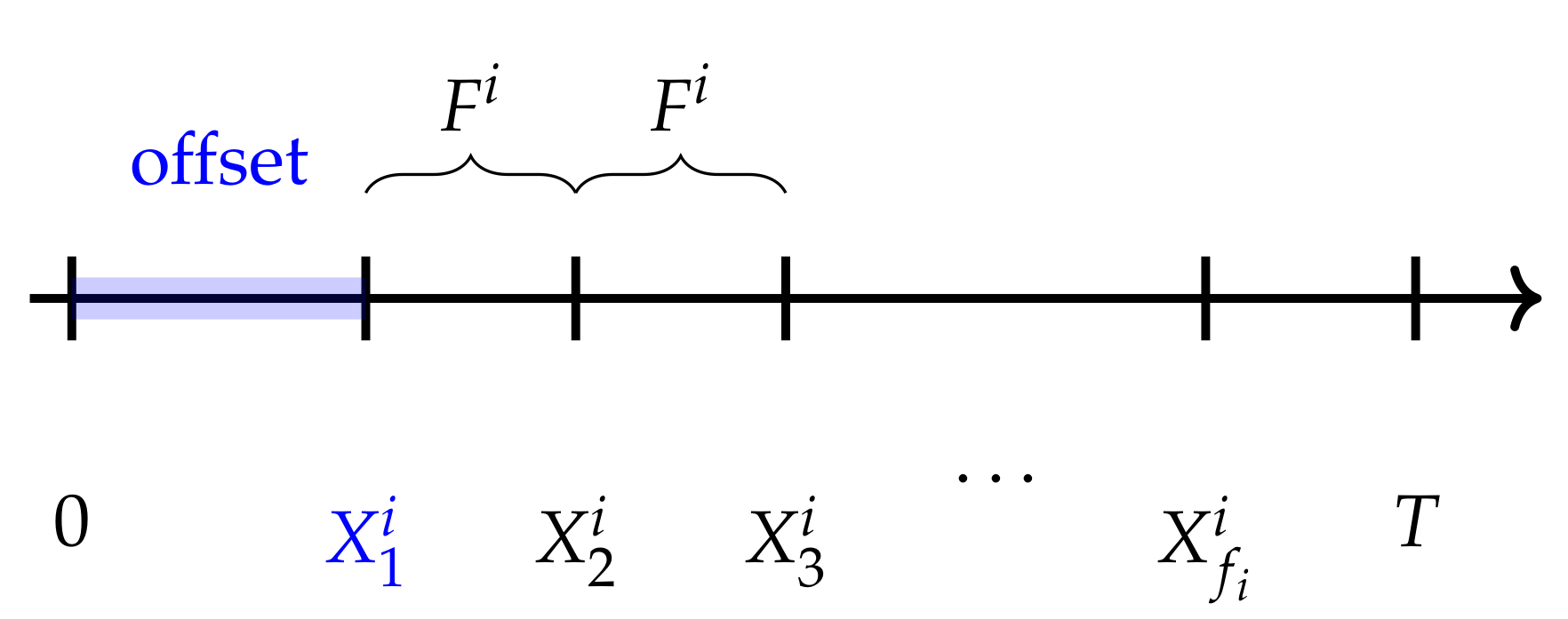
The first problem variant focuses on optimizing the offsets (i.e., the departing time of the first trip of each line). Subsequent departing times are fixed by the reference value defined by the city administration ($F^i$). Thus, the control variables of the problem are the offset of each line ($X_1^i$), which defines the whole set of departing times for all trips of each line. Auxiliary variables are needed to capture the synchronization events in each transfer zone. Binary variables $Z_{rsb}^{ij}$ take a value 1 when trip r of line i and trip s of line j are synchronized in node b (i.e., trip r of line i arrives before trip s of line j and allows passengers to complete the transfer, i.e., walk between the corresponding bus stops and wait less than the waiting threshold for that transfer, $W_b^{ij}$). To guarantee that all lines perform the required number of trips in the planning period, possible values for the offset are limited to the interval $[0,T(\mathrm{mod}{F}^i)]$ (see a graphical description in Figure 2).

The mathematical model of BSP variant #1 as a mixed integer programming (MIP) problem is formulated in Equations (1)–(5).

$$\begin{array}{cc}\hfill \mathrm{maximize}& {\displaystyle \sum _{b\in B}(\sum _{r=1}^{f_i}\sum _{s=1}^{f_j}{Z}_{rsb}^{ij})·\frac{P_b^{ij}\times F^i}{T}}\hfill \end{array}$$

(1)

$$\begin{array}{ccc}\hfill \mathrm{subject} \mathrm{to}& Z_{rsb}^{ij}\le 1+\frac{(A_{rb}^i+d_b^{ij}+W_b^{ij})-A_{sb}^j}{M},\hfill & \hfill \begin{array}{c}\forall b=<i,j,d_b^{ij}>\in B,\hfill \\ 1\le r\le f_i,1\le s\le f_j,\hfill \end{array}\end{array}$$

(2)

$$\begin{array}{ccc}& Z_{rsb}^{ij}\le 1+\frac{A_{sb}^j-(A_{rb}^i+d_b^{ij})}{M},\hfill & \hfill \begin{array}{c}\forall b=<i,j,d_b^{ij}>\in B,\hfill \\ 1\le r\le f_i,1\le s\le f_j,\hfill \end{array}\\ & \mathrm{with}{A}_{rb}^i=X_1^i+(r-1)F^i+T{T}_b^i\mathrm{and}\hfill & \hfill A_{sb}^j=X_1^j+(s-1)F^j+T{T}_b^j\end{array}$$

(3)

$$\begin{array}{ccc}& 0\le X_1^i\le min(H_i,T(\mathrm{mod}{F}^i)),\hfill & \hfill \forall i\in I\end{array}$$

(4)

$$\begin{array}{cc}& Z_{rsb}^{ij}\in \{0,1\},\forall i\in I\hfill \end{array}$$

(5)

The optimization problem formulates the maximization of the number of successful transfers completed in the planning period in every transfer zone (the objective function in Equation (1)). The expression ${\sum }_{r=1}^{f_i}{\sum }_{s=1}^{f_j}{Z}_{rsb}^{ij}$ is the total number of successful connections between trips of each pair of lines i and j in each transfer zone b. Assuming a uniform demand hypothesis, the number of transfers from a trip of line i to a trip of line j in the planning period is $P_b^{ij}\times F^i/T$. Equations (2)–(5) define the problem constraints.

Equation (1) states that the optimization will seek to activate synchronization variables $Z_{rsb}^{ij}$—as many as possible. Constraints determine that variables $Z_{rsb}^{ij}$ only take the value 1 if the corresponding transfer is synchronized. In Equations (2) and (3), the arrival time of trip r of line i to transfer zone b is $A_{rb}^i$, and the arrival time of trip s of line j to transfer zone b is $A_{sb}^j$. For an interpretation of constraint (2), consider that the limit time $A_r^i+d_b^{ij}+W_b^{ij}$ defines the maximum time passengers are willing to wait for a transfer between trip r of line i and trip s of line j at transfer zone b. Whenever the arrival time of trip s of line j does not surpass that limit, the right-hand side of Equation (2) is greater (or equal) to 1, so this is the only case when $Z_{rsb}^{ij}$ (the synchronization variable) is allowed to take the value 1. Furthermore, it is also necessary for passengers alighting from trip r of line i to walk to the transfer point (arriving at time $A_{rb}^i+d_b^{ij}$) before trip s of line j arrives (at time $A_{sb}^j$). Otherwise, passengers will not complete the transfer on time. This second condition, when met, also allows $Z_{rsb}^{ij}$ to be set to 1, as the right term of constraints in Equation (3) is positive. To date, there is a potential issue when non-synchronized trips lead to negative values on the right term of Equation (3), which produces unfeasible constraints. The formulation only needs one value, $(A_{rb}^i+d_b^{ij}+W_b^{ij})-A_{sb}^j$ or $A_{sb}^j-(A_{rb}^i+d_b^{ij})$, to be lower than zero, so the synchronization variable $Z_{rsb}^{ij}$ is deactivated. Thus, it is enough to introduce a constant value M, large enough to guarantee that both Equations (2) and (3) are always feasible. In a real solver implementation, considering large values of M might cause numerical stability problems. Thus, appropriate and relatively low values for M are computed as the maximum value within the union of sets $\{(H_i(j)+(f_i(j)-1)\times \Delta X^j+T{T}_b^j)-(T{T}_b^i+d_b^{ij}+W_b^{ij})\}$ and $\{(H_i(i)+(f_i(i)-1)\times \Delta X^i+T{T}_b^i+d_b^{ij})-T{T}_b^j\}$ for all transfer zones $binB$. These values of M can be easily calculated during the process of crafting the MIP formulation before using any solver implementation, since finding M is a polynomial complexity problem. Equation (4) indicates that the maximum value for the offset of each line is the minimum between $T(\mathrm{mod}{F}^i)$ and the maximum headway $H_i$. No constraints are defined over headways, since a fixed frequency $F^i$, which satisfies the bounds for headways, is assumed for all subsequent trips. Finally, Equation (5) defines that decision variables $Z_{rsb}^{ij}$ are within the domain of binary variables.

Without losing generality, the proposed problem formulation assumes that $F^j>W_b^{ij}$, $\forall j\in I$, i.e., headways of bus lines are larger than the waiting time thresholds for users. The case where $F^j\le W_b^{ij}$ corresponds to a scenario in which the headway of line j is lower than the time users are willing to wait; thus, all transfers with line j would be synchronized, and they would not be part of the problem to solve (i.e., those lines can be removed for the specific problem instance to solve).

4.3. Problem Variant #2: Headways Optimization

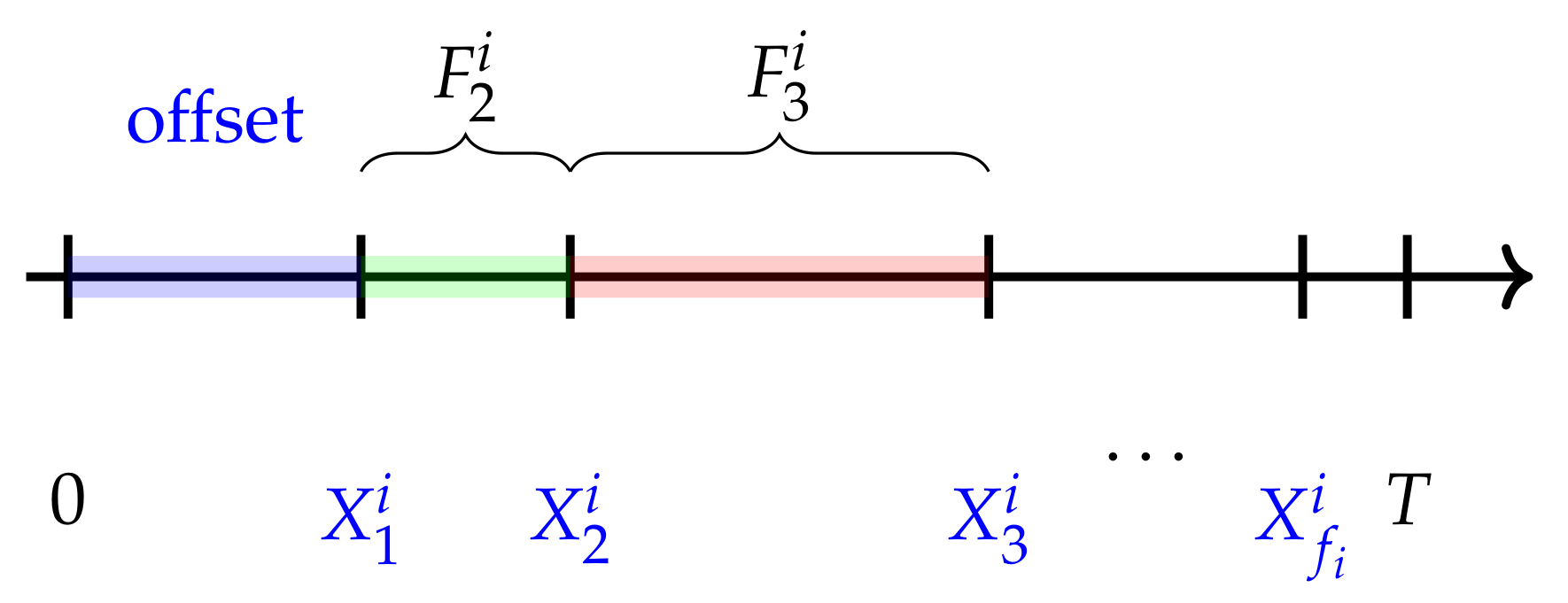
The second problem variant proposes optimizing not only the offsets of each line but also the headways of each line. Headways are allowed to vary within a fixed range of the reference value $F^i$. The interval for variation is defined by $F^i(1-\alpha )\le X_r^i-X_{r-1}^i\le F^i(1+\alpha ),\forall r\in 1,2,\dots ,f_i$. To work under the assumption of maintaining an appropriate quality of service for the transportation system, which is assumed to be fairly provided by the current situation (i.e., using the reference values for the time difference between consecutive trips of each line), small values of $\alpha$ are considered (see a graphical description in Figure 3).

The mathematical model of BSP variant #2 as an MIP problem is formulated in Equations (6)–(13).

$$\begin{array}{cc}\hfill \mathrm{maximize}& {\displaystyle \sum _{b\in B}(\sum _{r=1}^{f_i}\sum _{s=1}^{f_j}{Z}_{rsb}^{ij})·\frac{P_b^{ij}\times (X_r^i-X_{r-1}^i)}{T}}\hfill \end{array}$$

(6)

$$\begin{array}{ccc}\hfill \mathrm{subject} \mathrm{to}& Z_{rsb}^{ij}\le 1+\frac{(A_{rb}^i+d_b^{ij}+W_b^{ij})-A_{sb}^j}{M},\hfill & \hfill \begin{array}{c}\forall b=<i,j,d_b^{ij}>\in B,\hfill \\ 1\le r\le f_i,1\le s\le f_j,\hfill \end{array}\end{array}$$

(7)

$$\begin{array}{ccc}& Z_{rsb}^{ij}\le 1+\frac{A_{sb}^j-(A_{rb}^i+d_b^{ij})}{M},\hfill & \hfill \begin{array}{c}\forall b=<i,j,d_b^{ij}>\in B,\hfill \\ 1\le r\le f_i,1\le s\le f_j,\hfill \end{array}\\ & \mathrm{with}{A}_{rb}^i=X_r^i+T{T}_b^i,A_{sb}^j=X_s^j+T{T}_b^j\hfill \end{array}$$

(8)

$$\begin{array}{cc}& \sum _{s=1}^{f_j}{Z}_{rsb}^{ij}\le 1,\forall i,j\in I,1\le r\le f_i\hfill \end{array}$$

(9)

$$\begin{array}{ccc}& max(F^i(1-\alpha ),h_i)\le X_r^i-X_{r-1}^i,\hfill & \hfill \forall r\in 2,..,f_i\end{array}$$

(10)

$$\begin{array}{ccc}& X_r^i-X_{r-1}^i\le min(F^i(1+\alpha ),H_i),\hfill & \hfill \forall r\in 2,..,f_i\end{array}$$

(11)

$$\begin{array}{cc}& T-H_i\le X_{f_i}^i\le T,\forall i\in I\hfill \end{array}$$

(12)

$$\begin{array}{cc}& Z_{rsb}^{ij}\in \{0,1\},0\le X_1^i\le min(H_i,mod(T,F^i))\hfill \end{array}$$

(13)

In Equations (6)–(13), $X_r^i$ is the time of departure of trip r of line i, and $F^i$ is the reference value for the time difference between consecutive trips of line i, as defined in problem variant #1. In turn, $\alpha \in [0,1]$ is the coefficient used for defining the allowed deviation of times between buses from the reference value $F^i$. Finally, $X_{f_i}^i$ is the departing time of the last trips of the line i.

The objective function is Equation (6), i.e., maximizing the number of successful transfers completed in every transfer zone in the planning period. In this case, the demand is split considering the (flexible) time between consecutive buses of line i (i.e., $X_r^i-X_{r-1}^i$). Equations (7)–(13) formulate the problem constraints. Equations (7) and (8) define a synchronization, as in the previous problem formulation.

Equation (9) guarantees that every trip r of line i synchronizes with, at most, one trip s of line j. The last point is necessary because headways are part of the control variables in this case. In the previous model, headways were known in advance, so they could be pre-filtered in the case where a headway was lower than the maximum time passengers are willing to wait at some stop. Conversely, in this model, Equation (9) prevents us from counting such synchronizations more than once. Constraints in Equations (10) and (11) impose the limits for headways, according to the allowed variation $\alpha$. Constraints in Equation (12) guarantee that the last trip is within the specified maximum range. Finally, Equation (13) defines the domain for decision variables $Z_{rsb}^{ij}$.

The formulation in Equations (6)–(13) intuitively extends the previous to incorporate headways as control variables, but it has the drawback of being quadratic in its objective function due to the product of $Z_{rsb}^{ij}(X_r^i-X_{r-1}^i)$. However, it is linearized by a change of variables and additional constraints. Let $y_{rsb}^{ij}$ be as $Z_{rsb}^{ij}(X_r^i-X_{r-1}^i)$ in (6), so the objective turns out to be ${\displaystyle \frac{1}{T}\sum _{b\in B}\sum _{r=1}^{f_i}\sum _{s=1}^{f_j}{y}_{rsb}^{ij}·P_b^{ij}}$, which is linear. Moreover, two equations per each $y_{rsb}^{ij}$ variable must be included: $y_{rsb}^{ij}\le (X_r^i-X_{r-1}^i)$ and $y_{rsb}^{ij}\le H_i·Z_{rsb}^{ij}$. Within a maximization problem, variables $y_{rsb}^{ij}$ will take a value as high as possible. $H_i$ is an upper bound for $(X_r^i-X_{r-1}^i)$ because of Equation (11), so whenever $Z_{rsb}^{ij}=1$, the second equation results, $y_{rsb}^{ij}\le H_i$, and it is the first equation that guarantees y’s value to be $(X_r^i-X_{r-1}^i)$ at most, which is then exactly the value that the variable $y_{rsb}^{ij}$ will take. Conversely, when $Z_{rsb}^{ij}=0$, the second equation forces $y_{rsb}^{ij}$ to be 0. This behavior replicates that of $Z_{rsb}^{ij}(X_r^i-X_{r-1}^i)$’s product, so the change of variables is equivalent and linear.

Table 1. Summary of the proposed BSP variants.

Problem	Decision Variables	Model (Objective, Constraints)
variant #1	$X_1^i$ (offset)	Equations (1)–(5)
variant #2	$X_1^i$ (offset), $X_s^i$ (headways, within range)	Equations (6)–(13)

summarizes both problem variants. Variables $X_1^i$ (i.e., offsets) are the control variables in both proposed problem variants, while the latter adds new control variables $X_r^i$ with $r>1$. The difference is semantic rather than substantive, and we refer to them as $X_r^i$ in general. The group of variables $Z_{rsb}^{ij}$ are auxiliary in both proposed problem variants. They are used to identify synchronizations as an outcome of control variable $X_r^i$ values. These variables are only meaningful when stated as Boolean variables, a condition that must be explicitly set in the formulation since it is not achieved otherwise. Finally, problem variant #2 introduces $y_{rsb}^{ij}$ variables, which are also auxiliary and number as many as those of $Z_{rsb}^{ij}$. They are used to obtain to a purely linear alternative formulation for the second problem variant.

Unlike $Z_{rsb}^{ij}$ variables, the domain of $X_r^i$ and $y_{rsb}^{ij}$ is that of the real numbers, since their values are a consequence of active constraints in an optimization process. However, whenever parameters that define an instance are integers, optimal $X_1^i$ values Equations (1)–(5) are to be integers as well, as they are the result of pushing the objective function variables against integer constraints. The situation is not so for Equations (6)–(13), because $\alpha$ values greater than 0 generally lead to non-integer bounds in both proposed problem variants.

5. Exact and Evolutionary Computation Methods for the BSP

This section presents the exact and evolutionary computation approaches developed to address the BSP, considering extended transfer zones.

5.1. Mathematical Programming

The exact method for solving the formulated model was developed by combining several tools. Each instance in the input dataset was imported into MATLAB matrices, just as it was for each solution (externally found). In this way, results could be easily analyzed, debugged, and post-processed. The software version of MATLAB is R2015a-8.5.0.

Some parameters of the models formulated in both proposed problem variants are to be computed during the MIP construction itself. The most notorious is the value of the parameter M, which has to be large enough to prevent (2), (3) or (7), (8) from being unfeasible but not so large to lead to numerical issues. Because of this, we decided not to use AMPL or other algebraic modeling language to feed the solver. Instead, we developed a C++ program to read instances in the input dataset and convert them to CPLEX LP-format.

IBM(R) ILOG(R) CPLEX(R) Interactive Optimizer 12.6.3.0 was used as the optimization tool. The default GAP tolerance for the MIP solver is 0.01%. This corresponds to the relative distance between the best integer solution found and the best upper bound estimated up to that moment: $(f(x)-bestBound)/f(x)$, where x is a solution, $f(x)$ is its objective function value, and $bestBound$ is the lowest upper bound found for the optimum value.

5.2. Evolutionary Algorithm

The EA was developed using the Malva library (github.com/themalvaproject, accessed on 15 June 2021) in the C++ programming language. The main implementation details are described in the next subsections.

Solution Encoding

For both problem variants, candidate solutions are represented using integer vectors. Next, both representations are explained.

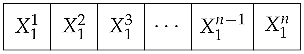
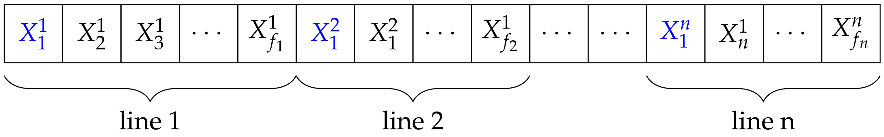
Problem variant #1: offset optimization. For problem variant #1, each integer value in the solution representation indicates the offset for each bus line, i.e., the time elapsed between time zero (start of the planning period) and the time when the first trip of the line departs. A candidate solution of the BSP is represented by a vector $X=\{X_1^1,X_1^2,\dots X_1^n\}$ (n is the number of lines in the instance), $X_0^i\in {\mathit{Z}}^{+}$, and $0\le X_0^i\le Tmod{H}^i$. Figure 4 describes the solution representation for a problem instance with n bus lines.

Problem variant 2: headways optimization. For problem variant #2, integer values in the solution representation represent, for each bus line, the offset (in minutes) and the subsequent headway values (also in minutes). A candidate solution of the BSP is represented by a vector $X=\{X_1^1,X_2^1,\cdots ,X_{f_1}^1,X_1^2,X_2^2\cdots ,X_{f_2}^2,\cdots ,X_1^n,\cdots ,X_1^n,\cdots ,X_{f_n}^n$}, where $X_0^i\in {\mathit{Z}}^{+}\cup 0$, and $X_{k_i}^i\in {\mathit{Z}}^{+}$, with $k_i\in \{1,\cdots ,f_i\}$. Figure 5 describes the solution representation for a problem instance with n bus lines (offset values for each line are marked in blue font).

Evolution model. The EA follows the ($\mu +\lambda$) evolution model [20]. $\lambda$ offsprings are generated from $\mu$ parents, and all compete among themselves to select the solutions to include in the population in a new generation. The ($\mu +\lambda$) evolution model computed better and more diverse solutions than a standard generational model in configuration experiments.

Initialization operator. The initialization generates random solutions, selecting integer values within the corresponding ranges and taking into account the problem constraints. The random initialization operator is conceived to generate an appropriate diversity for the evolutionary process.

Selection operator. A tournament method is used for selecting individuals during the evolutionary search. A tournament size of three individuals was used (just one individual survives). The tournament operator outperformed the standard proportional selection in configuration experiments, providing a proper selection pressure for candidate solutions during the evolutionary process.

Recombination operator. An ad hoc variant of the well-known two-point crossover operator was designed. Crossover points are randomly selected in $[1,n$−$1]$, and information from both parents is exchanged between the crossover points. The main idea is to maintain those features of bus lines synchronized in the parent to be used as relevant information for offspring generation. The recombination probability is $p_R$. A correction procedure is applied to guarantee the feasibility of the generated solutions by properly shifting conflicting offset and/or headway values.

Mutation operator. An ad hoc variant of Gaussian mutation is applied. Selected position(s) in an individual are changed according to a Gaussian distribution and considering the limits (minimum and maximum) defined for both offsets and headways of each line. The mutation probability is $p_M$.

6. Experimental Evaluation

The experimental analysis of the exact and evolutionary methods for the BSP is reported in this section.

6.1. Methodology

This subsection describes the methodology applied for the experimental evaluation of the proposed methods to solve the BSP.

6.1.1. Problem Instances

The experimental evaluation considered realistic problem instances, generated using real information from the case study, i.e., the STM in Montevideo, Uruguay.

Several data sources were considered to gather information to build the BSP instances. All the information about the bus network (lines, routes, real timetables, bus stops locations, etc.) was retrieved from the National Open Data Catalog (catalogodatos.gub.uy, accessed on 15 June 2021). The real information about transfer demands was provided by the city administration. All the gathered data were analyzed applying urban data analysis [7]. Several elements define the scenario and the problem instances built:

• The starting time was set to 12:00 p.m., and the final time was set to 2:00 p.m., including one of the two peak hours occurring in a working day for the public transportation system in Montevideo [21].
• The transfer demand function (P) is generated from real information registered by the smart cards of the STM.
• The transfer zones are selected from the pairs of bus stops with the largest demand of registered transfers for the period; all pairs are candidates to be selected in the created BSP instances; the number of considered transfer zones is 170.
• The bus lines are those connecting the considered transfer zones; a total number of 250 lines are considered.
• The time traveling function ($TT$) is computed by processing the real GPS data from the operating vehicles for each line;
• The walking time function is defined by the product of the estimated pedestrian speed (6 km/h) and the distance between bus stops in each transfer zone; the distance is computed using geospatial analysis.
• The maximum waiting time (W) is $\lambda H$; five values of $\lambda$ are considered ($\lambda \in$ [0.3, 0.5, 0.7, 0.9] to define BSP instances with different tolerance levels.

A total number of 75 BSP instances are defined, of three different dimensions (30, 70, and 110 transfer zones), using the real information of buses operating in the STM of Montevideo, Uruguay. Problem instances are named as [NP].[NL].[$\lambda$].[id]: NP = n the number of transfer zones, NL = m the number of bus lines, $\lambda$ the tolerance to define the maximum waiting time (percentage), and id is a number to differentiate instances with the same values of the other parameters. Problem instances are publicly available at www.fing.edu.uy/inco/grupos/cecal/hpc/bus-sync/, accessed on 15 June 2021.

6.1.2. Execution Platform

Experiments were carried out on a Quad-core Xeon E5430 at 2.66GHz, 8 GB RAM, from the high-performance computing infrastructure of the National Supercomputing Center (Cluster-UY), Uruguay [22].

6.1.3. Baseline Solution for the Comparison

A significant solution to be used as baseline for the comparison is the real timetable used in the transportation system of Montevideo. This solution determines the current level of service regarding both direct trips and transfers. The real timetable does not apply an explicit synchronization approach for transfers. The first trip of each line departs when the planning period starts, and subsequent trips depart according to the real predefined headways for each line. The comparison with the real timetable allows determining the advantages of the explicit optimization approaches proposed for the studied BSP variants.

6.1.4. Statistical Analysis and Metrics

The effectiveness of the proposed EA is assessed via proper statistical analysis. For every problem instance and experiment, 30 independent executions (i.e., using a different seed for the random numbers generator) were performed. Then, a three-step analysis is applied to study the fitness results distributions:

• Normality check. The Shapiro–Wilk statistical test is applied to determine if the results distribution is modeled by a normal distribution, i.e., computing the likeliness of the underlying randomness to be normally distributed.
• Mean rank comparison (for parametric configuration analysis). The Friedman rank statistical test is applied to detect/analyze the differences in the distributions of fitness values across multiple executions.
• Pairwise comparison of distributions. The Kruskal–Wallis non-parametric test is applied to determine if the differences between two parameter configurations have statistic significance.
• Boxplots are used for results visualization and graphical comparison. Relevant order statistics are computed and reported: first quartile (Q1), third quartile (Q3), median, minimum, and maximum values, since the Shapiro–Wilk test confirmed that the results do not follow a normal distribution. The interquartile range (IQR) is used as a measure of statistical dispersion, as usual for non-normal distributions.

Several metrics are used for evaluating the exact and the evolutionary approach: (i) the number of successfully synchronized trips for passengers (i.e., the objective function defined in Equations (1) and (6)), (ii) the improvements over the real solution, and (iii) the average waiting for transfers in a transfer zone.

6.1.5. Parameter Setting

Exact Mathematical Programming. The default set of parameters of CPLEX was used to find exact solutions, except for the timeout parameter, which was set to 7200 seconds. Variant #2 with $\alpha =0$ is equivalent to variant #1, where headways are fixed and equal to $F^i$. However, problem formulations are not equal nor are the proposed methods to solve them. Variant #2 implies significantly more variables than variant #1, so it is worth checking that algorithms are also able to rapidly find solutions when $\alpha =0$. Such instances were solved within a few seconds, so the timeout limit only applies for $\alpha =0.3$. It was verified, though, that the performance of the more general variant #2 is quite good for very low values of $\alpha$, comparable to the performance of the much simpler version #1. Runtimes degrade for higher values of $\alpha$, and in fact, the best solutions found for $\alpha =0.3$ were not proven to be optimal according to the defined tolerance for the MIP solver (0.01%). There is room to explore changes in parameters in order to improve performance, which is appointed as a future line of work.

Evolutionary algorithm. Since EAs are non-deterministic, parameter configuration analysis is mandatory to find the proper combination of parameter values to compute the best results. Studied parameters included population size (ps), recombination probability ($p_R$), and mutation probability ($p_M$). Experiments were performed on five small problem instances with different features to avoid bias. Candidate values considered for each parameter were $ps\in \{15,25,50\}$, $p_R\in \{0.5,0.75,0.9\}$, and $p_M\in \{0.001,0.01,0.1\}$.

A summary of the results obtained in the analysis of the population size is presented in

Table 2. Analysis of the population size.

	Average Fitness
ps	30.37.30.1	30.37.50.1	30.37.70.1	30.37.90.1	30.37.100.1
15	251.96	267.15	286.97	295.06	296.51
25	253.78	266.50	288.01	295.45	297.48
50	253.70	271.89	287.39	295.37	297.19
	Friedman Rank ($\mathit{p}$-Value < ${\mathbf{10}}^{-\mathbf{3}}$)
ps	30.37.30.1	30.37.50.1	30.37.70.1	30.37.90.1	30.37.100.1
15	3	2	3	3	3
25	1	3	1	1	1
50	2	1	2	2	2
	Best Fitness
ps	30.37.30.1	30.37.50.1	30.37.70.1	30.37.90.1	30.37.100.1
15	260.71	276.41	291.07	296.69	298.31
25	260.94	275.33	291.72	297.95	298.46
50	262.18	273.62	290.06	296.09	298.22
	Friedman Rank ($\mathit{p}$-Value < ${\mathbf{10}}^{-\mathbf{3}}$)
ps	30.37.30.1	30.37.50.1	30.37.70.1	30.37.90.1	30.37.100.1
15	3	1	2	2	2
25	2	2	1	1	1
50	1	3	3	3	3

. Results of median and best fitness values are reported for each population size. The Friedman rank test is applied to analyze the results distribution.

Results in Table 2 demonstrate that the best results were computed using a population size of 25 individuals. Using a larger population size turned to be counterproductive for the EA, since suboptimal solutions dominate quickly and results do not improve in the long term.

Table 3. Analysis of the recombination and mutation probabilities in the proposed EA.

			Fitness
id	$p_R$	$p_M$	30.37.30.1	30.37.50.1	30.37.70.1	30.37.90.1	30.37.100.1
C1	0.5	0.010	253.18	263.90	285.82	292.03	294.97
C2	0.5	0.005	263.30	274.21	293.15	298.19	298.79
C3	0.5	0.001	253.99	267.70	287.67	295.56	297.06
C4	0.75	0.010	250.67	268.65	286.70	293.12	294.50
C5	0.75	0.005	262.91	276.65	291.69	296.48	298.25
C6	0.75	0.001	250.32	270.05	284.09	292.87	294.89
C7	0.9	0.010	255.12	269.66	289.43	293.91	296.06
C8	0.9	0.005	260.94	275.33	291.72	297.95	298.46
C9	0.9	0.001	256.80	269.87	288.57	296.71	297.45
			Friedman Rank
id	$p_R$	$p_M$	30.37.30.1	30.37.50.1	30.37.70.1	30.37.90.1	30.37.100.1	avg.
C1	0.50	0.01	7	9	8	9	7	8.0
C2	0.50	0.005	1	3	1	1	1	1.4
C3	0.50	0.001	6	8	6	5	5	6.0
C4	0.75	0.01	8	7	7	7	9	7.6
C5	0.75	0.005	2	1	3	4	3	2.6
C6	0.75	0.001	9	4	9	8	8	7.6
C7	0.90	0.01	5	6	4	6	6	5.4
C8	0.90	0.005	3	2	2	2	2	2.2
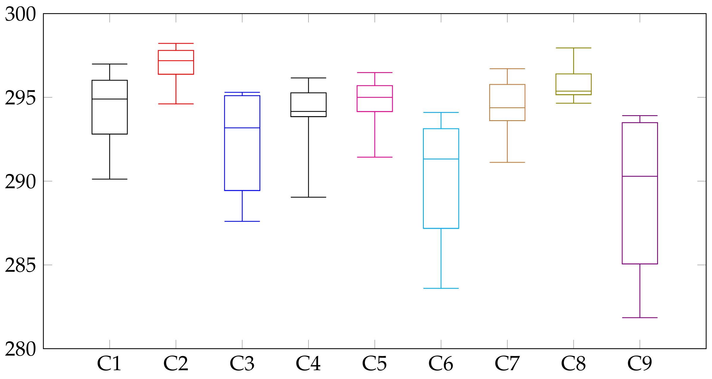
C9	0.90	0.001	4	5	5	3	4	4.2

reports the best fitness values and the Friedman ranks of the nine configurations (C1, …, C9) considered in the analysis of the recombination and mutation probabilities. The p-value of the Friedman rank was below ${10}^{-3}$, thus assuring statistical significance of the results. In turn, the boxplots in Figure 6 graphically compare the median, best, worst, Q1, and Q3 values obtained for each studied configuration in the problem instance, which is representative of the results computed for other instances too. According to the reported metrics, the best results were obtained with configuration C2, i.e., setting PS = 25, $p_R$ = $0.5$, and $p_M$$=$$0.005$. Configuration C2 systematically obtained the best Friedman ranking in all but one of the studied problem instances.

6.2. Numerical Results

This subsection reports the numerical results of the proposed methods for the BSP and the comparison with the baseline real timetable for both studied problem variants.

6.2.1. Problem Variant #1: Offset Optimization

Table 4. Summary of results: exact and EA for BSP variant #1.

Scenario	EA	Exact	Real	EA vs. Exact	EA vs. Real	Exact vs. Real
30.37.100.1	265.76	265.76	245.33	0.00%	8.3%	8.3%
30.37.30.1	171.12	171.12	102.88	0.00%	66.3%	66.3%
30.37.50.1	203.52	203.58	165.28	−0.03%	23.1%	23.2%
30.37.70.1	252.22	252.22	219.60	0.00%	14.9%	14.9%
30.37.90.1	260.68	260.68	245.33	0.00%	6.3%	6.3%
30.40.100.0	205.68	205.68	187.57	0.00%	9.7%	9.7%
30.40.100.4	223.17	223.17	204.49	0.00%	9.1%	9.1%
30.40.30.0	131.76	132.13	82.83	−0.28%	59.1%	59.5%
30.40.30.4	143.98	143.98	98.36	0.00%	46.4%	46.4%
30.40.50.0	162.15	162.17	122.31	−0.01%	32.6%	32.6%
30.40.50.4	169.66	169.66	123.83	0.00%	37.0%	37.0%
30.40.70.0	195.54	195.54	166.10	0.00%	17.7%	17.7%
30.40.70.4	208.99	208.99	179.18	0.00%	16.6%	16.6%
30.40.90.0	205.68	205.68	187.57	0.00%	9.7%	9.7%
30.40.90.4	223.12	223.12	202.69	0.00%	10.1%	10.1%
30.41.100.2	247.59	247.59	224.50	0.00%	10.3%	10.3%
30.41.30.2	154.11	154.20	95.89	−0.06%	60.7%	60.8%
30.41.50.2	186.95	187.35	145.39	−0.21%	28.6%	28.9%
30.41.70.2	236.50	236.50	195.47	0.00%	21.0%	21.0%
30.41.90.2	247.59	247.59	224.05	0.00%	10.5%	10.5%
30.42.100.3	231.13	231.13	211.67	0.00%	9.2%	9.2%
30.42.30.3	138.83	138.83	93.27	0.00%	48.8%	48.8%
30.42.50.3	168.64	168.64	142.38	0.00%	18.4%	18.4%
30.42.70.3	212.78	212.78	187.80	0.00%	13.3%	13.3%
30.42.90.3	230.98	230.98	211.12	0.00%	9.4%	9.4%
70.60.100.1	540.41	540.41	492.20	0.00%	9.8%	9.8%
70.60.30.1	332.11	333.02	211.56	−0.27%	57.0%	57.4%
70.60.50.1	404.30	406.61	310.96	−0.57%	30.0%	30.8%
70.60.70.1	509.60	509.60	435.28	0.00%	17.1%	17.1%
70.60.90.1	539.53	539.53	491.70	0.00%	9.7%	9.7%
70.62.100.3	522.34	522.34	479.58	0.00%	8.9%	8.9%
70.62.30.3	306.14	309.02	207.12	−0.93%	47.8%	49.2%
70.62.50.3	388.99	389.69	321.41	−0.18%	21.0%	21.2%
70.62.70.3	486.82	486.82	417.53	0.00%	16.6%	16.6%
70.62.90.3	521.82	521.82	478.46	0.00%	9.1%	9.1%
70.63.100.2	525.90	525.90	478.87	0.00%	9.8%	9.8%
70.63.30.2	332.06	334.45	200.77	−0.55%	65.7%	66.6%
70.63.50.2	405.90	405.90	316.53	0.00%	28.2%	28.2%
70.63.70.2	497.84	497.84	427.21	0.00%	16.5%	16.5%
70.63.90.2	525.90	525.90	477.09	0.00%	10.2%	10.2%
70.67.100.0	487.42	487.42	440.27	0.00%	10.7%	10.7%
70.67.30.0	304.60	304.85	203.81	−0.08%	49.5%	49.6%
70.67.50.0	374.91	374.98	289.39	−0.02%	29.6%	29.6%
70.67.70.0	459.73	459.93	386.96	−0.04%	18.8%	18.9%
70.67.90.0	487.42	487.42	440.27	0.00%	10.7%	10.7%
70.69.100.4	505.15	505.15	456.10	0.00%	10.8%	10.8%
70.69.30.4	322.57	322.57	209.04	0.00%	54.3%	54.3%
70.69.50.4	385.63	385.63	295.16	0.00%	30.7%	30.7%
70.69.70.4	475.36	475.36	408.63	0.00%	16.3%	16.3%
70.69.90.4	504.20	504.20	454.31	0.00%	11.0%	11.0%
110.76.100.2	777.19	777.19	706.18	0.00%	10.1%	10.1%
110.76.30.2	487.71	489.13	298.20	−0.29%	63.6%	64.0%
110.76.50.2	591.50	591.50	465.58	0.00%	27.0%	27.0%
110.76.70.2	731.20	731.20	631.71	0.00%	15.7%	15.7%
110.76.90.2	777.06	777.06	703.90	0.00%	10.4%	10.4%
110.78.100.0	806.58	806.58	728.94	0.00%	10.7%	10.7%
110.78.100.1	826.45	826.45	752.16	0.00%	9.9%	9.9%
110.78.100.3	803.13	803.13	731.61	0.00%	9.8%	9.8%
110.78.30.0	487.92	490.34	315.02	−0.49%	54.9%	55.7%
110.78.30.1	507.28	511.37	311.43	−0.80%	62.9%	64.2%
110.78.30.3	499.39	499.39	307.45	0.00%	62.4%	62.4%
110.78.50.0	606.89	610.36	461.39	−0.57%	31.5%	32.3%
110.78.50.1	623.89	623.89	467.20	0.00%	33.5%	33.5%
110.78.50.3	605.72	609.60	472.20	−0.64%	28.3%	29.1%
110.78.70.0	753.93	754.26	648.61	−0.04%	16.2%	16.3%
110.78.70.1	775.14	775.14	659.51	0.00%	17.5%	17.5%
110.78.70.3	753.11	753.76	635.61	−0.09%	18.5%	18.6%
110.78.90.0	805.77	805.77	727.38	0.00%	10.8%	10.8%
110.78.90.1	824.47	824.47	751.09	0.00%	9.8%	9.8%
110.78.90.3	802.42	802.42	729.99	0.00%	9.9%	9.9%
110.83.100.4	779.09	779.09	713.79	0.00%	9.1%	9.1%
110.83.30.4	501.43	501.43	305.51	0.00%	64.1%	64.1%
110.83.50.4	593.89	593.89	464.88	0.00%	27.8%	27.8%
110.83.70.4	730.68	730.68	635.29	0.00%	15.0%	15.0%
110.83.90.4	778.09	778.09	711.49	0.00%	9.4%	9.4%

presents the objective function values achieved by the exact and the EA for the studied BSP instances for variant #1 (offset optimization). The real timetable is reported as baseline for the comparison. Column ‘EA vs. exact’ compares the results of both proposed approaches (a negative percentage value means a smaller function value for the EA solution). Relative improvements over the real timetable (in percentage values) are also reported. Column ‘EA vs. real’ reports the relative improvement over the real timetable for the EA solution, and column ‘exact vs. real’ reports the relative improvement over the real timetable for the exact solution.

Results in Table 4 demonstrate that both exact and EA significantly outperform the baseline real solution in all problem instances. EA improved the real solution up to 66,3% in instance 40.37.30.1, and the exact method improved over the real solution up to 66.6% in instance 70.63.30.2. When comparing the EA and the exact solutions, the evolutionary approach demonstrated to be highly efficient at solving the problem: it computed the optimal solution in 54 out of the 75 problem instances studied. In all other instances, the distance to the optimum was below 1%. Overall, improvements over the real timetable were 24.5% (on average) for EA and 24.6% (on average) for the exact solution.

The average improvements of both exact and EA over the baseline solutions, grouped by tolerance and scenario size, are reported in

Table 5. Exact and EA improvements over the baseline real solutions, grouped by tolerance and problem dimension (number of transfer zones).

EA Over Real			Exact Over Real			EA vs. Exact
$\mathit{\lambda }$	$\mathbf{\Delta }$	Instances	$\mathit{\lambda }$	$\mathbf{\Delta }$	Instances	$\mathit{\lambda }$	$\mathbf{\Delta }$	Instances
30	57.56%	15	30	57.96%	15	30	−0.25%	15
50	28.49%	15	50	28.68%	15	50	−0.15%	15
70	16.79%	15	70	16.80%	15	70	−0.01%	15
90	9.79%	15	90	9.79%	15	90	0.00%	15
100	9.74%	15	100	9.74%	15	100	0.00%	15
EA Over Real			Exact Over Real			EA vs. Exact
$\mathit{N}$	$\mathbf{\Delta }$	Instances	$\mathit{N}$	$\mathbf{\Delta }$	Instances	$\mathit{N}$	$\mathbf{\Delta }$	Instances
30	23.88%	25	30	23.92%	25	30	−0.02%	25
70	23.99%	25	70	24.15%	25	70	−0.11%	25
110	25.55%	25	110	25.72%	25	110	−0.12%	25

. Regarding tolerance levels, improvements of EA and the exact algorithm over the real timetable were up to 57.56% and 57.96%, respectively, in scenarios with $\lambda$ = 30, which pose the tighter bounds for user waiting times. In less restrictive scenarios, both studied methods improved over 9.74% in regard to the real timetable. Regarding the scenario dimension, both methods computed robust solutions that improve between 23.88% (EA, for scenarios with 30 transfer zones) and 25.72% (exact, for scenarios with 110 transfer zones).

The reported improvements on the objective function values grouped by tolerance and problem dimension indicate that for all sizes, the improvements over the real timetable increase as user tolerance decreases. This is a relevant result, which demonstrates that the optimization methods properly scale when the complexity of the problem increases, providing solutions with a better quality of service. Improvements also slightly increase for larger instance dimensions.

6.2.2. Problem Variant #2: Offset and Headways Optimization

Problem variant #2 imposes a significantly harder challenge for the studied optimization algorithms. Control variables, originally spanning a sole variable per line (offsets), also incorporate several more variables per line (headways). In addition, as mentioned in Section 4.3, in the exact model, the number of variables increases not only because of control variables (i.e., offsets and headways) but also because of auxiliary variables (i.e., synchronizations and the objective’s contributions), half of which are Boolean. In turn, for the EA, the number of variables increased more than 20 times, and a correction procedure is needed to repair non-feasible solutions generated by the evolutionary operators. Both facts result in a larger and more complex search space for optimization.

Table 6. Summary of results of the exact algorithm for BSP variant #2.

Scenario	#vars	#varsCtl	#varsBool	Best-Sol	GAP	Time to Solution
30.40.100.0	7762	410	3676	240.48	15.01%	6533
30.40.30.0	7762	410	3676	231.80	15.36%	7015
30.40.50.0	7762	410	3676	236.45	12.78%	6952
30.40.70.0	7762	410	3676	239.78	13.84%	6487
30.40.90.0	7762	410	3676	240.31	13.58%	6502
30.40.100.4	8086	418	3834	261.02	11.26%	1914
30.40.30.4	8086	418	3834	246.10	16.24%	6822
30.40.50.4	8086	418	3834	251.91	14.88%	328
30.40.70.4	8086	418	3834	258.56	12.69%	640
30.40.90.4	8086	418	3834	261.22	11.48%	272
30.42.100.3	9053	481	4286	266.78	13.77%	6544
30.42.30.3	9053	481	4286	250.58	14.47%	6912
30.42.50.3	9053	481	4286	261.86	12.01%	6606
30.42.70.3	9053	481	4286	265.36	12.92%	319
30.42.90.3	9053	481	4286	266.51	14.40%	196
30.37.100.1	9107	435	4336	301.73	16.91%	6456
30.37.30.1	9107	435	4336	283.66	19.13%	6562
30.37.50.1	9107	435	4336	294.14	18.31%	7061
30.37.70.1	9107	435	4336	300.95	16.84%	6692
30.37.90.1	9107	435	4336	299.54	15.92%	6553
30.41.100.2	9435	467	4484	279.61	19.24%	4747
30.41.30.2	9435	467	4484	256.80	26.11%	375
30.41.50.2	9435	467	4484	271.55	20.20%	7157
30.41.70.2	9435	467	4484	278.92	18.63%	267
30.41.90.2	9435	467	4484	277.95	19.53%	2493
70.67.100.0	18,466	692	8887	560.70	17.97%	1972
70.67.30.0	18,466	692	8887	504.97	27.64%	7153
70.67.50.0	18,466	692	8887	533.73	21.65%	7194
70.67.70.0	18,466	692	8887	542.97	22.29%	4448
70.67.90.0	18,466	692	8887	553.31	19.78%	7134
70.69.100.4	19,408	720	9344	579.77	17.29%	6601
70.69.30.4	19,408	720	9344	509.99	29.70%	4178
70.69.50.4	19,408	720	9344	534.51	25.21%	3671
70.69.70.4	19,408	720	9344	566.38	19.77%	4382
70.69.90.4	19,408	720	9344	581.45	17.21%	6980
70.60.100.1	19,469	659	9405	609.27	21.51%	7087
70.60.30.1	19,469	659	9405	539.19	33.65%	7189
70.60.50.1	19,469	659	9405	570.25	27.76%	7119
70.60.70.1	19,469	659	9405	602.28	21.85%	7062
70.60.90.1	19,469	659	9405	614.67	20.26%	7098
70.62.100.3	19,608	648	9480	605.51	16.38%	7084
70.62.30.3	19,608	648	9480	535.45	27.84%	7120
70.62.50.3	19,608	648	9480	573.81	21.20%	7148
70.62.70.3	19,608	648	9480	592.85	18.51%	7033
70.62.90.3	19,608	648	9480	602.33	16.96%	7139
70.63.100.2	19,667	653	9507	598.86	20.99%	7049
70.63.30.2	19,667	653	9507	514.17	37.05%	7152
70.63.50.2	19,667	653	9507	554.54	28.91%	7192
70.63.70.2	19,667	653	9507	594.11	21.18%	7160
70.63.90.2	19,667	653	9507	594.78	21.66%	6979
110.78.100.0	29,561	763	14,399	891.64	25.00%	7194
110.78.30.0	29,561	763	14,399	804.94	35.38%	7154
110.78.50.0	29,561	763	14,399	811.56	34.99%	7177
110.78.70.0	29,561	763	14,399	896.75	22.85%	7155
110.78.90.0	29,561	763	14,399	902.26	23.58%	7175
110.78.100.1	29,861	799	14,531	936.73	21.63%	7164
110.78.30.1	29,861	799	14,531	791.59	40.92%	7159
110.78.50.1	29,861	799	14,531	848.34	32.66%	7142
110.78.70.1	29,861	799	14,531	916.96	23.12%	7166
110.78.90.1	29,861	799	14,531	920.41	23.52%	7163
110.78.100.3	30,376	810	14,783	924.06	21.21%	7159
110.78.30.3	30,376	810	14,783	807.20	35.26%	7174
110.78.50.3	30,376	810	14,783	857.82	28.76%	7152
110.78.70.3	30,376	810	14,783	904.65	23.12%	7180
110.78.90.3	30,376	810	14,783	920.32	21.23%	7142
110.76.100.2	30,558	772	14,893	886.30	21.99%	7158
110.76.30.2	30,558	772	14,893	752.96	40.05%	7172
110.76.50.2	30,558	772	14,893	789.53	34.76%	7116
110.76.70.2	30,558	772	14,893	852.75	25.33%	7174
110.76.90.2	30,558	772	14,893	870.84	24.08%	7176
110.83.100.4	30,762	858	14,952	887.73	20.74%	7139
110.83.30.4	30,762	858	14,952	744.44	40.45%	7181
110.83.50.4	30,762	858	14,952	816.41	29.22%	7112
110.83.70.4	30,762	858	14,952	852.20	24.63%	7054
110.83.90.4	30,762	858	14,952	887.83	20.57%	7154

reports the results of the exact algorithm for BSP variant #2. Each scenario has an associated row in the table. Columns #vars, #varsCtl, and #varsBool, respectively, correspond to the total number of variables, the number of control variables (all of which are real variables), and the number of Boolean variables. The column named best-sol reports the value of the objective function for the best solution found before timeout. Column GAP corresponds to the estimated worst-case gap to the optimum, that is, the relative gap between the reported solution and the lowest upper bound for the optimum estimated up to that moment. Finally, column time to solution shows the time required for the solver to find that solution.

Since no instance was solved to optimality when $\alpha =0.3$, the overall runtime was 7200 s for all instances. For example, in instance 30.40.50.4, the best solution was found in 328 seconds, and it was not improved in the remaining 6872 seconds. The rest of the processing was spent to improve the gap to the lower bound. GAPs reported in Table 6 are always best-gaps, i.e., the lowest gap, the last reported in logs before timeout.

The remarkable facts of the results in Table 6 are: (i) control variables only represent between 2.5% and 5.3% of all variables, meaning that most resources in the exact approach are put into the auxiliary variables needed to reach the linear mixed integer programming formulation; (ii) the total number of variables is highly correlated with both the number of lines and bus stops; and (iii) although gap and time to solution are both correlated with the number of control and total variables, those correlations are higher for the total number of variables. The last two observations arise from computing Pearson’s linear correlation coefficient over the whole set of instances used as a dataset: number of bus stops, number of lines, #vars, #varsCtl, GAP, and time to solution, as in Table 6.

The most notorious difference between variant #1 and variant #2 comes from the value of $\alpha$, not from the higher number of variables. The number and type of variables in Equations (6)–(13) are not affected by $\alpha$, but CPLEX time-to-optimal is in the order of the second for $\alpha =0$ (no headway tolerance at all). Conversely, when $\alpha =0.3$, none of the solutions is proven optimal within the 2 h timeout period, and only in 7 out of the 75 instances could the best solution be found before 20 min. Thus, the increased size and complexity of the search space coming from higher values of $\alpha$ have a much higher impact in the performance than the number of variables.

The objective function values achieved by exact and EA for the studied problem instances in BSP variant #2 are reported in

Table 7. Summary of results: exact and EA for BSP variant #2.

Scenario	EA	Exact	Real	EA vs. Exact	EA vs. Real	Exact vs. Real
30.37.100.1	298.79	301.73	245.33	$-0.98$%	21.8%	23.0%
30.37.30.1	282.68	283.66	102.88	−0.35%	155.9%	175.7%
30.37.50.1	294.14	294.14	165.28	0.00%	66.6%	78.0%
30.37.70.1	300.95	300.95	219.60	0.00%	33.5%	37.0%
30.37.90.1	298.19	299.54	245.33	−0.45%	21.5%	22.1%
30.40.100.0	240.48	240.48	187.57	0.00%	26.8%	28.2%
30.40.100.4	261.02	261.02	204.49	0.00%	26.8%	27.6%
30.40.30.0	223.96	231.80	82.83	−3.38%	152.8%	179.9%
30.40.30.4	234.73	246.10	98.36	−4.62%	133.2%	150.2%
30.40.50.0	233.81	236.45	122.31	−1.12%	80.1%	93.3%
30.40.50.4	247.48	251.91	123.83	−1.76%	92.7%	103.4%
30.40.70.0	239.44	239.78	166.10	−0.14%	40.2%	44.4%
30.40.70.4	258.56	258.56	179.18	0.00%	41.1%	44.3%
30.40.90.0	240.31	240.31	187.57	0.00%	25.7%	28.1%
30.40.90.4	261.22	261.22	202.69	0.00%	27.6%	28.9%
30.41.100.2	279.61	279.61	224.50	0.00%	23.2%	24.5%
30.41.30.2	256.52	256.80	95.89	−0.11%	150.6%	167.8%
30.41.50.2	265.18	271.55	145.39	−2.35%	76.2%	86.8%
30.41.70.2	283.15	278.92	195.47	1.52%	37.7%	42.7%
30.41.90.2	275.52	277.95	224.05	−0.87%	23.0%	24.1%
30.42.100.3	263.26	266.78	211.67	−1.32%	24.4%	26.0%
30.42.30.3	242.43	250.58	93.27	−3.25%	148.0%	168.7%
30.42.50.3	254.03	261.86	142.38	−2.99%	74.1%	83.9%
30.42.70.3	265.36	265.36	187.80	0.00%	37.6%	41.3%
30.42.90.3	266.51	266.51	211.12	0.00%	24.6%	26.2%
70.60.100.1	609.27	609.27	492.20	0.00%	22.9%	23.8%
70.60.30.1	539.19	539.19	211.56	0.00%	135.9%	154.9%
70.60.50.1	570.25	570.25	310.96	0.00%	70.8%	83.4%
70.60.70.1	602.28	602.28	435.28	0.00%	32.9%	38.4%
70.60.90.1	614.67	614.67	491.70	0.00%	21.4%	25.0%
70.62.100.3	605.51	605.51	479.58	0.00%	24.6%	26.3%
70.62.30.3	527.03	535.45	207.12	−1.57%	135.6%	158.5%
70.62.50.3	563.79	573.81	321.41	−1.75%	64.0%	78.5%
70.62.70.3	592.85	592.85	417.53	0.00%	34.3%	42.0%
70.62.90.3	602.33	602.33	478.46	0.00%	23.4%	25.9%
70.63.100.2	598.86	598.86	478.87	0.00%	23.8%	25.1%
70.63.30.2	514.17	514.17	200.77	0.00%	148.7%	156.1%
70.63.50.2	542.788	554.54	316.53	−2.12%	62.9%	75.2%
70.63.70.2	594.11	594.11	427.21	0.00%	37.0%	39.1%
70.63.90.2	594.7	594.78	477.09	0.00%	22.7%	24.7%
70.67.100.0	560.70	560.70	440.27	0.00%	26.2%	27.4%
70.67.30.0	489.28	504.97	203.81	−3.11%	130.4%	147.8%
70.67.50.0	518.43	533.73	289.39	−2.87%	69.1%	84.4%
70.67.70.0	542.97	542.97	386.96	0.00%	39.1%	40.3%
70.67.90.0	552.94	553.31	440.27	−0.07%	25.6%	25.7%
70.69.100.4	579.77	579.77	456.10	0.00%	26.4%	27.1%
70.69.30.4	483.19	509.99	209.04	−5.26%	122.1%	144.0%
70.69.50.4	534.51	534.51	295.16	0.00%	69.7%	81.1%
70.69.70.4	566.38	566.38	408.63	0.00%	35.1%	38.6%
70.69.90.4	581.45	581.45	454.31	0.00%	26.0%	28.0%
110.76.100.2	886.30	886.30	706.18	0.00%	25.5%	25.5%
110.76.30.2	712.33	752.96	298.20	−5.40%	138.9%	152.5%
110.76.50.2	766.31	789.53	465.58	−2.94%	64.6%	69.6%
110.76.70.2	824.29	852.75	631.71	−3.34%	30.5%	35.0%
110.76.90.2	867.47	870.84	703.90	−0.39%	23.2%	23.7%
110.78.100.0	891.64	891.64	728.94	0.00%	22.3%	22.3%
110.78.100.1	936.73	936.73	752.16	0.00%	24.5%	24.5%
110.78.100.3	919.12	924.06	731.61	−0.53%	25.6%	26.3%
110.78.30.0	745.54	804.94	315.02	−7.38%	136.7%	155.5%
110.78.30.1	761.42	791.59	311.43	−3.81%	144.5%	154.2%
110.78.30.3	744.56	807.20	307.45	−7.76%	142.2%	162.5%
110.78.50.0	800.06	811.56	461.39	−1.42%	73.4%	75.9%
110.78.50.1	798.96	848.34	467.20	−5.82%	71.0%	81.6%
110.78.50.3	840.01	857.82	472.20	−2.08%	77.9%	81.7%
110.78.70.0	887.16	896.75	648.61	−1.07%	36.8%	38.3%
110.78.70.1	919.96	916.96	659.51	−0.33%	39.5%	39.0%
110.78.70.3	870.30	904.65	635.61	−3.80%	36.9%	42.3%
110.78.90.0	898.51	902.26	727.38	−0.42%	23.5%	24.0%
110.78.90.1	919.59	920.41	751.09	−0.09%	42.4%	22.5%
110.78.90.3	920.32	920.32	729.99	0.00%	26.1%	26.1%
110.83.100.4	887.73	887.73	713.79	0.00%	24.4%	24.4%
110.83.30.4	715.95	744.44	305.51	−3.83%	134.3%	143.7%
110.83.50.4	861.29	816.41	464.88	−6.75%	63.8%	75.6%
110.83.70.4	829.03	852.20	635.29	−2.72%	30.5%	34.1%
110.83.90.4	879.41	887.83	711.49	−0.95%	23.6%	24.8%

. The real timetable is reported as baseline for the comparison, and columns ‘EA vs. exact’, ‘EA vs. real’, and ‘exact vs. real’ summarize the comparison, as in Table 4.

Results in Table 7 demonstrate that both exact and EA significantly outperform the baseline real solution in all BSP instances. EA improved over the real solution up to 155.9% in instance 30.37.30.1, and the exact method improved over the real solution up to 179.9% in instance 30.40.30.0. The comparative analysis of EA and the exact solutions indicates that the evolutionary approach demonstrated to be highly efficient at solving the problem: on average, the distance to the exact solution was below 1.32%. Overall, EA improved 63.4% (on average) over the real timetable, and the exact method improved 66.2% (on average) over the real timetable.

The average improvements of exact and EA over the baseline real solution, grouped by tolerance and instance size for BSP variant #2, are reported in

Table 8. Exact and EA improvements over baseline real solution, grouped by tolerance and problem dimension, for BSP variant #2.

EA Over Real			Exact Over Real			EA vs. Exact
$\mathit{\lambda }$	$\mathbf{\Delta }$	Instances	$\mathit{\lambda }$	$\mathbf{\Delta }$	Instances	$\mathit{\lambda }$	$\mathbf{\Delta }$	Instances
30	150.95%	15	30	158.13%	15	30	−3.32%	15
50	78.06%	15	50	82.16%	15	50	−2.26%	15
70	38.95%	15	70	39.79%	15	70	−0.61%	15
90	25.05%	15	90	25.32%	15	90	−0.22%	15
100	25.23%	15	100	25.47%	15	100	−0.19%	15
EA Over Real			Exact Over Real			EA vs. Exact
$\mathit{N}$	$\mathbf{\Delta }$	Instances	$\mathit{N}$	$\mathbf{\Delta }$	Instances	$\mathit{N}$	$\mathbf{\Delta }$	Instances
30	68.28%	25	30	70.25%	25	30	−0.89%	25
70	63.37%	25	70	64.84%	25	70	−0.67%	25
110	58.50%	25	110	63.43%	25	110	−2.41%	25

. Regarding tolerance levels, EA improved up to 150.95%, and the exact method improved up to 158.13% over the real timetable. The best improvements were computed for $\lambda$ = 30, which pose the tighter bounds for user waiting times. In less restrictive scenarios, improvements over the real timetable were over 25.23% for both methods. Regarding scenario dimension, both methods computed robust solutions that improve between 58.50% (EA, instances with 110 transfer zones) and 70.25% (exact, instances with 30 transfer zones) over the real solution.

The reported improvements on the objective function values grouped by tolerance and problem dimension demonstrate that for all BSP instances, the improvements over the real timetable increase as user tolerance decreases. Similar to problem variant #1, the optimization algorithms properly scale with the complexity of the problem, computing better solutions for tighter instances.

The proposed EA computed the same solution as the exact method in 33 problem instances (10 with 30 transfer zones, 18 with 70 transfer zones, and 5 with 110 transfer zones). Furthermore, in another 14 instances, the difference was below 1%, and in two problem instances, the EA computed a better solution than the exact method.

6.2.3. Quality of Service Results

Table 9. Average objective values (normalized by the number of transfer zones), grouped by tolerance, for both problem variants.

Problem Variant #1
$\mathit{\lambda }$	EA	Exact	Real	EA/Real	Exact/Real	EA − Real	Exact − Real
30	4.67	4.68	2.97	1.57	1.58	1.70	1.72
50	5.68	5.69	4.43	1.28	1.28	1.25	1.26
70	7.04	7.04	6.03	1.17	1.17	1.01	1.01
90	7.47	7.47	6.81	1.10	1.10	0.66	0.66
100	7.36	7.36	6.61	1.11	1.11	0.75	0.75
Problem Variant #2
$\mathit{\lambda }$	EA	Exact	Real	EA/Real	Exact/Real	EA − Real	Exact − Real
30	7.42	7.66	2.97	2.50	2.58	4.45	4.70
50	7.88	8.06	4.43	1.78	1.82	3.45	3.63
70	8.38	8.43	6.03	1.39	1.40	2.35	2.40
90	8.51	8.52	6.81	1.25	1.25	1.70	1.72
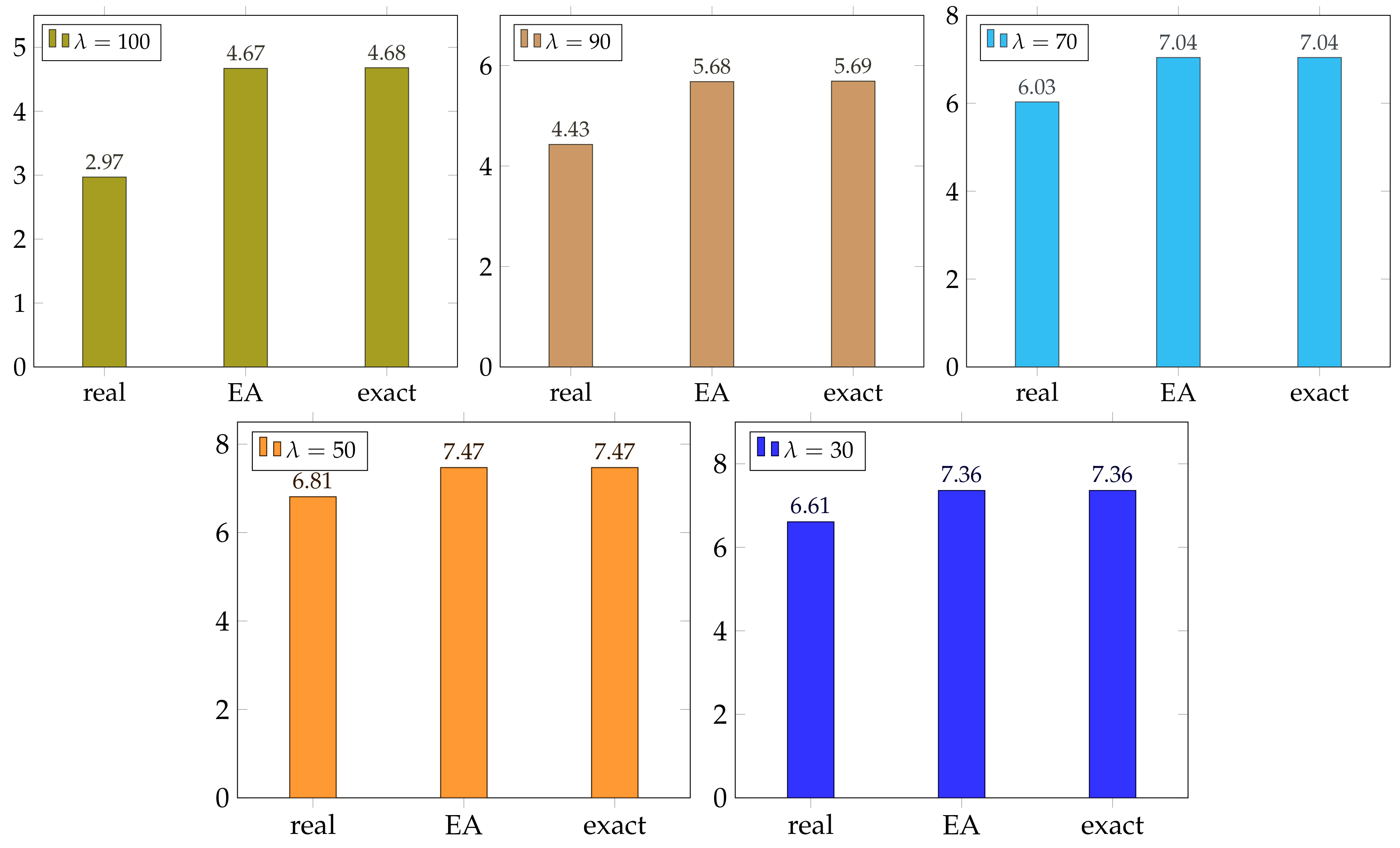
100	8.57	8.59	6.61	1.30	1.30	1.96	1.98

reports the average objective values (normalized by the number of transfer zones) for all scenarios, grouped by tolerance. Results show that both EA and the exact methods significantly improve over the baseline real solution. For BSP variant #1, the largest difference is 1.72 (4.68 – 2.97) between the exact approach and the real solution, when low user tolerance is considered ($\lambda$ = 30). Similar to the results reported in Table 5, the graphic demonstrates that improvements of the optimization methods are better in tighter BSP instances. For BSP variant #2, the best improvement of the exact method was 4.45, and the best improvement of EA was 4.45, both when $\lambda$ = 30. Results are graphically presented in Figure 7 for BSP variant #1.

Three quality of service metrics (r, $l_s$, and $l_n$) are considered in the results reported for the computed solutions in

Table 10. Average synchronizations for the studied methods.

Problem Variant #1
m	$\mathit{\lambda }$	Real		EA		Exact
	$\mathit{r}$	${\mathit{l}}_{\mathit{s}}$/${\mathit{l}}_{\mathit{n}}$	$\mathit{r}$	${\mathit{l}}_{\mathit{s}}$/${\mathit{l}}_{\mathit{n}}$	$\mathit{r}$	${\mathit{l}}_{\mathit{s}}$/${\mathit{l}}_{\mathit{n}}$
30	100	0.45	22/0	0.44	22/0	0.44	22/0
30	90	0.47	21/1	0.46	22/0	0.47	22/0
30	70	0.59	19/3	0.54	21/1	0.53	22/0
30	50	0.85	12/10	0.76	16/6	0.75	18/4
30	30	1.33	3/19	1.15	10/12	1.12	11/11
70	100	0.46	39/0	0.44	39/0	0.44	39/0
70	90	0.47	39/0	0.46	39/0	0.47	39/0
70	70	0.59	33/6	0.54	39/0	0.52	39/0
70	50	0.85	24/14	0.74	30/9	0.73	32/6
70	30	1.35	5/33	1.14	18/21	1.14	20/19
110	100	0.48	49/0	0.45	49/0	0.45	49/0
110	90	0.49	47/2	0.48	49/0	0.46	49/0
110	70	0.61	40/9	0.57	43/6	0.53	49/0
110	50	0.87	28/20	0.74	33/16	0.72	40/9
110	30	1.38	7/42	1.14	21/28	1.10	24/23
Problem Variant #2
$\mathit{m}$	$\mathit{\lambda }$	Real		EA		Exact
	$\mathit{r}$	${\mathit{l}}_{\mathit{s}}$/${\mathit{l}}_{\mathit{n}}$	$\mathit{r}$	${\mathit{l}}_{\mathit{s}}$/${\mathit{l}}_{\mathit{n}}$	$\mathit{r}$	${\mathit{l}}_{\mathit{s}}$/${\mathit{l}}_{\mathit{n}}$
30	100	0.45	22/0	0.44	22/0	0.44	22/0
30	90	0.47	22/0	0.46	22/0	0.47	22/0
30	70	0.59	22/0	0.54	22/0	0.53	22/0
30	50	0.85	16/6	0.76	19/3	0.75	19/3
30	30	1.33	3/19	1.15	5/16	1.12	7/15
70	100	0.46	39/0	0.44	39/0	0.44	39/0
70	90	0.47	39/0	0.46	39/0	0.47	39/0
70	70	0.59	38/1	0.54	39/0	0.52	39/0
70	50	0.85	28/10	0.74	35/3	0.73	35/4
70	30	1.35	5/33	1.14	18/21	1.14	20/19
110	100	0.48	49/0	0.45	49/0	0.45	49/0
110	90	0.49	49/0	0.48	49/0	0.46	49/0
110	70	0.61	46/2	0.57	48/1	0.53	49/0
110	50	0.87	34/14	0.74	41/8	0.72	44/5
110	30	1.38	7/42	1.14	21/28	1.10	22/27

, grouped by dimension (NP) and tolerance ($\lambda$). Metric r is the ratio between the average waiting time computed by the proposed timetable schedules and the threshold value that passengers are willing to wait for a transfer in each transfer zone ($W_b^{ij}$). The r metric evaluates the number of successful synchronized trips, which are represented by $r\le 1.0$, whereas unsuccessful synchronizations are represented by $r>1.0$. Metric r also allows evaluating how far from acceptable (i.e., synchronized) the trips of two lines are, considering the deviation from the ratio defined by the threshold value passengers are willing to wait (1.0). In turn, metric $l_s$ is the average number of successfully synchronized lines, whereas metric $l_n$ is the average number of not synchronized lines. All metrics are reported for each instance class regarding dimension and tolerance.

Results in Table 10 indicate that both studied optimization methods significantly improved the quality of service when compared with the real solution. Both the exact method and the EA computed lower values of the waiting time metric for all instance classes. The best improvements of the studied methods over the baseline real solution occurred for problem instances with NP = 70/110 and $\lambda$ = 30, where both exact and EA computed solutions with a higher number of synchronized lines. In turn, the largest number of synchronized lines were computed by the exact method in problem instances with NP = 110 and $\lambda$ = 30. Furthermore, better waiting time values were obtained by both exact and EA in problem instances with lower waiting time tolerance from users, with respect to the baseline real solution.

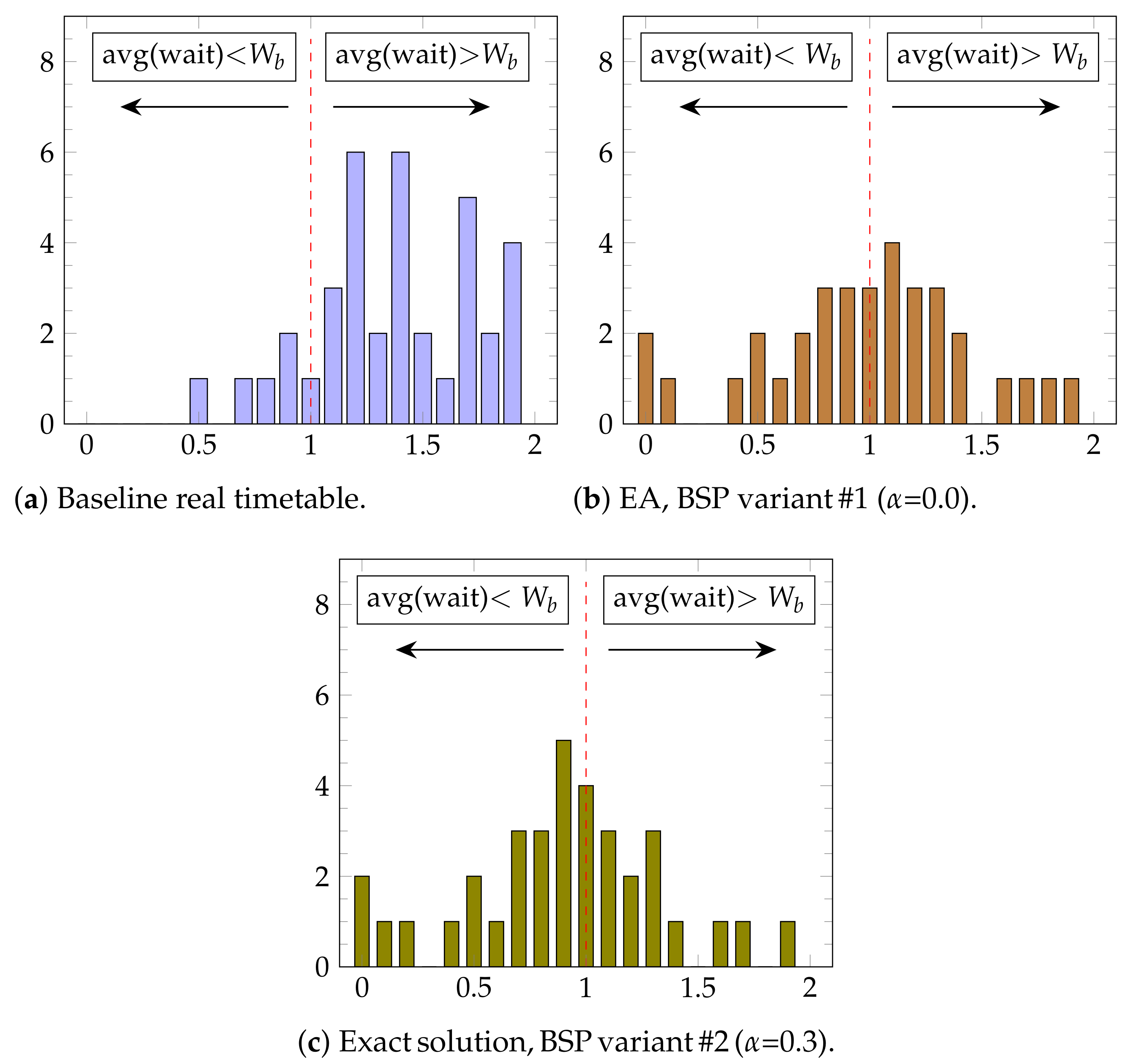
A comparison of waiting time values for transfers of all lines (normalized by $W_b$) is presented in the histograms in Figure 8. Results correspond to scenario 70.63.30.2, which is representative of the results computed for other studied BSP instances. Normalized average waiting time results are reported for the baseline real solution, the EA solution for BSP variant #1 ($\alpha$ = 0.0), and the exact solution for BSP variant #2 ($\alpha$ = 0.3). Values of the normalized average waiting time over 1.0 mean that for a number of lines in the reported scenario, the optimization methods were not able to find a combination of offset and headway values that allows lowering the waiting time for transfers under $W_b$. This occurs as a direct consequence of the inter-related design of bus lines and the behavior of passengers in each scenario, since when adjusting offsets and headways to achieve successful transfers between line i and line j in transfer zone b (i.e., for those transfers avg(wait) < $W_b$), those lines are not synchronized (at least for some trips) with other lines on other transfer zones $b*$ (i.e., for those transfers, avg(wait) > $W_{b*}$). The histograms in Figure 8 report both successful synchronizations (avg(wait) < $W_b$, on the left side of each histogram) and non-successful synchronizations (avg(wait) > $W_b$, on the right side of each histogram).

Results reported in the histograms in Figure 8 demonstrate that the exact solution effectively reduces the waiting time for a significant percentage of lines in the studied instance. The exact solution has more lines with an average waiting time lower or equal to 1 (i.e., 23 in the exact solution vs. only 6 in the real solution). Furthermore, five lines in the exact solution have an average waiting time less than 0.5 of $W_b$, whereas there is none in the real solution. Regarding larger waiting times, only 3 lines in the exact solution have more than 1.5 of the maximum value for a successful synchronization, whereas in 13 lines of the real solution, passengers must wait 1.5 more than expected to perform a multi-leg trip. The comparative results demonstrate that the solution found by the exact method synchronizes a larger number of lines, thus improving the QoS. Solutions computed by the proposed EA have a similar behavior regarding waiting times, as reported in Table 10. Similar results were obtained for other studied BSP instances, and even better results were achieved in the most restrictive instances ($\lambda =30$).

Finally, regarding execution time, both the exact and evolutionary approaches were able to compute accurate solutions in very short execution times. For problem variant #1, the execution times were less than 10 seconds. For problem variant #2, the time limit of the exact method was two hours, and the EA found the best solutions in less than five minutes.

7. Concluding Remarks

This article studied the bus timetabling synchronization problem. The problem model extends existing ones by defining extended transfer zones for every pair of bus stops. In turn, an improved model was included to account for the transfer demands of passengers, and two variants of the problem were addressed: optimizing the offset for each line, and optimizing the offset and headways for each line. For the second problem variant, the optimization domain was restricted to a certain deviation on the real headways defined for the case study to provide a proper quality of service to users.

An exact MILP approach and an EA were proposed to solve the problem. Both methods were evaluated for a real case study for the public transportation system in Montevideo, Uruguay. A total number of 75 scenarios were defined using real data about lines, headways, and transfer demands, gathered from the intelligent transportation system of Montevideo. Results were compared with the real timetable currently implemented by the city administration.

The empirical evaluation indicated that both proposed methods are able to compute solutions that are significantly improved over the real current timetable in Montevideo. The exact method computed the optimal solution for all instances in problem variant #1, improving successful synchronizations up to 66.6% (24.6% on average) over the real timetable. The EA was highly efficient for this problem variant, too, improving the synchronizations up to 66.3% (24.5% on average) over the current timetable. Problem variant #2 poses a significantly harder challenge for optimization, as the number of variables significantly increases for each considered scenario. Despite this, the exact method was able to compute an accurate solution, which provides significant improvements on the number of successfully synchronized trips over the real timetable. Improvements up to 179.9% (66.2% on average) for the exact methods and up to 174.8% (66.2% on average) for the EA. The proposed optimization methods also improved relevant quality of service metrics, such as the average waiting times for transfers, especially in tight problem instances, which reduced up to 57.8% for BSP variant #1 and up to 158.3% for BSP variant #2.

Both methods were efficient regarding computing times. The exact method provided accurate objective function values within less than a second for problem variant #1. In turn, the proposed EA is useful for solving larger problem instances of problem variant #2 in reduced execution times.

Future lines of research are related to addressing other BSP variants, e.g., explicitly focusing on the perceived waiting times for users, and modeling the real demand for direct trips from real data on ticket sales provided by the transportation system. Multi-objective versions of the problem can be devised, too, by including the explicit optimization of other relevant functions, such as the operation cost of the bus fleet and other quality of service metrics.

References

- Grava, S. Urban Transportation Systems; McGraw-Hill: New York, NY, USA, 2002. [Google Scholar]
- Nesmachnow, S.; Baña, S.; Massobrio, R. A distributed platform for big data analysis in smart cities: Combining Intelligent Transportation Systems and socioeconomic data for Montevideo, Uruguay. EAI Endorsed Trans. Smart Cities 2017, 2, 1–18. [Google Scholar] [CrossRef] [Green Version]
- Ceder, A.; Wilson, N. Bus network design. Transp. Res. Part B Methodol. 1986, 20, 331–344. [Google Scholar] [CrossRef]
- Hipogrosso, S.; Nesmachnow, S. Analysis of Sustainable Public Transportation and Mobility Recommendations for Montevideo and Parque Rodó Neighborhood. Smart Cities 2020, 3, 479–510. [Google Scholar] [CrossRef]
- Ceder, A.; Tal, O. Timetable Synchronization for Buses. In Lecture Notes in Economics and Mathematical Systems; Springer: Berlin/Heidelberg, Germany, 1999; pp. 245–258. [Google Scholar]
- Risso, C.; Nesmachnow, S. Designing a Backbone Trunk for the Public Transportation Network in Montevideo, Uruguay. In Smart Cities; Springer: Berlin/Heidelberg, Germany, 2020; pp. 228–243. [Google Scholar]
- Massobrio, R.; Nesmachnow, S. Urban Mobility Data Analysis for Public Transportation Systems: A Case Study in Montevideo, Uruguay. Appl. Sci. 2020, 10, 5400. [Google Scholar] [CrossRef]
- Nesmachnow, S.; Muraña, J.; Risso, C. Exact and Metaheuristic Approach for Bus Timetable Synchronization to Maximize Transfers. In Smart Cities; Springer: Berlin/Heidelberg, Germany, 2021; pp. 183–198. [Google Scholar]
- Eranki, A. A Model to Create Bus Timetables to Attain Maximum Synchronization Considering Waiting Times at Transfer Stops. Master’s Thesis, University of South Florida, Tampa, FL, USA, 2004. [Google Scholar]
- Ibarra-Rojas, O.; Rios-Solis, Y. Synchronization of bus timetabling. Transp. Res. Part Methodol. 2012, 46, 599–614. [Google Scholar] [CrossRef]
- Ibarra-Rojas, O.; López-Irarragorri, F.; Rios-Solis, Y. Multiperiod Bus Timetabling. Transp. Sci. 2016, 50, 805–822. [Google Scholar] [CrossRef] [Green Version]
- Saharidis, G.; Dimitropoulos, C.; Skordilis, E. Minimizing waiting times at transitional nodes for public bus transportation in Greece. Oper. Res. 2013, 14, 341–359. [Google Scholar] [CrossRef]
- Salicrú, M.; Fleurent, C.; Armengol, J. Timetable-based operation in urban transport: Run-time optimisation and improvements in the operating process. Transp. Res. Part A Policy Pract. 2011, 45, 721–740. [Google Scholar] [CrossRef]
- Daduna, J.; Voß, S. Practical Experiences in Schedule Synchronization. In Lecture Notes in Economics and Mathematical Systems; Springer: Berlin/Heidelberg, Germany, 1995; Volume 430, pp. 39–55. [Google Scholar]
- Ceder, A.; Golany, B.; Tal, O. Creating bus timetables with maximal synchronization. Transp. Res. Part Policy Pract. 2001, 35, 913–928. [Google Scholar] [CrossRef]
- Fleurent, C.; Lessard, R.; Séguin, L. Transit timetable synchronization: Evaluation and optimization. In Proceedings of the 9th International Conference on Computer-aided Scheduling of Public Transport, San Diego, CA, USA, 9–11 August 2004. [Google Scholar]
- Shafahi, Y.; Khani, A. A practical model for transfer optimization in a transit network: Model formulations and solutions. Transp. Res. Part A Policy Pract. 2010, 44, 377–389. [Google Scholar] [CrossRef]
- Abdolmaleki, M.; Masoud, N.; Yin, Y. Transit timetable synchronization for transfer time minimization. Transp. Res. Part B Methodol. 2020, 131, 143–159. [Google Scholar] [CrossRef]
- Nesmachnow, S.; Muraña, J.; Goñi, G.; Massobrio, R.; Tchernykh, A. Evolutionary Approach for Bus Synchronization. In High Performance Computing; Springer: Berlin/Heidelberg, Germany, 2020; pp. 320–336. [Google Scholar]
- Bäck, T.; Fogel, D.; Michalewicz, Z. (Eds.) Handbook of Evolutionary Computation; Oxford University Press: Oxford, UK, 1997. [Google Scholar]
- Massobrio, R.; Nesmachnow, S. Urban Data Analysis for the Public Transportation System of Montevideo, Uruguay. In Smart Cities; Springer: Cham, Switzerland, 2020; pp. 199–214. [Google Scholar]
- Nesmachnow, S.; Iturriaga, S. Cluster-UY: Collaborative Scientific High Performance Computing in Uruguay. In Communications in Computer and Information Science; Springer: Berlin/Heidelberg, Germany, 2019; pp. 188–202. [Google Scholar]
Figure 1.
The considered model for the BSP with expanded transfer zones [blue circle].
Figure 2.
Graphical representation of BSP variant #1. The offset (in blue) is the control variable, and subsequent departures are separated by a fixed time .
Figure 3.
Graphical representation of BSP variant #2. The offset () and headways () (in blue) are the control variables, and departures are separated by variable headway values.
Figure 4.
Solution representation for BSP variant #1.
Figure 5.
Solution representation for BSP variant #2.
Figure 6.
Boxplot analysis of parameter configurations for a representative BSP instance.
Figure 7.
Comparison of normalized objective function values, grouped by tolerance, for BSP variant #1.
Figure 8.
Comparative results of waiting times for the real solution, EA for BSP variant #2 ( = 0.0), and exact solution for BSP variant #2 ( = 0.3) in scenario 70.63.100.2.