Analysis of the Main Anthropogenic Sources’ Contribution to Pollutant Emissions in the Lazio Region, Italy

Abstract

Most cities worldwide suffer from serious air-quality problems, which have received increasing attention in the past decade. The most probable reason for the air-quality problems is the urban population growth, combined with a change in land use due to increasing urban areas. The emission of air pollutants is caused by different anthropogenic processes which can be categorized into the sources of urban traffic, industry, and domestic heating. Dispersion and dilution of air pollutants are strongly influenced by meteorological conditions, especially by wind direction, wind speed, turbulence, and atmospheric stability. With an increasing number of people living in cities, there is the need to examine the correlation between air pollution, local climate, and the effects these changes have on global climate. New interdisciplinary research studies are needed to increase our understanding of the interactions among these aspects. The aim is to analyze the pollutant condition in Rome and the other provinces of the Lazio region with qualitative and quantitative analysis, in order to understand which are the main pollutant sources and what is the correlation of habits of the population on air pollutant emissions.

1. Introduction

Anthropogenic atmospheric pollution is thought to be a recent problem, but it isn’t. The first records about it can be found in Ancient Rome, where a great amount of wood was used to build, cooking and heat. Some businesses in Rome needed a lot of biomass fuel (like wood, vegetal materials, or animal dung) to make the bricks and roofing tiles that were used to create Rome as well as to build the massive and majestic edifices that the city was known for. In AD 61, Lucius Annaeus Seneca, the Younger, marveled: “As soon as I had gotten out of the heavy air of Rome, from the stink of the chimneys and the pestilence, vapors, and soot of the air, I felt an alteration to my disposition.” While some individuals may have been exposed to irritating volatile organic mixtures from rotting garbage, contaminated indoor air was the cause for a large portion of the illness attributed to ambient factors in ancient times.

The Industrial Revolution made this problem bigger, and nowadays, domestic heating, road traffic, and factories are the main causes of air toxicity that can negatively affect human health [1]. IARC, International Agency for the Research of Cancer, focuses its studies on the particulate matter effects on human beings. PM_2.5, the particulate matter with particles smaller than 2.5 microns, is used as an indicator of air quality [2,3]. It is estimated that in 2010 3.2 million died because of PM_2.5. East Asia and India are the zones in which the majority of these people died [4,5].

Apart from the damages for people, pollutants can damage monuments, because of the presence of particulate matter, Nitrogen dioxide, and Sulphur dioxide [6,7,8,9]. The increase of buildings changed the parameters of temperature, humidity, wind speed, and direction in big cities [10]. This condition led to the phenomenon known as urban heat island: the heat dispersion is partially inhibited and it causes a rise in temperature compared to rural areas [11,12]. The more the pollutants stay on the street level, the more people are affected. A lot of studies were carried out to analyze the relationship between the presence of an urban canyon and the increase of the pollutant concentration [13,14,15,16,17]. Usually, the ratio between buildings height and street width is high, so the pollutant can’t disperse into the air and it remains inside urban canyon [18].

In recent years, many studies were focused on the investigation of the spatial and temporal distribution of pollutant levels in cities. The Geographic Information System (GIS) is important for scientifically portraying different elements of pollution sources and their influence on human health. Geostatistics is a widely used method for resolving problems involving the geographical and temporal distribution of parameters. Using the autocorrelation approach, Sarangi et al. [19] explored geostatistical techniques to interpolate unsampled sites. Fuentea et al. [20] conducted a similar study in which they extensively used interpolation methods to map the impacts of air pollution deterioration using chosen sample locations. The use of interpolation techniques to establish various air quality metrics is of worldwide relevance [21,22], and it is used in most metropolitan areas to analyze their spatial distributions. Whitworth et al. [23] utilized this approach to analyze benzene levels in a densely populated metropolitan area. ArcGIS tool is often used to assess geographic correlations of pollutant point sources [24,25]. A Geographic Information System is used also to highlight the land status that can be related to the pollutant level of an area. Shulgan et al. [26], analyzed the natural and agricultural regions using mathematical modeling and suggesting an automated zoning technique. Demetriou [27] uses an advanced spatial method composed of multiple regression analysis (MRA) and geographically weighted regression (GWR). Kwiecień and Szopińska [28] used geostatistical modeling to assess the size of a risk area to the CO levels exposure produced by traffic.

The study of the pollutant level of an urban area has growing importance due to developing air pollutant prevention and environmental management [29]. In this context, the prediction of the air pollutant level has received great attention by recent research [30,31,32,33]. Numerical prediction methods are widely used to predict the pollutant level in cities [34,35,36]. Cordano and Frieze [37] used a deterministic model, Tian and Chen [38] used an empirical black-box model, Russell et al. [39] use a statistical model while Suleiman et al. [40] adopt a machine learning model. However, the difference in regional conditions in terms of geography characteristics, climatic conditions, economy, population, and industrial layout, as well as the chemical complexity of air pollutants have raised the management and prediction challenges [41,42]. For this reason, trying to understand the emission features with a spatial and temporal distribution point of view in cities and regions can contribute to the development of policy and environmental strategies in order to reduce the air pollutant level.

In Italy, often the policy and environmental strategies aimed to reduce the pollutant concentrations were taken in the same way for the whole country. In many cases to the variation of the characteristics of the sites as listed in the preceding paragraph, can induce a different pollutant condition that needs different types of policy directive to decrease the urban pollutant levels. Due to the extreme variability of the geography, climatic, population density, industrial structures conditions in the Lazio region and at the same time inside the Rome city, which is very vast and has different types of build-up, greening, and traffic conditions, finding a pollutant level correlation can help environmental management of each area.

The aim of this study is to find a correlation of pollutant concentration between the different sites of the Lazio region which is in the middle of Italy and in which there is located the capital Rome, one of the largest cities in the world. Experimental data were taken from 39 monitoring stations considering the pollutant concentrations of [CO], [SO₂], [NO_X], [NO], [NO₂], [C₆H₆], [PM₁₀], [PM_2.5] and [O₃]. At the same time, it was investigated the possible main pollutant sources for the Lazio region in order to focus on the priority of future policy strategies. In this way, a nowadays strategy in Italy was analyzed in order to verify the validity of this technique from a pollutant level decrease point of view.

2. Materials and Methods

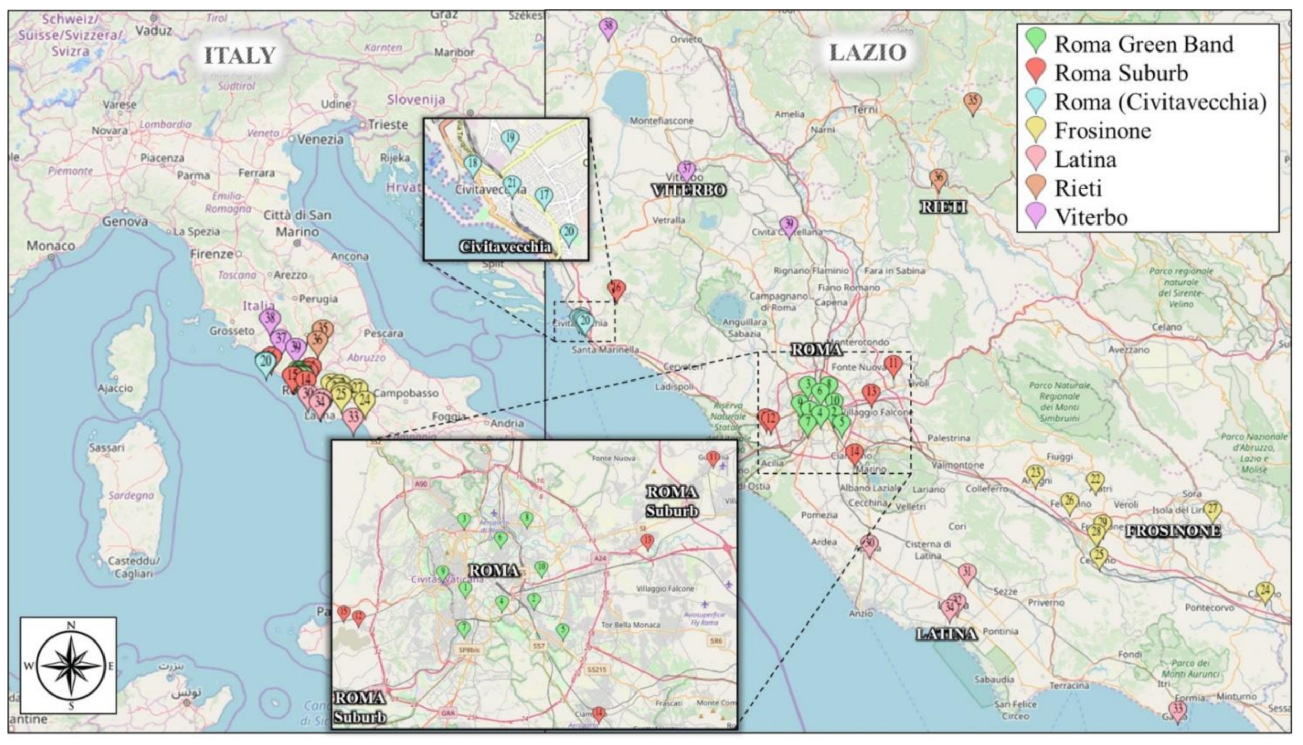
2.1. Characteristics of the Study Area

Rome is the capital of Italy and one of the most overcrowded cities of Europe (3 million people for 12,850 km²). Considering the extra-urban areas, people are more than four million. It is a historical city that traces its origin to 753 a.C. and it was the capital of the biggest empire ever. That’s why it is known as the eternal city and its cultural heritage finds no equals. Thanks to its position, Rome shows a Mediterranean climate: temperate winter and hot summer, with temperatures from 0 to 36. The greatest problem of this city is the lack of an adequate net of public transport, so people use cars [43]. Apart from traffic, there are a lot of other pollutant activities, such as domestic heating.

2.2. Monitoring Station Network

ARPA Lazio is the agency that monitors the air condition in the region of Lazio [44]. The monitoring network used in the present work consists of 39 monitoring stations of [CO], [SO₂], [NO_X], [NO], [NO₂], [C₆H₆], [PM₁₀], [PM_2.5], and [O₃] that are shown in Figure 1 and listed in

Table 1. Pollutant monitoring stations of Rome center and suburbs used in the present study.

Area	Name	Number	Background
Roma Green Band	Arenula	1	Low Traffic
	Preneste	2	Low Traffic
	Francia	3	High Traffic
	Magna Grecia	4	High Traffic
	Cinecittà	5	Low Traffic
	Villa Ada	6	Low Traffic
	Fermi	7	High Traffic
	Bufalotta	8	Low Traffic
	Cipro	9	Low Traffic
	Tiburtina	10	High Traffic
Roma Suburb	Guidonia	11	Industrial
	Castel di Guido	12	Rural Area
	Cavaliere	13	Rural Area
	Ciampino	14	Industrial
	Malagrotta	15	Low Traffic
	Allumiere	16	Rural Area
Roma (Civitavecchia)	Civitavecchia	17	High Traffic and Industrial
	Porto	18	High Traffic and Industrial
	Villa Albani	19	High Traffic and Industrial
	Via Morandi	20	High Traffic and Industrial
	Via Roma	21	High Traffic and Industrial

and

Table 2. Pollutant monitoring stations of the Lazio region province were used in the present study.

Area	Name	Number	Background
Frosinone	Alatri	22	High Traffic and Industrial
	Anagni	23	High Traffic and Industrial
	Cassino	24	High Traffic and Industrial
	Ceccano	25	High Traffic and Industrial
	Ferentino	26	High Traffic and Industrial
	Fontechiari	27	Rural Area
	Frosinone-Scalo	28	High Traffic and Industrial
	Mazzini	29	High Traffic and Industrial
Latina	Aprilia2	30	Low Traffic
	Latina-Scalo	31	Low Traffic
	Via Tasso	32	Low Traffic
	Gaeta	33	Medium Traffic and Industrial
	Viale de Chirico	34	Low Traffic
Rieti	Leonessa	35	Rural Area
	Rieti 1	36	Medium Traffic
Viterbo	Viterbo	37	Medium Traffic
	Acquapendente	38	Rural Area
	Civita Castellana	39	Medium Traffic and Industrial

. The monitoring stations are located in strategic places. It collects data hour by hour in a place with a great concentration of pollution. Ten monitoring stations are used to evaluate the pollutant conditions inside the city of Rome (called “Roma Green Band”), while other 6 stations are used to evaluate the pollutant concentrations near the city (called “Roma Suburb”). Civitavecchia is monitored by another station set because it’s very far from Rome, even if it is in its province (called “Roma (Civitavecchia)”).

In Table 1 and Table 2, the stations used in the present work are listed. The tables show the background of each station. They are useful to impute the pollutant concentrations to the urban traffic, industrial or building heating.

2.3. Pollutant Legislation

In the 1960s, the USA made the first laws to guarantee air quality. In Italy, it is regulated by DPR 203/88 [45], which states that it’s possible to define as pollution each element able to:

• Alter the normal environmental condition and air quality;
• Generate a danger for human health;
• Compromise the environment;
• Alter the biological resources and public and private goods.

In this perspective, the 2008/50/CE directive of the European Parliament [46] finds its application in Italy through D.Lgs. 155\2010 [47], which defines the pollutant agents, the concentration limits into the air, the laws, and the measures able to reduce the pollutant concentrations. Benzene, carbon monoxide, nitrogen oxides, ozone, PM_2.5, PM_10, and sulfur dioxide are defined as pollutants. For each of them was defined a limit to reducing its effect.

Table 3. Directive 2008/50/EC standards of the main pollutant.

Pollutant	Concentration	Averaging Period	Permitted Excess Each Year
PM10	50 µg/m3	24 h	35
PM10	40 µg/m3	1 year	-
PM2.5	25 µg/m3	1 year	-
NO2	200 µg/m3	1 h	18
NO2	40 µg/m3	1 year	-
SO2	350 µg/m3	1 h	24
SO2	125 µg/m3	24 h	3
O3	120 µg/m3	Maximum daily 8 h mean	25 days averaged over 3 years
CO	10 mg/m3	Maximum daily 8 h mean	-
C6H6	5 µg/m3	1 year	-

reports the most relevant pollutants for this study.

2.4. Type of Pollutant

Carbon monoxide (CO) [48] is a colorless, odorless gas emitted from combustion processes. Nationally and particularly in urban areas the, majority of CO emissions to ambient air come from mobile sources. CO can cause harmful health effects by reducing oxygen delivery to the body’s organs (like heart and brain) and tissues. At extremely high levels, CO can cause death.

Nitrogen dioxide (NO₂) [48] is one of a group of highly reactive gasses known as “oxides of nitrogen,” or “nitrogen oxides (NO_X).” NO₂ is used as the indicator for the larger group of nitrogen oxides. NO₂ comes from emissions by cars, trucks and buses, power plants, and off-road equipment. In addition to contributing to the formation of ground-level ozone, and fine particle pollution, NO₂ is linked with a number of adverse effects on the respiratory system.

Sulfur dioxide (SO₂) [48] is one of a group of highly reactive gasses known as “oxides of sulfur.” The largest sources of SO₂ emissions are from fossil fuel combustion at power plants (73%) and other industrial facilities (20%). SO₂ is linked with a number of adverse effects on the respiratory system.

Particulate matter (PM) [48] is a complex mixture of extremely small particles and liquid droplets. Particle pollution is made up of a number of components, including acids (such as nitrates and sulfates), organic chemicals, metals, and soil or dust particles. The size of particles is directly related to their potential for causing health problems. Once inhaled, these particles can affect the heart and lungs and cause serious health effects. There are two categories of PM:

• “Inhalable coarse particles,” such as those found near roadways and dusty industries, are larger than 2.5 micrometers and smaller than 10 micrometers in diameter.
• “Fine particles,” such as those found in smoke and haze, are 2.5 micrometers in diameter and smaller. These particles can be emitted from sources such as forest fires, or they can form when gases emitted from power plants, industries and automobiles react in the air.

With reference to NO₂, SO_2, and (PMs) there is general agreement in the scientific literature that they are the main agent responsible for the damage encountered on monuments and historical buildings in urban areas [34]. Atmospheric composition is of unquestionable importance in the study of the damage produced on building materials of artistic interest since it directly influences the species characteristics and entity of the degradation mechanism occurring on the cultural heritage.

Ozone (O₃) [48] is not emitted directly into the air, but it is created by chemical reactions between oxides of nitrogen (NO_X) and volatile organic compounds (VOC) in the presence of sunlight. Emissions from industrial facilities and electric utilities, motor vehicle exhaust, gasoline vapors, and chemical solvents are some of the major sources of NOx and VOC. Breathing ozone can trigger a variety of health problems, particularly for children, elderly people, and people of all ages who have lung diseases such as asthma. Ground-level ozone can also have harmful effects on sensitive vegetation and ecosystems.

Benzene (C₆H₆) [48] is used as a constituent in motor fuel; as a solvent for fats, waxes, resins, oils, inks, paints, plastics, and rubber, in the extraction of oils from seeds and nuts, and in photogravure printing. It is also used as a chemical intermediate and in the manufacture of detergents, explosives, pharmaceuticals, and dyestuffs. It is found in the air from emissions from burning coal and oil, gasoline service stations, and motor vehicle exhaust. Acute (short-term) inhalation exposure of humans to benzene may cause drowsiness, dizziness, headaches, as well as eye, skin, and respiratory tract irritation, and, at high levels, unconsciousness. Chronic (long-term) inhalation exposure has caused several blood disorders, including reduced numbers of red blood cells and aplastic anemia, in occupational settings. Negative effects on reproduction have been reported for women exposed to high levels of inhalation, and adverse effects on the developing fetus have been observed in animal tests. Increased incidence of leukemia (cancer of the tissues that form white blood cells) has been observed in humans occupationally exposed to benzene.

2.5. Anthropogenic Sources

Today, air quality affects even small cities. To know the values of the emissions is fundamental to monitor air quality and consequently to find solutions to it.

Pollutant emissions can be divided into localized and spread. The first are the ones that can be studied singularly and can be localized. They show emissions higher than 90–100 tons per year that are referred to industries that use combustion processes. The second are the ones that can’t be classified as the first ones and they don’t go over the limits of the localized ones. They are referred to as urban traffic and building heating systems [44].

Cars are one of the main reasons for the increase in cities pollution. In recent years, the percentage of goods and people on the road increased compared to railway transportation. In Italy, in the 1980s there were about 20 million vehicles, in the 1990s there were about 33 million of them. This value became 39 million in 1998 [49]. Referring to the total amount of emission of road traffic, urban traffic represents 77% of the CO, 39% of CO₂, 27% of NO_X, and 29% of particulate matter [50].

Together with road traffic, building heating systems are an important factor for the air quality standard. They aren’t regulated yet, so they are difficult to monitor and improve.

The production of a pollutant that can be found in the air is caused both by natural processes, like volcanos activities and by human production. The natural processes are not taken into account in this study because they produce fewer effects than the anthropogenic ones, which include industrial processes, heating systems, energy generators, urban traffic, and even smoke. That’s why urban and industrial areas are more exposed than rural ones and show a higher level of risk. Anyway, the city of Rome is taken into account only the effects of urban traffic and heating systems.

2.5.1. Urban Traffic

Urban traffic is tough to be the main cause of pollution in the city of Rome because of the emission of incomplete combustion.

Most of the cars are petrol or diesel, and there is a very low increase in the use of electric or hybrid engines. In 2015, for 4,340,474 people, there were 2,665,174 cars, 521,070 motorcycles and 8589 buses [51]. Because of their incomplete combustion, diesel engines produce pollutants. The most relevant are sulfur dioxide (SO₂), carbon monoxide (CO) nitrogen oxides (NO_X), and particulate matter, which is the one to pay more attention to.

The benzene (C₆H₆) is used as a constituent in motor petrol and it causes the formation of toxic substances like carbon monoxide (CO), nitrogen oxides (NO_X), and particulate matter.

2.5.2. Heating Systems

The aim of the heating system is to make people reach their wellness with an adequate temperature. In Rome, the most used systems are the independent and centralized ones. A heating generator, powered by liquid or gas fuel (methane or gasoline), makes these systems work.

Methane is the most used gas thanks to its widespread diffusion in Italy. It is called natural gas because it is a hydrocarbon already present in nature. It’s quite cheap and it produces pollutant as CO, NO_X, PM₁₀, and PM_2.5.

Diesel boilers are safer than gas ones but they pollute more. In Italy, diesel isn’t as cheap as in the rest of Europe. They produce SO_X and SO₂.

Anyway, pollutants are produced because of the incomplete combustion that leads to the formation of CO and NO_X.

Condensing boilers are able to save energy from steam water and heat from drain gas. Fumes are made cold as steam goes into liquid losing heat that goes in the water in the thermic system. The use of it reduces the emissions of CO, CO₂ e NO, and particular matter up to 70%.

Different from urban traffic, heating systems are not regulated by any Italian or European law. The only rule is for the systems under 35 kW, which have to show less than 0.1% of CO in the drained gas. There are no limits for particular matter and NO_X so producers are not so interested in environmental safeness.

2.6. Methodology

In this paper, the correlation of pollution concentration between different types of urban context was investigated to find a possible link between pollutant level and urban context. Considering the monitoring station network shown in Figure 1, the Lazio region, like Rome, has an extreme variability of the geography, climatic, population density, industrial structures conditions. These differences should bring to a different type of policy and environmental strategies in order to reduce the pollution concentration in each site. Furthermore, the quantification of the pollutant concentration impact from different types of anthropogenic sources can help to decide the priority of future policy strategies. To accomplish the objective of the present paper there is the need to analyze the spatial and temporal dependence of pollutant concentration in the different types of locations. Therefore, the quantification of the anthropogenic sources’ contribution can be investigated. The steps followed in the present paper are:

• Spatial dependence of pollutant concentrations: The analysis considers the cross-correlation of the single pollutant concentration between the different locations. Cross-correlation is a measure of similarity of two data series as a function of the lag of one relative to the other. The aim of this analysis is to investigate the similarity of pollutant trends from different types of locations in order to find the same corporation in a different area. The final results depend on the spatial distribution of the sites taken into account and on the different seasons of the year;
• Temporally dependent on pollutant concentrations: The analysis investigates the trend of pollutant concentrations over years. The objective of this analysis is to find if there is the same behavior over time or not in depending also for the different seasons;
• Anthropogenic sources’ contribution to pollutant emissions: The analysis compares the mean pollutant concentration variation during the day for the different locations. the analysis is considered separately the contribution of the different type types of anthropogenic sources with the possibility to quantify their impact on pollutant concentration.

Furthermore, the nowadays policy strategy in Italy was analyzed in order to verify the validity of this technique from a pollutant level decrease point of view.

3. Results and Discussion

In order to analyze the emissions by heating systems and urban traffic, the data of pollutant concentration of the year were divided taking into account the periods with heating systems turned on or off. Based on DPR n.412/1993 [52], heating systems are turned on from 1 November to 15 April for 12 h per day.

3.1. Spatial Dependence of Pollutant Concentrations

The cross-correlation represents the similitude of two signals depending on a time translation of one of them. In the present study, it was used to evaluate the results from different stations. Cross-correlation of zero represents no dependence of the pollutant concentration for different monitoring stations, the value of +1 represents the same trend and the value of −1 represents an opposite trend. It is possible to consider values greater than 0.4 as representative of a good similarity of two monitoring stations or areas for a specific pollutant.

The aim of the cross-correlation analysis is to understand if pollutant monitoring stations in different areas show similar results. It is useful to consider the mean values of contaminants of each station of Roma Green Band, in order to represent the average pollutant concentrations of Rome.

Table 4. Cross-correlation values between Roma Green Band and suburbs or province stations of [C₆H₆] in 2015.

	Monitoring Station	From July to August	From April to June	From September to November	From November to April
Suburbs	Malagrotta	0.15	0.22	0.39	0.69
	Ciampino	0.54	0.56	0.53	0.65
Provinces	Latina	0.32	0.18	0.39	0.64
	Frosinone	0.20	0.36	0.47	0.56
	Rieti	0.13	0.22	0.46	0.41
	Viterbo	0.50	0.47	0.52	0.66

,

Table 5. Cross-correlation values between Roma Green Band and suburbs or province stations of [CO] in 2015.

	Monitoring Station	From July to August	From April to June	From September to November	From November to April
Provinces	Latina	0.19	0.08	0.48	0.59
	Frosinone	0.47	0.48	0.72	0.67
	Rieti	0.19	0.43	0.57	0.46
	Viterbo	0.24	0.47	0.57	0.53
	Civitavecchia	0.30	0.46	0.51	0.53

,

Table 6. Cross-correlation values between Roma Green Band and suburbs or province stations of [NO_X] in 2015.

	Monitoring Station	From July to August	From April to June	From September to November	From November to April
Suburbs	Guidonia	0.48	0.60	0.72	0.82
	C. di Guido	0.61	0.66	0.50	0.56
	Cavaliere	0.64	0.64	0.72	0.72
	Ciampino	0.56	0.54	0.47	0.56
	Malagrotta	0.69	0.73	0.67	0.77
	Allumiere	0.19	0.28	0.15	0.27
Provinces	Latina	0.64	0.66	0.72	0.78
	Frosinone	0.73	0.71	0.76	0.80
	Rieti	0.53	0.59	0.59	0.63
	Viterbo	0.47	0.47	0.69	0.71
	Civitavecchia	0.43	0.35	0.52	0.59

,

Table 7. Cross-correlation values between Roma Green Band and suburbs or province stations of [NO₂] in 2015.

	Monitoring Station	From July to August	From April to June	From September to November	From November to April
Suburbs	Guidonia	0.48	0.55	0.67	0.75
	C. di Guido	0.57	0.60	0.45	0.55
	Cavaliere	0.66	0.66	0.69	0.77
	Ciampino	0.54	0.43	0.56	0.69
	Malagrotta	0.63	0.67	0.62	0.72
	Allumiere	0.23	0.30	0.25	0.42
Provinces	Latina	0.65	0.64	0.73	0.76
	Frosinone	0.70	0.64	0.73	0.77
	Rieti	0.45	0.48	0.62	0.70
	Viterbo	0.50	0.47	0.70	0.78
	Civitavecchia	0.52	0.43	0.49	0.65

,

Table 8. Cross-correlation values between Roma Green Band and suburbs or province stations of [NO] in 2015.

	Monitoring Station	From July to August	From April to June	From September to November	From November to April
Suburbs	Guidonia	0.48	0.65	0.71	0.81
	C. di Guido	0.63	0.63	0.40	0.39
	Cavaliere	0.61	0.63	0.69	0.67
	Ciampino	0.61	0.62	0.43	0.47
	Malagrotta	0.71	0.74	0.59	0.74
	Allumiere	0.19	0.23	0.05	0.16
Provinces	Latina	0.58	0.62	0.66	0.76
	Frosinone	0.73	0.75	0.75	0.80
	Rieti	0.60	0.70	0.49	0.56
	Viterbo	0.33	0.51	0.57	0.64
	Civitavecchia	0.26	0.37	0.54	0.55

,

Table 9. Cross-correlation values between Roma Green Band and suburbs or province stations of [O₃] in 2015.

	Monitoring Station	From July to August	From April to June	From September to November	From November to April
Suburbs	Cavaliere	0.93	0.91	0.85	0.85
	C. di Guido	0.90	0.88	0.83	0.80
	Malagrotta	0.93	0.91	0.88	0.87
	Allumiere	0.40	0.31	0.38	0.47
Provinces	Latina	0.81	0.81	0.78	0.78
	Frosinone	0.81	0.81	0.80	0.76
	Rieti	0.77	0.81	0.77	0.83
	Viterbo	0.77	0.74	0.75	0.82
	Civitavecchia	0.51	0.53	0.60	0.69

,

Table 10. Cross-correlation values between Roma Green Band and suburbs or province stations of [SO₂] in 2015.

	Monitoring Station	From July to August	From April to June	From September to November	From November to April
Suburbs	Guidonia	0.03	0.32	0.28	0.33
	Malagrotta	0.21	0.14	−0.24	0.31
	Allumiere	0.19	0.16	−0.04	−0.02
Provinces	Latina	0.20	0.11	0.19	0.16
	Frosinone	0.18	0.10	0.31	0.50
	Rieti	0.25	0.14	0.24	0.22
	Viterbo	0.17	0.14	0.23	0.13
	Civitavecchia	0.18	0.30	0.10	0.19

,

Table 11. Cross-correlation values between Roma Green Band and suburbs or province stations of [PM₁₀] in 2015.

	Monitoring Station	From July to August	From April to June	From September to November	From November to April
Suburbs	Guidonia	0.90	0.92	0.95	0.92
	C. di Guido	0.95	0.91	0.92	0.92
	Cavaliere	0.94	0.88	0.96	0.94
	Ciampino	0.90	0.90	0.93	0.82
	Malagrotta	0.90	0.69	0.93	0.93
	Allumiere	0.84	0.76	0.57	0.75
Provinces	Latina	0.92	0.90	0.92	0.90
	Frosinone	0.89	0.92	0.90	0.89
	Rieti	0.78	0.82	0.83	0.75
	Viterbo	0.84	0.91	0.93	0.88
	Civitavecchia	0.88	0.91	0.91	0.91

and

Table 12. Cross-correlation values between Roma Green Band and suburbs or province stations of [PM_2.5] in 2015.

	Monitoring Station	From July to August	From April to June	From September to November	From November to April
Suburbs	Guidonia	0.93	0.90	0.97	0.92
	C. di Guido	0.89	0.89	0.95	0.95
	Cavaliere	0.91	0.89	0.97	0.94
	Malagrotta	0.75	0.72	0.86	0.93
Provinces	Latina	0.87	0.84	0.92	0.76
	Frosinone	0.87	0.85	0.91	0.87
	Rieti	0.84	0.82	0.91	0.80
	Viterbo	0.87	0.83	0.85	0.79

show the cross-correlation results for each pollutant concentration between the mean values of the Roma Green Band and suburbs or province monitoring stations. In the tables, the values are referred to four periods of the year. “From July to August” is the summer period in which there is low urban traffic due to the summer holidays. “From April to June” and “from September to November” are periods with only urban traffic. “From November to April” is the winter period and it is influenced both by urban traffic and building heating systems.

In order to summarize the results of Table 4, Table 5, Table 6, Table 7, Table 8, Table 9, Table 10, Table 11, Table 12 and

Table 13. Cross-correlation average, maximum and minimum values between Roma Green Band and suburbs or province stations of all pollutant concentrations in 2015.

	[C6H6]	[CO]	[NOX]	[NO2]	[NO]	[O3]	[SO2]	[PM10]	[PM2.5]
Average	0.43	0.45	0.59	0.59	0.56	0.75	0.18	0.88	0.87
Maximum	0.69	0.72	0.82	0.78	0.81	0.93	0.50	0.96	0.97
Minimum	0.13	0.08	0.15	0.23	0.05	0.31	−0.24	0.57	0.72

are shown the average, maximum, and minimum cross-correlation values. Considering all the pollutant concentrations, the average value ranges from 0.18 for [SO₂] to 0.88 for [PM₁₀]. Despite the value of [SO₂] the average cross-correlation is always higher than 0.4 indicating that the pollutant concentration of Roma Green Band area with the suburbs or province ones have the same trend. This affirmation is more relevant considering [PM₁₀] and [PM_2.5] in which the cross-correlation values reach the higher values ranging from 0.57 to 0.96 and from 0.72 to 0.97 respectively. Considering the seasons, it is possible to notice that the cross-correlation values increase in the winter because of the higher use of heating systems that seems to be the main pollutant source in this period.

Regarding Sulphur dioxide, the cross-correlation reaches the minimum average value with a range from −0.24 to 0.50. in this case, the pollutant concentrations of the Roma Green Band area don’t have the same trend as the other locations. This is because there is a very low concentration magnitude of [SO₂], and it behaves as background noise.

Rural areas are usually places with a low presence of buildings and consequently, a low presence of heating systems and a low number of vehicles circulating in the area. Considering the Allumiere station, which is in a low populated area identified as a rural area of the Rome suburb, it is possible to notice that the average cross-correlation values are 0.22, 0.30, 0.16, 0.39, and 0.73 for respectively [NO_X], [NO₂], [NO], [O₃] and [PM₁₀]. Comparing those values with the ones calculated for the Castel di Guido and Cavaliere stations, which are considered as a rural area of Rome suburb as Allumiere, the cross-correlation values for the same pollutant concentrations are about 0.63, 0.62, 0.58, 0.87, and 0.93. This is an interesting result that shows how the proximity to Rome influences the levels of pollution whenever the location is a rural or urban area.

The spatial dependence analysis leads to the consideration that the pollutant concentration trend of the core of Rome city (named Roma Green Band) has the same trend to the other urban areas whenever they have low or high traffic characteristics especially regarding the particular matter ([PM₁₀] and [PM_2.5]). On the other hand, rural areas that are far from cities don’t have the same pollutant concentration behavior especially due to the low presence of traffic because, as mentioned before, the heating systems are turned on about 12 h per day during winter for the rural and urban context.

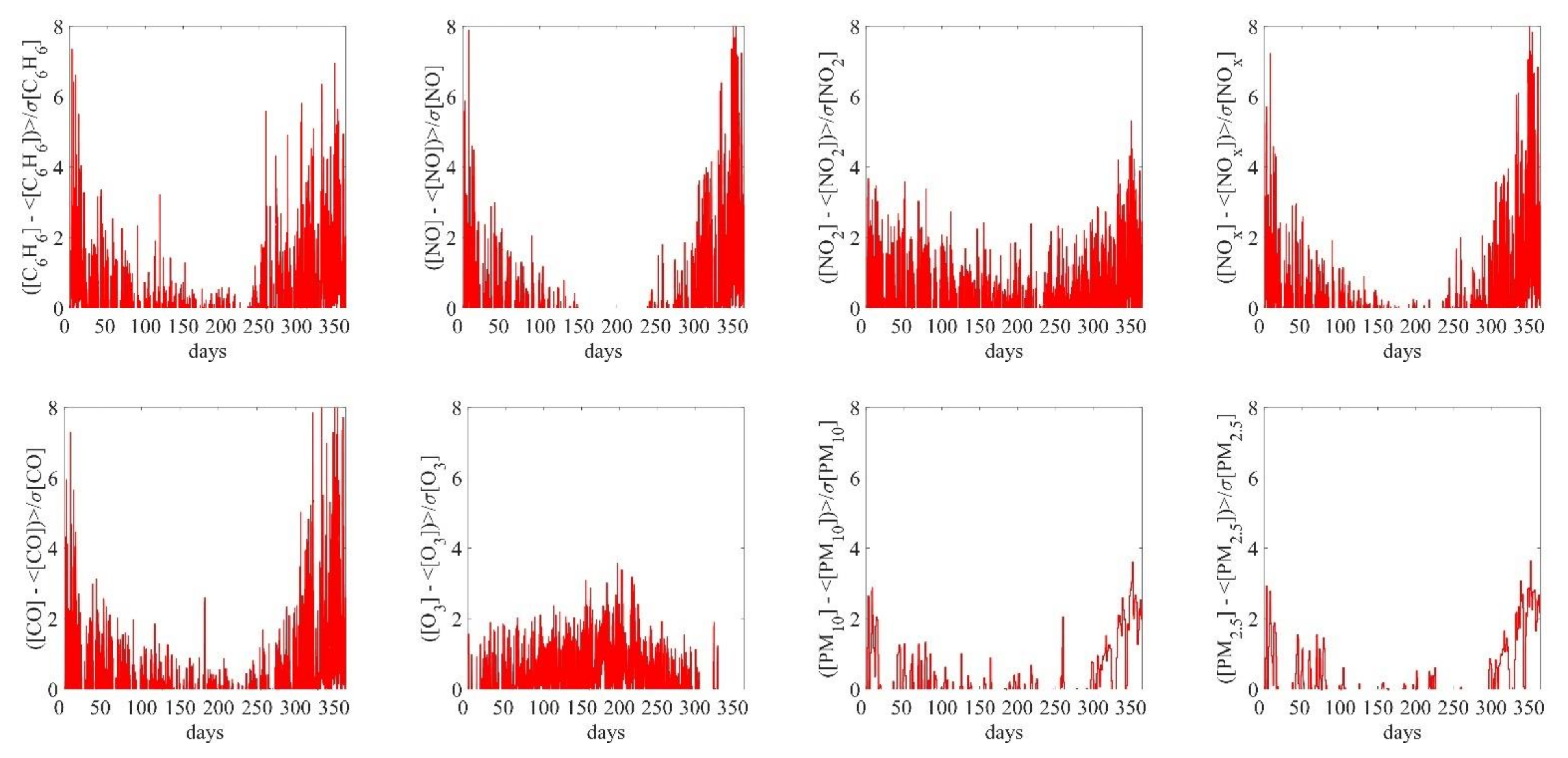
3.2. Temporally Dependence of Pollutant Concentrations

The main result of the cross-correlation analysis is that the pollutant concentration trend of Roma Green Band is the same in the other suburbs or provinces areas. For this reason, the following analysis is focused on the mean values of contaminants of each station of Roma Green Band, that will be representative of the pollutant concentrations trend in all the monitoring station of the Lazio region.

Figure 2 shows the trends from 2006 to 2015 of pollutant concentrations in Rome. In this analysis, the values of the period from July to August aren’t taken into account, because the urban traffic values are very low due to the summer holidays that lead people outside the cities. The blue line of Figure 2 identifies the average pollutant concentration in winter taking into consideration the data from November to April in which the heating systems are turned on (based on DPR n.412/1993 [52]). The red line referred to the average pollutant concentration in spring and autumn in which the heating systems are turned off (period from April to June and from September to November).

It is possible to notice that the values of most of the pollutants are decreasing in the years due to the update of the laws of pollutant emissions. Only the ozone concentration has a rising trend during the years and has a higher value in spring and autumn than in winter, because of its dependence on solar radiation. Considering the difference of winter and spring-autumn values there is an average percentage deviation of about 58.8% with a range from 20.1% to 127.4% excluding the [O₃] that have an opposite trend despite the other pollutant concentrations. This result indicates that there is an average pollutant level increase of 58.8% from spring-autumn, in which the main anthropogenic pollutant source is urban traffic, to winter where there are heating systems are turned on. This highlights the importance to take some policy strategies to decrease the pollutant emissions from heating systems.

Focusing on all the pollutant concentrations excluding the [O₃], that have an opposite trend despite them, the average difference of pollutant level year after year is about −1.6% for winter and −4.1% for spring-autumn with a range from 1.3% to −3.2% in winter and from −1.4% to −6.2% in spring-autumn. These results indicate that there is a decrease year after year of pollutant concentrations both in winter and in spring-autumn. Nevertheless, the range for spring-autumn, which is directly related to urban traffic, has only negative values (from −1.4% to −6.2%) denoting an average decrease every year after year of the pollutant concentration in these seasons. Different results are for winter in which the range has positive values (from 1.3% to −3.2%) denoting that the average decrease every year after year isn’t for all the pollutant concentrations. Focusing the attention on these aspects, the only pollutant that has an average increase year after year in winter is [PM_2.5] that has a value of 1.3%. As a matter of fact, in Figure 2 it is possible to notice that the trend line in winter is quite constant year after year despite the one of spring-autumn that decrease. Regarding the [O₃] the results are an increase of the level year after year of about 4.4% and 6.2% for winter and spring-autumn cases respectively.

The presence of heating systems turned on in winter denotes a higher pollutant emission. As a matter of fact, in Figure 2 the blue line is always over the red line despite the ozone concentration. This result affirms that the heating systems in cities have an important contribution to the pollutant level. Furthermore, the emission from these systems leads to a more irregular variation unlike in spring and autumn due to the variability of climate during the years (colder or less cold winter leads to a different use of heating systems). The higher pollutant concentration in winter than in spring and autumn is due also to the cooling air masses that promotes the stagnation at low altitude. So, the air temperature inside cities can influence the pollutant concentration at the pedestrian level. For this reason, the urban heat island phenomenon plays an important role, that is the increase of urbanization lead to the change of climatic conditions [53]. In particular, the increase of waterproof surfaces and the build-up area in cities lead to the increase of the air temperature in comparison with rural areas. High temperatures in summer improve the natural convention phenomenon that increases the mixing with clean air and the consequent dispersion of the pollutant concentration. It is important to remember that the more the pollutants stay on the street level, the more people are affected.

Focusing on 2015, to quantify the differences of urban traffic and building heating systems sources, the mean pollutant concentration of the period spring-summer-autumn, in which there is only urban traffic, was removed from the data. The results of this analysis are shown in Figure 3 in which the data set were represented in a normalized form in order to have zero mean and unitary standard deviation defined as follows:

$$\widehat{\left[x_i\right]}=\frac{\left[x_i\right]-⟨\left[x_i\right]⟩}{{\sigma }_{\left[x_i\right]}}$$

(1)

The highest values can be found in December, not only for the role of the heating systems but also for a bigger presence of traffic because of Christmas. It is useful to clarify that the values in Figure 3 are the results of the difference of the pollutant concentration in time by time with the mean values in spring, summer, and autumn in order to decurtate the pollutant level from the urban traffic sources. In this way, the values shown in Figure 3 should show only the contribution of the heating systems. Of course, the high traffic during Christmas can’t be eliminated just by the mean value of spring, summer, and autumn. So, values in Figure 3 represent the variability of the pollutant concentration compared to the traffic sources.

In most of the cases, the variability of the pollutant concentrations reaches 8σ indicating, especially during December, a high oscillation compared to the mean value during the winter season. So, the analysis on the pollutant fluctuation shown in Figure 3, that considered 2015, can be done for all the other years, considering that there is an important variation of the pollutant concentration during the year focusing most of the variability during the winter due to the turning on of heating systems and to the population actions during the year. As mentioned above, at Christmas and more generally during festivity people go out more often to buy some presents or to do the shopping at the supermarkets. In these cases, the urban traffic in cities can considerably increase with a variability calculated up to 8σ. This aspect highlights the importance to take some policy strategies that can help to control pollutant emissions, especially during the festivity.

The temporal dependence analysis leads to the consideration that the pollutant concentration in Roma Green Band, so in cities, had a decrease year after year through the update of the laws of pollutant emissions especially for vehicles, excluding the ozone that has an opposite trend. Furthermore, the presence of heating systems brings to a significant increase of the pollutant concentrations during the year with a difference from winter to spring-autumn of about 58.8%. This highlights the importance to take some policy strategies to decrease the pollutant emissions from heating systems through for example the adoption of high-efficiency thermal plants. Moreover, the analysis of the pollutant fluctuation during the year brings to the consideration to adopt policy strategy that can help to control the pollutant emissions, especially during the festivity.

3.3. Anthropogenic Sources’ Contribution to Pollutant Emissions

The average distribution of pollutants is reported in order to better understand the way of acting of the population. Figure 4 shows the day variation of pollutants in 2015, considering the mean value hour per hour and from winter to spring-autumn. The higher values can be traced in two times related to a greater flow of cars, when people go out in the morning and when they come back home in the evening (9.00 a.m., 7 p.m.). At night, there are lower values due to the turned-off heating systems (an Italian habit). In the winter, the values are even higher because of the heating systems.

It is worth noticing that Frosinone shows, for most pollutant concentrations, higher values than Rome. It is peculiar because Rome is greater than Frosinone. These results are due to the vast presence of industrial plants in the area near Frosinone.

Starting with the assumption that the pollutant concentration in winter is the combination of building heating systems and urban traffic while in spring and autumn the pollutant concentration is due only to urban traffic, in Table 5, Table 6, Table 7, Table 8, Table 9, Table 10, Table 11, Table 12, Table 13 and

Table 14. Daily mean percentage of urban traffic (UT) and building heating systems (H) for each pollutant concentration and area.

Area	[C6H6]		[NO]		[NO2]		[NOX]		[CO]		[PM10]		[PM2.5]		Average
	UT	H	UT	H	UT	H	UT	H	UT	H	UT	H	UT	H	UT	H
Frosinone	32	68	34	66	67	33	47	53	40	60	38	62	31	69	41.3	58.7
Latina	35	65	40	60	64	36	52	48	48	52	60	40	42	58	48.7	51.3
Roma	67	33	36	64	79	21	54	46	63	37	62	38	50	50	58.7	41.3
Rieti	24	76	26	74	56	44	45	55	36	64	57	43	39	61	40.4	59.6
Viterbo	60	40	36	64	68	32	56	44	78	22	66	34	62	38	60.9	39.1
Average	43.6	56.4	34.4	65.6	66.8	33.2	50.8	49.2	53	47	56.6	43.4	44.8	55.2	50.0	50.0

is reported the percentage repartition is calculated as the mean value of the typical day of Figure 4. So, for the type shown in Figure 4, it can be considered that the total pollutant emissions are the sum of heating systems and urban traffic. For this reason, it is possible to consider in Figure 4 the blue line has the total pollutant emissions and the red line the one related only to the urban traffic. Table 14 are reported the repartition of the urban traffic (UT) and heating systems (H) emissions that summed each other bring to 100% of the pollutant concentration. So taking into consideration the average difference from the blue line and the red line values of Figure 4 it is possible to show in Table 14 the results of that repartition. The analysis was done for all the cities of the Lazio region provinces.

Considering the average values of all the pollutant concentrations and for all the cities, it is possible to notice that the emissions from urban traffic are the same as building heating systems. Higher emissions from urban traffic are referred to [NO₂], [NO_X], [CO] and [PM₁₀] with the average value for all the cities from 50.8% to 66.8%, while for building heating systems are [C₆H₆], [NO] and [PM_2.5] with the average value for all the cities from 55.2% to 65.6%. In the cities of Rome and Viterbo, the percentages are significantly different and are higher of urban traffic for the most of pollutant concentration despite the other provinces. 58.7% and 60.9% of emissions are for urban traffic respectively for Rome and Viterbo. Opposite results are for Frosinone and Rieti in which there are more pollutant emissions from heating systems than from urban traffic. There is an average pollutant emission for urban traffic of 41.3% and 40.4% respectively for Frosinone and Rieti. Instead, for Latina, there is quite a balance from the two anthropogenic sources with values of 48.7% and 51.3% respectively for urban traffic and heating systems.

The analysis of the contribution of the different anthropogenic sources to pollutant emissions highlights that, on a typical day of the year, there is quite a balance of levels due to urban traffic and heating systems. From this aspect, the policy strategy needs to have attention to both the pollutant sources paying more attention in the time of the time in which there are the most traffic or the more plants turned on, that is in the morning at about 9 A.M. and in the evening at about 7 A.M.

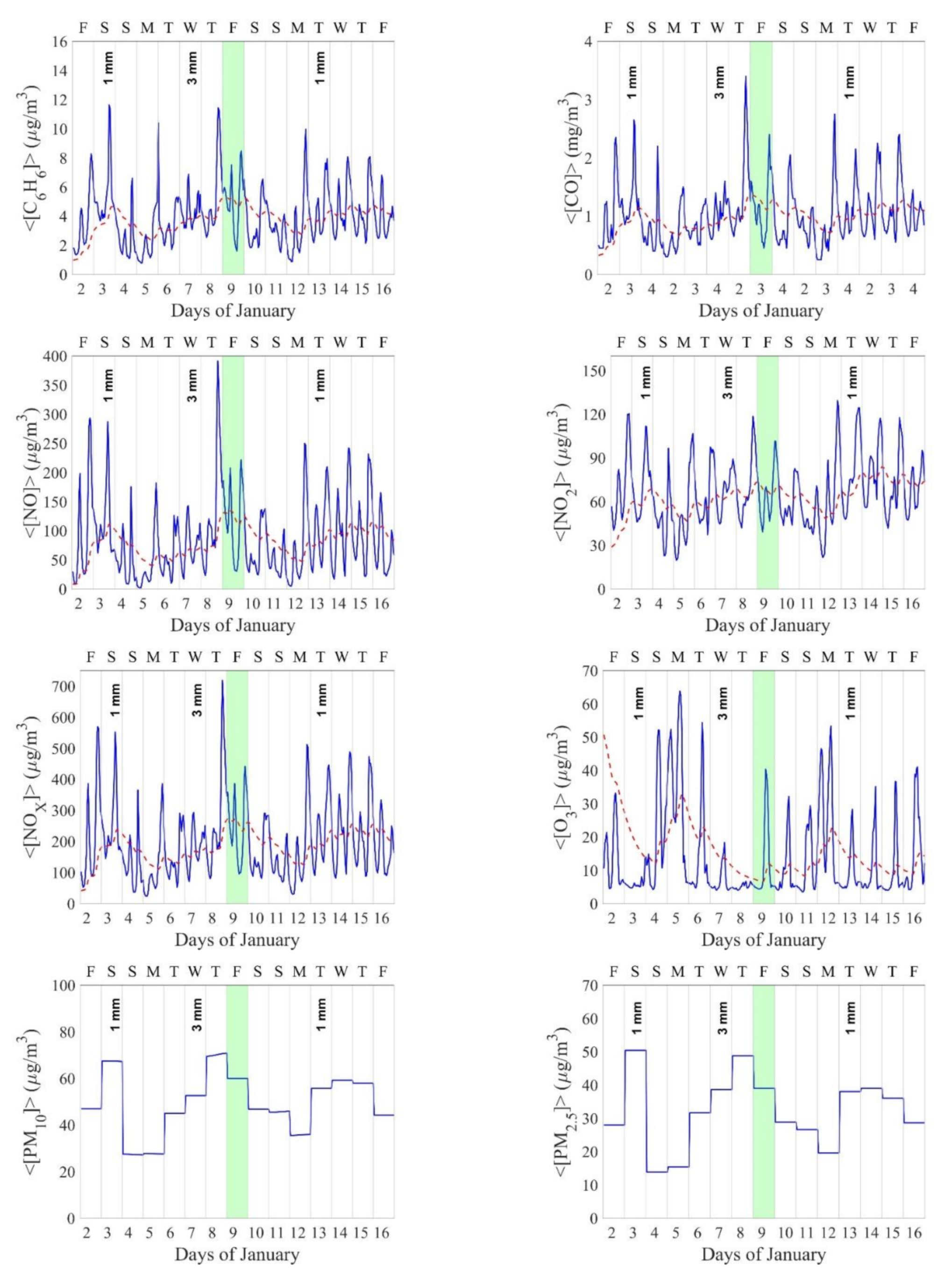
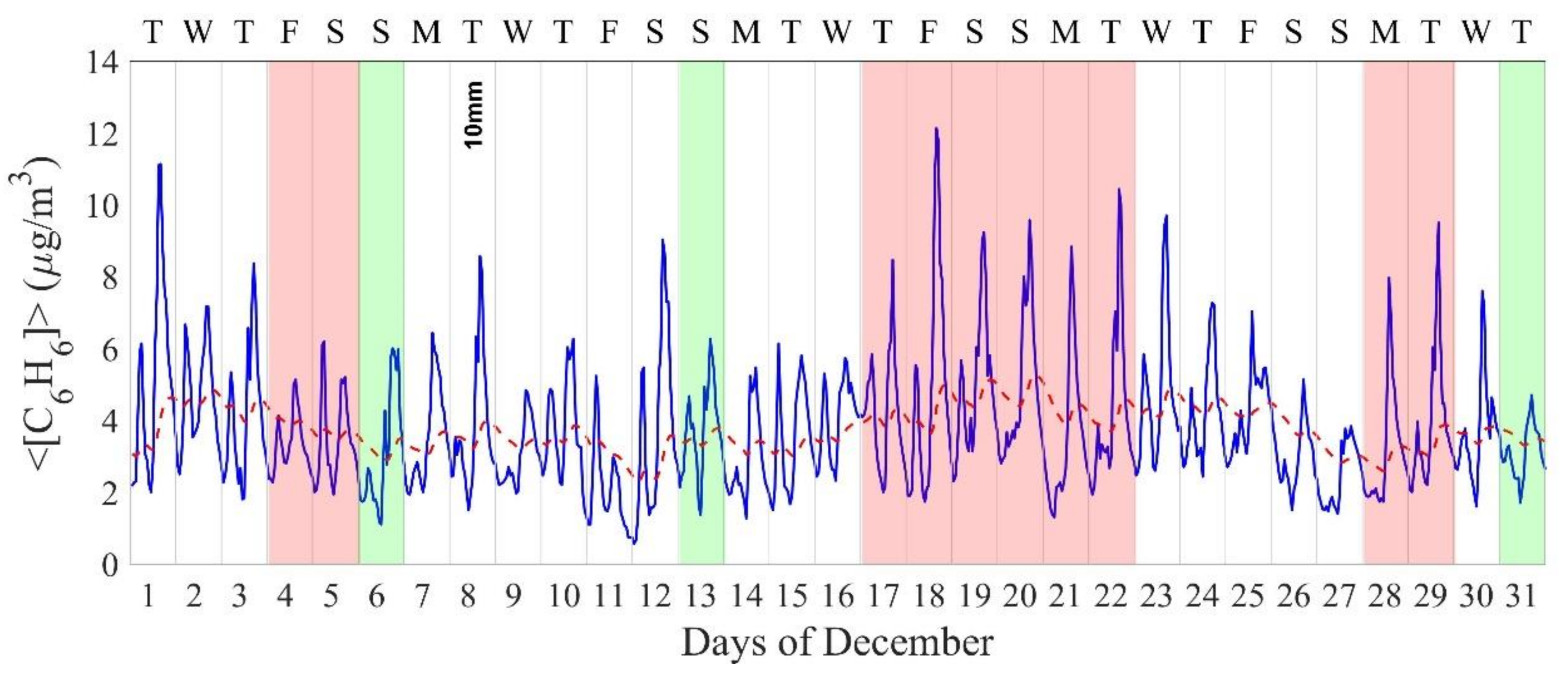
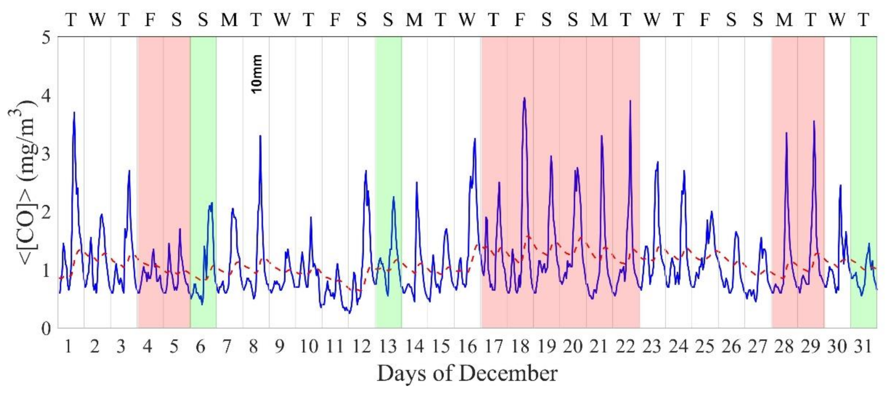
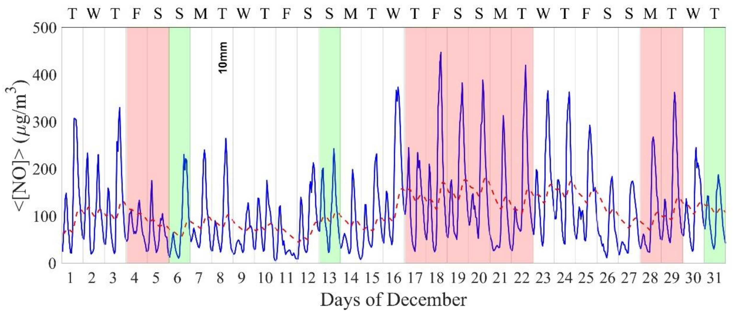
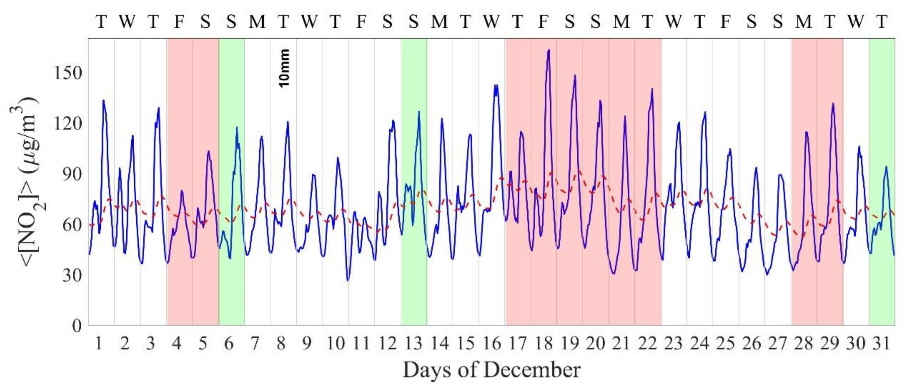
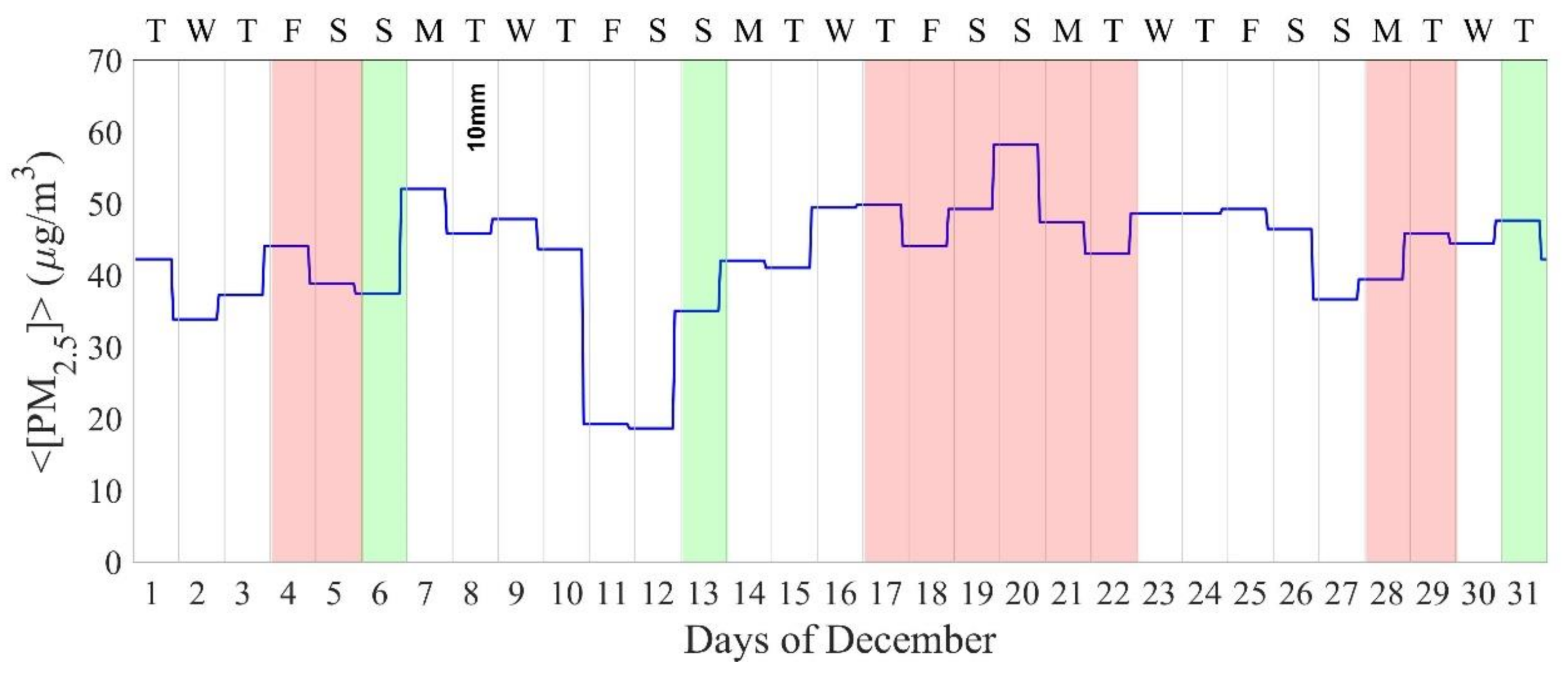
3.4. Pollution Concentrations Counter Measurements Efficacy Analysis

The main measures adopted in Italy to reduce pollutant concentrations are aimed at reducing the urban traffic with two types of strategy: rotation of cars on the streets based on the number of the plate and days of a total block of urban traffic. In fact, no policy strategy is made to reduce the utilization of heating systems. In order to verify the validity of the block of urban traffic, it was taken the data of pollutant concentration in 2015 when these measures were made. In particular, in 2015 they are:

• 9 January 2015—Total block
• 1 February 2015—Total block
• 15 November 2015—Total block
• 4/5 December 2015—Alternate plates
• 6 December 2015—Total block
• 13 December 2015—Total block
• 17/18 December 2015—Alternate plates
• 19/20 December 2015—Alternate plates
• 21/22 December 2015—Alternate plates
• 28/29 December 2015—Alternate plates
• 31 December 2015—Total block

Starting from the list above, it is useful to notice that the days in which the policy strategy was made are during the part of the year with the maximum pollutant levels. Chapter 3.3 has shown the fluctuation of the pollutant concentrations with the results of a high value during winter and especially from November to February.

Usually, days with a total block of cars on the streets aren’t applied after a day of rain. In Figure 5, Figure 6, Figure 7, Figure 8, Figure 9, Figure 10, Figure 11, Figure 12, Figure 13, Figure 14 and Figure 15 the red band identifies the days of alternated plates, the green band identifies the total block of traffic, the blue line is the hourly pollutant concentration and the red dashed line is the daily mean pollutant concentration. In the charts are also shown the days with precipitation, expressed in mm.

In the days of the block of the urban traffic, both for the alternate plate or total block cases, the levels of pollutant concentrations are quite the same. As shown from the dashed red line representing the daily mean pollutant concentration, the level isn’t affected by the policy strategy whenever it is an alternate plate or total block case. Focusing on the total block plate it is possible to notice a decrease of the particular matters [PM₁₀] and [PM_2.5] during November, January, and February in the following days. Nevertheless, this effect doesn’t appear in December and it is possible to affirm that this kind of policy strategy can’t have positive effects regarding the reduction of the pollutant emissions from urban traffic. About the alternate plates strategy, there aren’t effects in the day and in the following days of application suggesting that also this kind of strategy didn’t give any positive effect.

Figure 5, Figure 6, Figure 7, Figure 8, Figure 9, Figure 10, Figure 11, Figure 12, Figure 13, Figure 14 and Figure 15 reported the magnitude of rain in the period near the policy strategy thanked to reduce pollutant emissions. These values are useful in order to verify if the variation of the pollutant concentration can depend on the quantity of rain. Regarding the period taken into account seems that neither the rain can have a positive effect in order to reduce the pollutant concentrations.

The analysis of actual counter measurements adopted in Italy leads to affirming that in Rome, and in more general in Italian cities, the policy strategy doesn’t make a sensible variation of the pollutant concentrations. Every time there is the adoption of an alternate plate or total block of urban traffic there isn’t a variation of the pollutant levels during the day of application of the measure and in the following days.

4. Conclusions

Compliance with air quality legislation is a great challenge for modern society, in which industries, urban traffic, and building heating systems are the sources of a large number of pollutants that lead the values of concentrations beyond the allowed limits. In Italy often the policy and environmental strategies aimed to reduce the pollutant concentrations were taken in the same way for the whole country despite that there is an extreme variability of the geography, climatic, population density, industrial structures conditions. In this study, a correlation of pollutant concentration between the different sites of the Lazio region and at the same time inside the Rome city, which is very vast and has different types of build-up, greening, and traffic conditions, was investigated. Finding a pollutant level correlation can help the environmental management of each area.

This study traces its basis on pollutant data taken from stations of ARPA LAZIO Italian organization and from the analysis done by Battista et al. in 2016 [2] and 2017 [54]. This work aims to analyze the pollutant condition in Rome and in the other provinces of the Lazio region with qualitative and quantitative analysis.

Starting from this analysis, it is possible to affirm that the pollutant concentrations trend for the Rome Green Band area is the same of the suburbs of Rome and of all the provinces of Lazio. It was found that the average cross-correlation values range from 0.18 for [SO₂] to 0.88 for [PM₁₀]. Despite the value of [SO₂] the average cross-correlation is always higher than 0.4 indicating that the pollutant concentration of Roma Green Band area with the suburbs or province ones have the same trend. Analyzing the cross-correlation values for rural areas, that are usually placed with low presence of buildings and consequently the low presence of heating systems and a low number of vehicles circulating in the area, it was found that the proximity to Rome city influences the levels of pollution whenever the location is a rural or urban area, else have low or high traffic levels. Apart from the Ozone, the higher pollutant concentrations are in the winter and especially in December due to the increase of urban traffic for Christmas and the use of building heating systems. On the other hand, rural areas that are far from cities don’t have the same pollutant concentration behavior especially due to the low presence of traffic.

The update of the laws in pollutant emissions leads to the decrease year after year of pollutant concentrations, excluding the ozone that has an opposite trend. Excluding the [O₃], which have an opposite trend despite the other pollutant concentrations, the average difference of pollutant level year after year is about −1.6% for winter and −4.1% for spring-autumn with a range from 1.3% to −3.2% in winter and from −1.4% to −6.2% in spring-autumn. The presence of heating systems brings to a significant increase of the pollutant concentrations during the year with a difference from winter to spring-autumn of about 58.8% with a range from 20.1% to 127.4% excluding the [O₃].

The analysis done in spatial and temporal dependence highlights the importance to take some policy strategies to decrease the pollutant emissions both from heating systems than urban traffic because the contribution from the two anthropogenic sources is the same. Moreover, it was shown that there is a relevant variation on the pollutant level during festivity highlighting the importance to adopt a policy strategy that can help to control the emissions, especially during these periods. Focusing the attention to a typical day of the year, calculated as the average daily pollutant variation in winter and in spring-autumn, it was possible to find that there is a quite balance of levels due to urban traffic and heating systems. Higher emissions from urban traffic are referred to [NO₂], [NO_X], [CO] and [PM₁₀] with the average value for all the cities from 50.8% to 66.8%, while for building heating systems are [C₆H₆], [NO] and [PM_2.5] with the average value for all the cities from 55.2% to 65.6%. In Rome city, the percentage is higher for urban traffic for the most pollutant concentration despite the other provinces. However, considering the average values for all the cities and for all the pollutant concentrations it is possible to notice that 50% of emissions are from urban traffic and 50% are for building heating systems. From this aspect, the policy strategy needs to have attention to both the pollutant sources paying more attention in the time of the time in which there are the most traffic or the more plants turned on, that is in the morning at about 9 a.m. and in the evening at about 7 p.m.

In Italy, the adopted counter measurement to pollutant emissions is focused on the adoption of alternate plate or total block of urban traffic, and no policy strategy is done to reduce the utilization of the heating systems. To verify the validity of this kind of technique, it was taken the data of occurrence of this Italian policy strategy in Rome in 2015. The analysis highlight that the use of an alternate plate or total block of urban traffic does not give any reduction of the pollutant concentrations. So, it can be affirmed that in Rome, and in more general Italian cities, the policy strategy doesn’t lead to a sensible variation of the pollutant concentrations. Every time there is the adoption of an alternate plate or total block of urban traffic there isn’t a variation of the pollutant levels during the day of application of the measure and in the following days. It is worth noticing that during the 2015 year there was only 11 policy intervention on the urban traffic, and it seems that spots counter measurements can’t have a positive effect to reduce the pollutant concentrations.

Future steps of this research are aimed at creating a numerical model of the city of Rome able to investigate the possible policy strategies that can be used in the city and in more general in Italian urban areas. For example, it will be interesting to analyze the adoption of high-efficiency thermal plants in order to reduce the heating systems emissions, as the introduction of limitation to the vehicle circulation by adopting counter measurement like an alternate plate or total block of urban traffic in continuous during the time. Furthermore, the analysis was conducted with data from 2006 to 2015 in which there were no services like car-sharing or the electric scooter in the Italian cities that, in recent years, have a great diffusion. In this point of view, a future study can be done to analyze the impact of this technology in the reduction of urban traffic emissions.

References

1. IARC. IARC Monographs on the Evaluation of Carcinogenic Risks to Humans, Human Papillomaviruses; IARC: Lyon, France, 2007; Volume 90. [Google Scholar]
2. Battista, G.; Pagliaroli, T.; Mauri, L.; Basilicata, C.; Vollaro, R.D.L. Assessment of the Air Pollution Level in the City of Rome (Italy). Sustainability 2016, 8, 838. [Google Scholar] [CrossRef] [Green Version]
3. Schiavon, M.; Redivo, M.; Antonacci, G.; Rada, E.C.; Ragazzi, M.; Zardi, D.; Giovannini, L. Assessing the air quality impact of nitrogen oxides and benzene from road traffic and domestic heating and the associated cancer risk in an urban area of Verona (Italy). Atmos. Environ. 2015, 120, 234–243. [Google Scholar] [CrossRef]
4. Lim, S.S.; Vos, T.; Flaxman, A.D.; Danaei, G.; Shibuya, K.; Adair-Rohani, H.; AlMazroa, M.A.; Amann, M.; Anderson, H.R.; Andrews, K.G.; et al. A comparative risk assessment of burden of disease and injury attributable to 67 risk factors and risk factor clusters in 21 regions, 1990–2010: A systematic analysis for the Global Burden of Disease Study 2010. Lancet 2012, 380, 2224–2260. [Google Scholar] [CrossRef] [Green Version]
5. Cohen, A.J.; Samet, J.M.; Straif, K.; International Agency for Research on Cancer. Air Pollution and Cancer-IARC Scientific Publication; International Agency for Research on Cancer: Lion, France, 2013; No. 161; ISBN 9789283221616. [Google Scholar]
6. Ghedini, N.; Gobbi, G.; Sabbioni, C.; Zappia, G. Determination of elemental and organic carbon on damaged stone monuments. Atmos. Environ. 2000, 34, 4383–4391. [Google Scholar] [CrossRef]
7. Katsouyanni, K.; Touloumi, G.; Samoli, E.; Gryparis, A.; Le Tertre, A.; Monopolis, Y.; Rossi, G.; Zmirou, D.; Ballester, F.; Boumghar, A.; et al. Confounding and Effect Modification in the Short-Term Effects of Ambient Particles on Total Mortality: Results from 29 European Cities within the APHEA2 Project. Epidemiology 2001, 12, 521–531. [Google Scholar] [CrossRef] [PubMed] [Green Version]
8. Peters, A.; Wichmann, H.E.; Tuch, T.; Heinrich, J.; Heyder, J. Respiratory effects are associated with the number of ultrafine particles. Am. J. Respir. Crit. Care Med. 1997, 155, 1376–1383. [Google Scholar] [CrossRef] [PubMed]
9. Dockery, D.W.; Pope, C.A. Acute Respiratory Effects of Particulate Air Pollution. Annu. Rev. Public Health 1994, 15, 107–132. [Google Scholar] [CrossRef] [PubMed]
10. Battista, G.; Vollaro, E.D.L.; Vollaro, R.D.L. How Cool Pavements and Green Roof Affect Building Energy Performances. Heat Transf. Eng. 2021, 1–15. [Google Scholar] [CrossRef]
11. Memon, R.A.; Leung, D.Y.; Liu, C.-H. An investigation of urban heat island intensity (UHII) as an indicator of urban heating. Atmos. Res. 2009, 94, 491–500. [Google Scholar] [CrossRef]
12. Mauri, L.; Battista, G.; de Lieto Vollaro, E.D.L.; de Lieto Vollaro, R.D.L. Retroreflective materials for building’s façades: Experimental characterization and numerical simulations. Sol. Energy 2018, 171, 150–156. [Google Scholar] [CrossRef]
13. Mei, S.-J.; Hu, J.-T.; Liu, D.; Zhao, F.-Y.; Li, Y.; Wang, H.-Q. Airborne pollutant dilution inside the deep street canyons subjecting to thermal buoyancy driven flows: Effects of representative urban skylines. Build. Environ. 2019, 149, 592–606. [Google Scholar] [CrossRef]
14. Gallagher, J.; Lago, C. How parked cars affect pollutant dispersion at street level in an urban street canyon? A CFD modelling exercise assessing geometrical detailing and pollutant decay rates. Sci. Total Environ. 2019, 651, 2410–2418. [Google Scholar] [CrossRef] [PubMed]
15. Kubilay, A.; Neophytou, M.K.A.; Matsentides, S.; Loizou, M.; Carmeliet, J. The pollutant removal capacity of urban street canyons as quantified by the pollutant exchange velocity. Urban Clim. 2017, 21, 136–153. [Google Scholar] [CrossRef]
16. Oke, T.R. Street design and urban canopy layer climate. Energy Build. 1988, 11, 103–113. [Google Scholar] [CrossRef]
17. Russo, A.; Chan, W.T.; Cirella, G.T. Estimating Air Pollution Removal and Monetary Value for Urban Green Infrastructure Strategies Using Web-Based Applications. Land 2021, 10, 788. [Google Scholar] [CrossRef]
18. Britter, R.E.; Hanna, S.R. Flow anddispersion inurbanareas. Annu. Rev. Fluid Mech. 2003, 35, 469–496. [Google Scholar] [CrossRef]
19. Sarangi, A.; Cox, C.A.; Madramootoo, C.A. Geostatistical methods for prediction of spatial variability of rainfall in a mountainous region. Trans. ASAE 2005, 48, 943–954. [Google Scholar] [CrossRef] [Green Version]
20. De la Fuente, D.; Vega, J.M.; Viejo, F.; Díaz, I.; Morcillo, M. Mapping air pollution effects on atmospheric degradation of cultural heritage. J. Cult. Herit. 2013, 14, 138–145. [Google Scholar] [CrossRef] [Green Version]
21. Morgan, G.; Corbett, S.; Wlodarczyk, J.; Lewis, P. Air pollution and daily mortality in Sydney, Australia, 1989 through 1993. Am. J. Public Health 1998, 88, 759–764. [Google Scholar] [CrossRef] [Green Version]
22. Rakowska, A.; Wong, K.C.; Townsend, T.; Chan, K.L.; Westerdahl, D.; Ng, S.; Mocnik, G.; Drinovec, L.; Ning, Z. Impact of traffic volume and composition on the air quality and pedestrian exposure in urban street canyon. Atmos. Environ. 2014, 98, 260–270. [Google Scholar] [CrossRef]
23. Whitworth, K.W.; Symanski, E.; Lai, D.; Coker, A.L. Kriged and modeled ambient air levels of benzene in an urban environment: An exposure assessment study. Environ. Health 2011, 10, 1–10. [Google Scholar] [CrossRef] [Green Version]
24. Ella, V.B.; Melvin, S.W.; Kanwar, R.S. Spati al analysis of no3-n concentration in glacial till. Trans. ASAE 2001, 44, 317. [Google Scholar] [CrossRef]
25. Gupta, P.; Sarma, K. Spatial distribution of various parameters in groundwater of Delhi, India. Cogent Eng. 2016, 3. [Google Scholar] [CrossRef]
26. Shulgan, R.; Kibukevich, O.; Yanchuk, O.; Nikolaichuk, K. Grid-model of natural agricultural zoning. Geodesy Cartogr. 2017, 43, 22–27. [Google Scholar] [CrossRef] [Green Version]
27. Demetriou, D. The assessment of land valuation in land consolidation schemes: The need for a new land valuation framework. Land Use Policy 2016, 54, 487–498. [Google Scholar] [CrossRef]
28. Kwiecień, J.; Szopińska, K. Mapping Carbon Monoxide Pollution of Residential Areas in a Polish City. Remote Sens. 2020, 12, 2885. [Google Scholar] [CrossRef]
29. Maleki, H.; Sorooshian, A.; Goudarzi, G.; Baboli, Z.; Birgani, Y.T.; Rahmati, M. Air pollution prediction by using an artificial neural network model. Clean Technol. Environ. Policy 2019, 21, 1341–1352. [Google Scholar] [CrossRef]
30. Shih, D.-H.; To, T.; Nguyen, L.; Wu, T.-W.; You, W.-T. Design of a Spark Big Data Framework for PM2.5 Air Pollution Forecasting. Int. J. Environ. Res. Public Health 2021, 18, 7087. [Google Scholar] [CrossRef] [PubMed]
31. Huang, C.-J.; Kuo, P.-H. A Deep CNN-LSTM Model for Particulate Matter (PM2.5) Forecasting in Smart Cities. Sensors 2018, 18, 2220. [Google Scholar] [CrossRef] [Green Version]
32. Fan, J.; Li, Q.; Hou, J.; Feng, X.; Karimian, H.; Lin, S. A Spatiotemporal Prediction Framework for Air Pollution Based on Deep RNN. ISPRS Ann. Photogramm. Remote Sens. Spat. Inf. Sci. 2017, IV-4/W2, 15–22. [Google Scholar] [CrossRef] [Green Version]
33. Prihatno, A.; Nurcahyanto, H.; Ahmed, F.; Rahman, H.; Alam, M.; Jang, Y. Forecasting PM2.5 Concentration Using a Single-Dense Layer BiLSTM Method. Electronics 2021, 10, 1808. [Google Scholar] [CrossRef]
34. Pappa, A.; Kioutsioukis, I. Forecasting Particulate Pollution in an Urban Area: From Copernicus to Sub-Km Scale. Atmosphere 2021, 12, 881. [Google Scholar] [CrossRef]
35. Iglesias-Gonzalez, S.; Huertas-Bolanos, M.; Hernandez-Paniagua, I.; Mendoza, A. Explicit Modeling of Meteorological Explanatory Variables in Short-Term Forecasting of Maximum Ozone Concentrations via a Multiple Regression Time Series Framework. Atmosphere 2020, 11, 1304. [Google Scholar] [CrossRef]
36. Cho, S.; Park, H.; Son, J.; Chang, L. Development of the Global to Mesoscale Air Quality Forecast and Analysis System (GMAF) and Its Application to PM2.5 Forecast in Korea. Atmosphere 2021, 12, 411. [Google Scholar] [CrossRef]
37. Cordano, M.; Frieze, I.H. Pollution Reduction Preferences of U.S. Environmental Managers: Applying Ajzen’s Theory of Planned Behavior. Acad. Manag. J. 2000, 43, 627–641. [Google Scholar] [CrossRef]
38. Tian, J.; Chen, D. A semi-empirical model for predicting hourly ground-level fine particulate matter (PM2.5) concentration in southern Ontario from satellite remote sensing and ground-based meteorological measurements. Remote Sens. Environ. 2010, 114, 221–229. [Google Scholar] [CrossRef]
39. Russell, A.G.; McCue, K.F.; Cass, G.R. Mathematical modeling of the formation of nitrogen-containing air pollutants. 1. Evaluation of an Eulerian photochemical model. Environ. Sci. Technol. 1988, 22, 263–271. [Google Scholar] [CrossRef]
40. Suleiman, A.; Tight, M.; Quinn, A. Applying machine learning methods in managing urban concentrations of traffic-related particulate matter (PM10 and PM2.5). Atmos. Pollut. Res. 2019, 10, 134–144. [Google Scholar] [CrossRef]
41. Zheng, W.; Li, X.; Yin, L.; Wang, Y. Spatiotemporal heterogeneity of urban air pollution in China based on spatial analysis. Rend. Lincei 2016, 27, 351–356. [Google Scholar] [CrossRef]
42. Zhang, J.; Mauzerall, D.; Zhu, T.; Liang, S.; Ezzati, M.; Remais, J.V. Environmental health in China: Progress towards clean air and safe water. Lancet 2010, 375, 1110–1119. [Google Scholar] [CrossRef] [Green Version]
43. Roma. Capitale Piano Generale del Traffico Urbano di Roma Capitale. Available online: https://romamobilita.it/sites/default/files/pdf/pubblicazioni/PGTU_aprile_2015.pdf (accessed on 2 October 2016).
44. ARPA. Lazio Centro Regionale della Qualità dell’Aria. Available online: http://www.arpalazio.net/ (accessed on 2 October 2016).
45. Repubblica Italiana. DPR 203/88-Attuazione Delle Direttive CEE Numeri 80/779. 82/884. 84/360 e 85/203 Concernenti Norme in Materia di Qualità Dell’aria Relativamente a Specifici Agenti Inquinanti. e di Inquinamento Prodotto Dagli Impianti Industriali. ai Sensi Dell’art; Repubblica Italiana DPR: Rome, Italy, 1988. [Google Scholar]
46. European Commission. Directive 2008/50/EC of the European Parliament and of the Council of on Ambient Air Quality and Cleaner Air for Europe. Off. J. Eur. Union 2008, 152, 1–144. [Google Scholar]
47. Repubblica Italiana. D.Lgs. 155/2010-Attuazione Della Direttiva 2008/50/CE Relativa Alla Qualità Dell’aria Ambiente e per Un’aria più Pulita in Europa; Repubblica Italiana: Rome, Italy, 2010. [Google Scholar]
48. European Commission. Available online: https://ec.europa.eu/ (accessed on 10 August 2021).
49. Lega, P.; Benedusi, L. Sistema Informativo Provinciale Delle Emissioni Inquinanti in Atmosfera; Provincia di Piacenza: Piacenza, Italy, 2000. [Google Scholar]
50. Ministero dell’Ambiente e Della Tutela del Territorio e del Mare. Relazione Sullo Stato Dell’ambiente; MATTM: Rome, Italy, 2016.
51. ISTAT. Veicoli-Pubblico Registro Automobilistico. Available online: http://dati.istat.it/Index.aspx?DataSetCode=DCIS_VEICOLIPRA# (accessed on 10 August 2021).
52. Repubblica Italiana. DPR 412/93—Regolamento Recante Norme per la Progettazione, L’installazione, L’esercizio e la Manutenzione Degli Impianti Termici Degli Edifici ai Fini del Contenimento dei Consumi di Energia, in Attuazione dell’art. 4, Comma 4, Della Legge 9 Gennaio 1991; Repubblica Italiana: Rome, Italy, 1993. [Google Scholar]
53. Kaloustian, N.; Aouad, D.; Battista, G.; Zinzi, M. Leftover Spaces for the Mitigation of Urban Overheating in Municipal Beirut. Climate 2018, 6, 68. [Google Scholar] [CrossRef] [Green Version]
54. Battista, G.; de Lieto Vollaro, R.D.L. Correlation between air pollution and weather data in urban areas: Assessment of the city of Rome (Italy) as spatially and temporally independent regarding pollutants. Atmos. Environ. 2017, 165, 240–247. [Google Scholar] [CrossRef]
Figure 1. Monitoring stations network of ARPA LAZIO used in the present study.
Applsci 11 07936 g001
Figure 2. Average pollutant concentrations trend of Rome over the decade 2006–2015 of winter (blue line) and spring-autumn (red line). Dashed lines are referred to as trend lines.
Applsci 11 07936 g002
Figure 3. Normalized pollutant concentrations of Rome in 2015. Values are referred to the subtraction of the pollutant concentration in time by time with the mean values in spring, summer, and autumn in order to decurtate the pollutant level from the urban traffic sources.
Applsci 11 07936 g003
Figure 4. Day variation of pollutant during 2015 considering the mean value hour per hour and divided from winter (blue line) to spring-autumn (red line).
Applsci 11 07936 g004aApplsci 11 07936 g004b
Figure 5. Pollutant concentration variation related to the total block of urban traffic of 9th January 2015 (green band). The blue line is the hourly pollutant concentration. The Red dashed line is the daily mean pollutant concentration. Data of daily precipitation are indicated in mm.
Applsci 11 07936 g005
Figure 6. Pollutant concentration variation related to the total block of urban traffic of 1st February 2015 (green band). The blue line is the hourly pollutant concentration. The Red dashed line is the daily mean pollutant concentration. Data of daily precipitation are indicated.
Applsci 11 07936 g006
Figure 7. Pollutant concentration variation related to the total block of urban traffic of 15th November 2015 (green band). The blue line is the hourly pollutant concentration. The Red dashed line is the daily mean pollutant concentration. Data of daily precipitation are indicated in mm.
Applsci 11 07936 g007
Figure 8. Benzene concentration variation related to the total block of urban traffic (green band) and alternated plates (red band) of December 2015. The blue line is the hourly pollutant concentration. The red dashed line is the daily mean pollutant concentration. Data of daily precipitation are indicated in mm.
Applsci 11 07936 g008
Figure 9. Carbon monoxide concentration variation related to the total block of urban traffic (green band) and alternated plates (red band) of December 2015. The blue line is the hourly pollutant concentration. The red dashed line is the daily mean pollutant concentration. Data of daily precipitation are indicated in mm.
Applsci 11 07936 g009
Figure 10. Nitric oxide concentration variation related to the total block of urban traffic (green band) and alternated plates (red band) of December 2015. The blue line is the hourly pollutant concentration. The red dashed line is the daily mean pollutant concentration. Data of daily precipitation are indicated in mm.
Applsci 11 07936 g010
Figure 11. Nitrogen dioxide concentration variation related to the total block of urban traffic (green band) and alternated plates (red band) of December 2015. The blue line is the hourly pollutant concentration. The red dashed line is the daily mean pollutant concentration. Data of daily precipitation are indicated in mm.
Applsci 11 07936 g011
Figure 12. Nitrogen oxides concentration variation related to the total block of urban traffic (green band) and alternated plates (red band) of December 2015. The blue line is the hourly pollutant concentration. The red dashed line is the daily mean pollutant concentration. Data of daily precipitation are indicated in mm.
Applsci 11 07936 g012
Figure 13. Oxone concentration variation related to the total block of urban traffic (green band) and alternated plates (red band) of December 2015. The blue line is the hourly pollutant concentration. The red dashed line is the daily mean pollutant concentration. Data of daily precipitation are indicated in mm.
Applsci 11 07936 g013
Figure 14. Particulate matter PM10 concentration variation related to the total block of urban traffic (green band) and alternated plates (red band) of December 2015. The blue line is the hourly pollutant concentration. Data of daily precipitation are indicated in mm.
Applsci 11 07936 g014
Figure 15. Particulate matter PM2.5 concentration variation related to the total block of urban traffic (green band) and alternated plates (red band) of December 2015. The blue line is the hourly pollutant concentration. Data of daily precipitation are indicated in mm.
Applsci 11 07936 g015