Data-Driven Control Algorithm for Snake Manipulator

Abstract

In some environments where manual work cannot be carried out, snake manipulators are instead used to improve the level of automatic work and ensure personal safety. However, the structure of the snake manipulator is diverse, which renders it difficult to establish an environmental model of the control system. It is difficult to obtain an ideal control effect by using the traditional manipulator control method. In view of this, this paper proposes a data-driven snake manipulator control algorithm. After collecting data, the algorithm uses the strong learning and decision-making ability of the deep deterministic strategy gradient to learn these system data. A data-driven controller based on the deep deterministic policy gradient was trained in order to solve the manipulator system control problem when the control system environment model is uncertain or even unknown. The data of simulation experiments show that the control algorithm has good stability and accuracy in the case of model uncertainty.

1. Introduction

Existing manipulator control theory can be divided into three categories: (1) Accurate mathematical models are required, such as optimal control strategies, linear or nonlinear control strategies, and pole assignment methods. Some (2) mathematical models are known, such as sliding mode variable structure control, fuzzy control, adaptive control, and intelligent control. (3) The mathematical model is unknown, or it is difficult to establish a mathematical model, such as iterative learning control, model-free adaptive control, and other data-driven control strategies [1]. Currently, the commonly adopted control strategies of manipulators include PID control, fuzzy control, adaptive control, and hybrid control strategy. Mendes designed an adaptive fuzzy controller to solve the contact problem of a manipulator [2]. However, with continuous improvement of the control requirements of manipulators, the scale of control systems is increasing, there are a large number of coupling phenomena between the systems, and the traditional manipulator control strategy has been unable to meet the control requirements. Due to their strong self-learning ability and nonlinear system mapping ability, neural networks have been introduced into manipulator control to compensate for the uncertainty of manipulator models. Aiming at the trajectory tracking control problem caused by uncertainty and disturbance of the manipulator, Vu proposed a robust adaptive control strategy based on a fuzzy wavelet neural network system with dynamic structure. The control strategy can effectively reduce system error and can improve the control accuracy of the manipulator system [3,4]. Concerning the problem of the unknown dynamic model of a manipulator, Yu proposed an adaptive neural network tracking control strategy based on a disturbance observer, which is used to compensate for the unknown disturbance of the system [5]. Jung proposed an improved sliding mode control method based on an RBF neural network to solve the problem of nonlinear function gain selection of a sliding mode controller and the uncertainty of the three-link manipulator model [6].

The hybrid control strategy of neural networks [7] and classical strategy can improve the control performance of the manipulator and can improve its application in many fields, such as stirring, welding, polishing, and assembly. However, with continuous improvement in industrial production accuracy, the neural network model’s uncertainty compensation has been unable to meet control accuracy requirements. Therefore, the deep neural network algorithm was introduced into manipulator control. Due to its strong perception and decision-making ability, deep reinforcement learning can perceive the response of the environment to change and improve the accuracy of the behavior of the agent. Therefore, deep reinforcement learning is more widely used in deep neural network algorithms [8,9].

Deep Reinforcement Learning (DRL) is an artificial intelligence method that combines deep learning with a perceptual ability and reinforcement learning with a decision-making ability. DRL can be divided into two categories: value-based function and strategy-based gradient. The value-based learning algorithm is mainly an approximate representation of the value function. The representative algorithms are the Deep Q Network (DQN) algorithm, Nature DQN algorithm, Double DQN algorithm [10], prioritized replay DQN algorithm [11], and Dueling DQN algorithm [12]. The representative algorithm based on strategy learning is the Policy Gradient algorithm [13]. The algorithms that combines strategy and value are the Actor-Critic algorithm [14], the Deep Deterministic Policy Gradient (DDPG) algorithm, and the Asynchronous Advantage Actor-Critic (A3C) [15]. The algorithms are summarized in

Table 1. Classical Deep reinforcement learning algorithms.

Classification Algorithm	Algorithm Name	Algorithm Improvement
	Nature DQN	Two identical Q network structures.
Value-based reinforcement learning (DQN)	Double DQN	A choice of action between decoupling target Q value and the calculation of target Q value.
	Prioritized replay DQN	The sample is prioritized.
	Dueling DQN	The value function of the Q network is divided into two parts: value function and advantage function.
Strategy-based reinforcement learning method	Policy gradient	Value-based methods are replaced by policy-based methods.
	Actor-critic	The two methods, namely policy-based and value-based, are combined.
Hybrid algorithm actor-critic	Asynchronous advantage actor-critic (A3C)	Asynchronous training framework, network structure optimization, and evaluation point optimization. A general asynchronous concurrent reinforcement learning framework
	Deep deterministic policy gradient (DDPG)	Two actor networks and two critic networks, a total of four neural networks, are used to update the model parameters iteratively.

[16].

DRL has been proven to be effective in solving complex control problems of manipulators in OpenAI, such as operating [17], grasping [18,19], and mobile tasks [20,21]. Luo applied the DRL strategy to the assembly task of a manipulator. The device completed a task that could not be realized using the traditional control strategy [22]. Through the priority division of the DRL network, Wu realized high-precision millimeter-scale automatic assembly technology [23]. Wen designed an obstacle avoidance algorithm based on DDPG, which solved the convergence problem of the obstacle avoidance motion of the manipulator and ensured its continuity and stability [24].

The contribution of this paper is to propose a data-driven snake manipulator control strategy to solve the control problem of snake manipulators in some complex environments. The main work is as follows:

(1)

Based on the model control method, a control system of a two-link model snake manipulator based on DDPG was designed. First, according to the structure of the snake manipulator and the Lagrangian dynamic equation, the dynamic model of the two-link snake manipulator was established. Second, the Q network model and action network model of the DDPG agent were designed. Finally, the simulation results show that the control strategy based on DDPG has good convergence and strong anti-jamming ability.

(2)

In order to solve the problem of model uncertainty, a data-driven control method of the snake manipulator is proposed. When the number of connecting rods of the serpentine manipulator increases and the environment becomes complex, it is difficult to establish the model of an integral snake manipulator that renders the control effect of the model-based control strategy poor. In view of this, a data-driven control method based on DDPG is proposed. First, the data-driven control method requires a large number of input and output data, and the data set was established by using the results of the traditional control method as the training sample of this method. Second, the DDPG agent model was designed according to the input and output parameters. Finally, based on simulation and comparative results analysis, the feasibility and superiority of the control method was verified.

The main sections of this paper are as follows. The Section 1 mainly introduces the control methods currently applied to the manipulator. It briefly combs through the control method of the manipulator, focusing on the DRL algorithm and its application in the manipulator. Based on this, aiming at the problems in the application of the snake manipulator, the main innovation of this paper is pointed out. Combined with previous research work on DRL in manipulators, Section 2 outlines the chosen DRL algorithm and DDPG algorithm used in this study. The main structure, workflow, and related calculation methods of DDPG are described in detail. In the Section 3, the design of the DDPG control method simulation of the two-link snake manipulator is explained. The method of establishing the environment object and agent of the DDPG control system is introduced in detail. This mainly includes the two-link dynamic model of the serpentine manipulator, Q network design, and action network design. The simulation results show that the DDPG algorithm is effective and superior in the control of snake manipulators. Section 4, based on the research outlined in the Section 3, reports that it is difficult to establish the entire snake manipulator model, with significant error in the accuracy of the model, which reduces the stability and accuracy of the control system. In view of this, a data-driven control method of the snake manipulator is proposed in this paper. The simulation experiment of this method was designed, and the simulation results verify the feasibility of the method. In addition, this method not only avoids the complicated task of establishing the manipulator model but also improves the stability and accuracy of the control system.The data-driven control algorithm uses the existing motion data of the serpentine robot. All the motion data of the serpentine robot are integrated, and its motion database is established. The DDPG is used to train using the data in the database, and the current best motion path is obtained. With the increasing amount of data in the database, the accuracy and stability of robot control continue to improve. Section 5 summarizes the work of this paper.

2. Deep Deterministic Policy Gradient

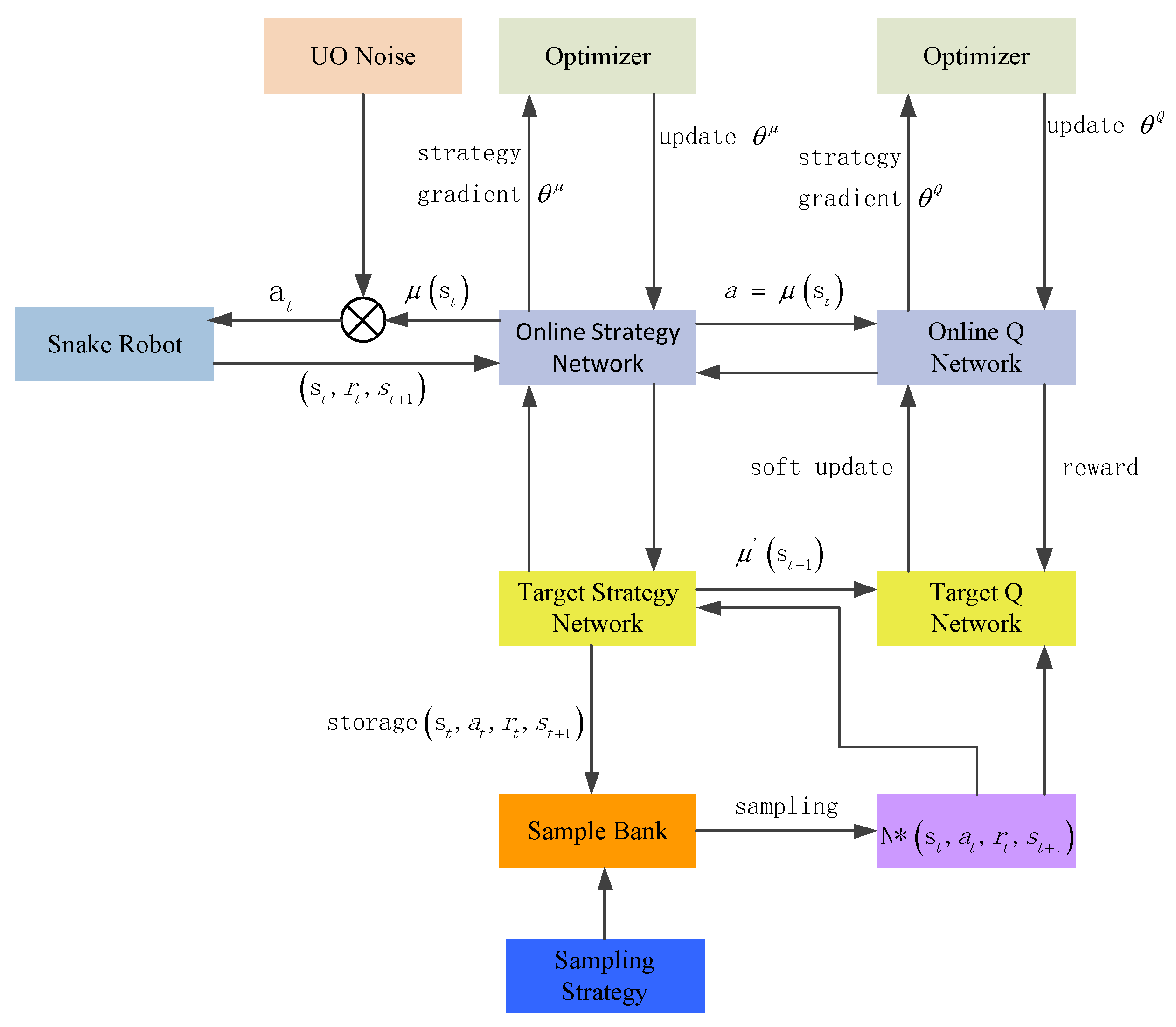
In the study of motion control of a two-link manipulator, Jianping Wang compared 3 kinds of DRL algorithms: A3C, DPPO, and DDPG. He found that the DDPG algorithm has the best convergence effect on the control system. The convergence reward value of the algorithm is the most stable [25]. Since the DDPG algorithm has a better control effect on the manipulator [26] and the motion of the snake manipulator is mainly continuous, the application of the DDPG algorithm was studied in this work. DDPG adds a deterministic strategy network on the basis of the DQN to output action values; thus, compared with the DQN, it only needs to learn the Q network, while DDPG also needs to learn the strategy network. The network structure of DDPG is shown in Figure 1.

From the figure, we can observe that DDPG has four networks: the current action network, the target action network, the current Q network, and the target Q network. The current action network is mainly used to update the policy network parameter ${\delta }^{\mu }$. The network selects the current action A through the current state S. By utilizing target action network sampling, one state $S^{\prime }$ selects the optimal next action, and its network parameter ${\delta }^{{\mu }^{\prime }}$ duplicates the parameter value of ${\delta }^{\mu }$. The current Q network is mainly used to update the value network parameter ${\theta }^Q$ and to calculate the current Q value. The target Q network is used to calculate the $Q^{\prime }$ part of the Q value, and the network parameter ${\delta }^{Q^{\prime }}$ copies the parameter ${\theta }^Q$. The two processes of updating network parameters are different. The current network uses the SGD algorithm to update network parameters. The target network uses the soft update algorithm to update the network parameters, as shown in Equation (1). By using the soft update algorithm, the change in the target network parameters is small, and the training is easy to converge, but the learning speed is slow.

$$\begin{array}{c}\hfill {\theta }^{Q^{\prime }}\leftarrow \delta {\theta }^Q+(1-\tau ){\theta }^{Q^{\prime }}\\ \hfill {\theta }^{{\mu }^{\prime }}\leftarrow \delta {\theta }^{\mu }+(1-\tau ){\theta }^{{\mu }^{\prime }}\end{array}$$

(1)

In Equation (1), ${\theta }^{Q^{\prime }}$ denotes the target Q network parameters. ${\theta }^Q$ denotes the current Q network parameters. The current network parameters ${\theta }^{\mu }$ and target network parameters ${\theta }^{{\mu }^{\prime }}$ are constructed by policy $\mu$. $\delta$ is the update coefficient, and the value is often 0.1 or 0.01.

For the definition of the network loss function, the current Q network loss function is similar to that in the DQN, mainly using mean square error, as shown in Formula (2).

$$Loss=\sum _{i=1}^m{(r_i-Q(s_i,a_i,\omega ))}^2$$

(2)

In Formula (2), Loss denotes the loss function. $r_i$ denotes the reward value of i moment. $Q(s_i,a_i,\omega )$ denotes the current Q network Q value calculation function. Since the deterministic strategy is adopted in the current action network, its loss function is different from that of PG and A3C.

$${▽}_J\left(\theta \right)=\sum _i^m[{▽}_{a}Q(s_i,a_i,\omega ){\mid }_{s=s_i,a={\pi }_{\theta }\left(s\right)}*{▽}_{\theta *{\pi }_{theta}\left(s\right)}{\mid }_{s=s_i}]$$

(3)

In Formula (3), ▽ denotes the gradient decreases. ${\pi }_{\theta }\left(s\right)$ denotes the action selection strategy. For the loss function, the greater the Q value of the target action, the smaller the Loss. The smaller the Q value, the greater the Loss; thus, the status network returns to a negative Q value.

$$J\left(\theta \right)=-\sum _i^{m}Q(s_i,a_i,\omega )$$

(4)

In Formula (4), $s_i$ denotes the state of the manipulator at i moment, including joint angle and angular velocity. $a_i$ denotes the moment value of the manipulator at time i, which is transformed from the state $s_i$ to $s_{i+1}$ through the dynamic model.

$$r_{Time}=\sum _{i=t}^{Time}{\gamma }^{i-t}*r(s_i,a_i)$$

(5)

In Formula (5), $\gamma$ denotes the weighted value of the reward, the range of the value is $\left[\begin{array}{cc}0& 1\end{array}\right]$, and $Time$ denotes the total time. $r(s_i,a_i)$ is used to calculate the single-step reward value obtained by the dynamic model after performing the behavior $a_i$ in the state $s_i$. $r_{Time}$ denotes the weighted total value of all single-step awards r from the current state to a certain state throughout the process.

3. Simulation of DDPG Control Based on 2-Link Model

In order to verify whether the DDPG algorithm can be feasibly and effectively applied to the space manipulator, a DDPG control simulation based on two connecting rods was designed, as outlined in this section. In addition, a 2-link model lays the foundation for the establishment of the whole model.

3.1. Overall Design Scheme of Control System

The DDPG-based control system is shown in Figure 2. According to the given parameters of the target trajectory point, the angular value, angular velocity value, and angular acceleration value of each joint moving to the target point are calculated by using the ridge method. These parameters are used as input to the DDPG controller. The DDPG agent is trained, saving the agent that meets the conditions, and finally the state value with the lowest reward value is the output. The position of the actual trajectory point is obtained by the forward kinematics of the manipulator. The control precision value is obtained from the error between the actual position and the target position.

3.2. Environmental Object Establishment

A modular design method was adopted for the snake manipulator in this study to facilitate equipment maintenance. In order to improve the flexibility of the manipulator, a 1-joint 2-degrees-of-freedom structure was adopted to enable the manipulator to move in both the yaw and pitch directions, and the three-dimensional motion of the manipulator was realized. A structure diagram of the snake manipulator model is shown in Figure 3. Due to the large number of structural joints, a 2-joint structure was used as an example in this study to establish the dynamic model.

(1) Definition of input signal: In this experiment, the joint torque of the 2-link manipulator was used as the input signal of the environment object.

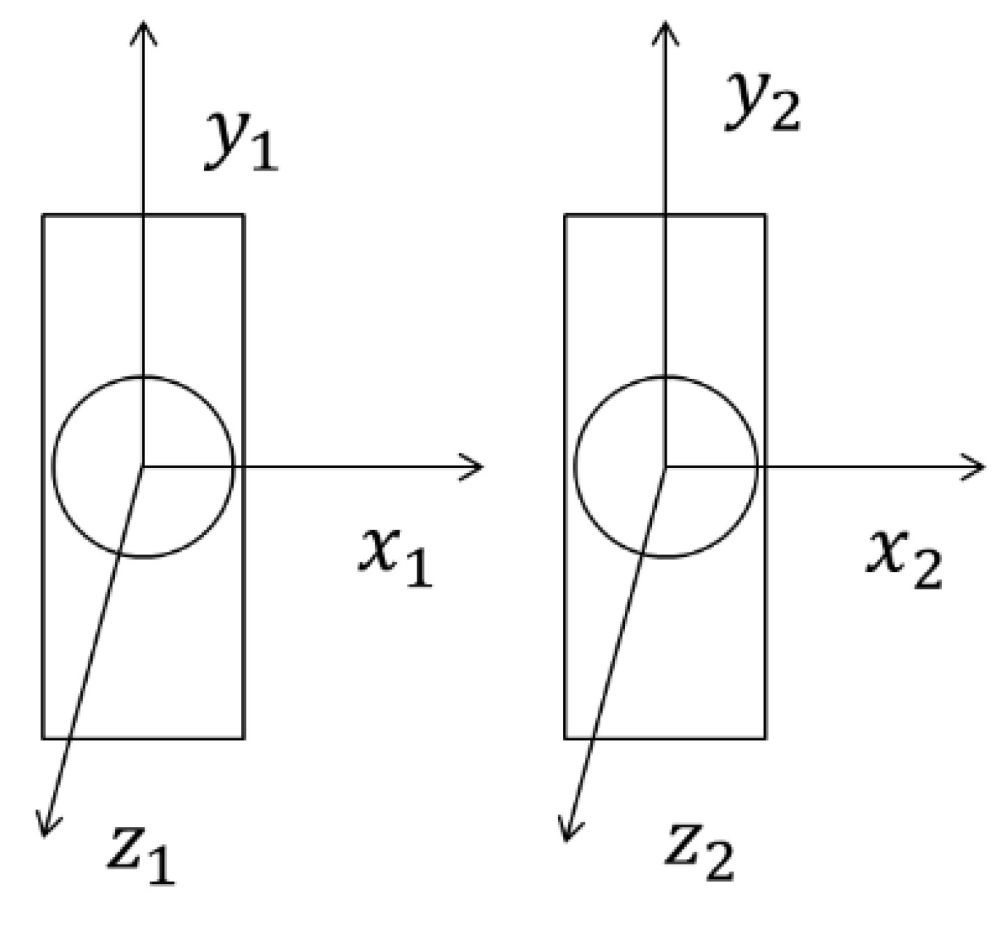
(2) Establishing a dynamic equation to evaluate the environment: The dynamic model of the two connecting rods was established according to the Lagrangian dynamic method. The joint coordinate system of the manipulator is shown in Figure 4. The yaw angle is $\alpha$. The pitch angle is $\beta$.

Suppose that the mass of the connecting rod is concentrated at the center of mass; the inertia tensor of the connecting rod is set to 0. Therefore, according to the Lagrange formula, the kinetic energy and potential energy of each connecting rod are expressed as follows.

$$E_{k1}=\frac{1}{2}{m}_1\dot{P_{c1}^T}\dot{P_{c1}}$$

(6)

$$E_{p1}=m_{1}g{L}_{c1}sin\left({\beta }_1\right)$$

(7)

$$E_{k2}=\frac{1}{2}{m}_2\dot{P_{c2}^T}\dot{P_{c2}}$$

(8)

$$E_{p2}=m_{2}g(asin\left({\beta }_1\right)+L_{c2}sin({\beta }_1+{\beta }_1))$$

(9)

In Formulas (6)–(9), $E_{k1}$ denotes the kinetic energy of the first connecting rod; $E_{p1}$ denotes the potential energy of the first connecting rod; $\dot{P_{c1}}$ denotes the velocity at the center of mass of the first connecting rod; “g” denotes gravitational acceleration; “a” represents the length of the connecting rod; and $L_{c1}$ denotes the length of the center of mass of the first connecting rod, etc. The definitions are consistent for all formulas in this paper.

$$P_{c1}=\left[\begin{array}{c}{L}_{c1}cos\left({\alpha }_1\right)cos\left({\beta }_1\right)\\ L_{c1}sin\left({\beta }_1\right)\\ -L_{c1}sin\left({\alpha }_1\right)cos\left({\beta }_1\right)\end{array}\right]$$

(10)

$$P_{c1}=\left[\begin{array}{c}a*cos\left({\alpha }_1\right)cos\left({\beta }_1\right)+L_{c2}cos({\alpha }_1+{\alpha }_2)cos({\beta }_1+{\beta }_2)\\ a*sin\left({\beta }_1\right)+L_{c2}sin({\beta }_1+{\beta }_2)\\ -a*sin\left({\alpha }_1\right)cos\left({\beta }_1\right)-L_{c2}sin({\alpha }_1+{\alpha }_2)cos({\beta }_1+{\beta }_2)\end{array}\right]$$

(11)

${\theta }_1={\left[\begin{array}{ccc}0& {\alpha }_1& {\beta }_1\end{array}\right]}^{\mathrm{T}}$ denotes the rotation angle of joint 1. $\dot{{\theta }_1}={\left[\begin{array}{ccc}0& \dot{{\alpha }_1}& \dot{{\beta }_1}\end{array}\right]}^{\mathrm{T}}$ denotes the angular velocity of joint 1. $\ddot{{\theta }_1}={\left[\begin{array}{ccc}0& \ddot{{\alpha }_1}& \ddot{{\beta }_1}\end{array}\right]}^{\mathrm{T}}$ denotes the angular acceleration of joint 1. The angular value, angular velocity, and angular acceleration of joint 2 are the same as those of joint 1. Set the center of mass of the connecting rod to the center of the connecting rod, such that $L_c=\frac{1}{2}a$.

According to the position of the centroid point, the expressions of Formulas (6) and (8) can be obtained, which are $\dot{P_{c1}^T}\dot{P_{c1}}$ and $\dot{P_{c2}^T}\dot{P_{c2}}$ of Formulas (6) and (8), as shown in Formulas (12) and (13).

$$\dot{P_{c1}^T}\dot{P_{c1}}=L_{c1}^2{cos\left({\beta }_1\right)}^2{\dot{{\alpha }_1}}^2+L_{c1}^2{\dot{{\beta }_1}}^2$$

(12)

$$\begin{array}{cc}\hfill \dot{P_{c2}^T}\dot{P_{c2}}& =a^2{cos\left({\beta }_1\right)}^2{\dot{{\alpha }_1}}^2+a^2{\dot{{\beta }_1}}^2+L_{c2}^2{(\dot{{\beta }_1}+\dot{{\beta }_2})}^2\hfill \\ \hfill & +L_{c2}^2{\left(cos({\beta }_1+\beta 2)\right)}^2{(\dot{{\alpha }_1}+\dot{{\alpha }_2})}^2\hfill \\ \hfill & +2a{L}_{c2}cos\left({\beta }_1\right)cos\left({\alpha }_2\right)cos({\beta }_1+bet{a}_2)({\dot{{\alpha }_1}}^2+\dot{{\alpha }_2})\hfill \\ \hfill & +2a{L}_{c2}sin\left({\beta }_1\right)cos\left({\alpha }_2\right)sin({\beta }_1+bet{a}_2)({\dot{{\beta }_1}}^2+\dot{{\beta }_2})\hfill \\ \hfill & +2a{L}_{c2}cos\left({\beta }_1\right)cos({\beta }_1+{\beta }_2)({\dot{{\beta }_1}}^2+\dot{{\beta }_2})\hfill \end{array}$$

(13)

$L_{c2}$ in Formulas (12) and (13) denotes the centroid length of connecting rod 2, which is only half of the length of a connecting rod. Formula (12) is substituted into Formula (6). Formula (13) is substituted into Formula (8). The total kinetic energy of connecting rod 1 and connecting rod 2 can be calculated.

$$\begin{array}{c}\hfill E_k=E_{k1}+E_{k2}\\ \hfill =\frac{1}{2}{\dot{\theta }}^{T}H\left(\theta \right)\dot{\theta }\end{array}$$

(14)

The Lagrangian dynamic formula deduces the dynamic equation by making use of the difference between the kinetic energy and the potential energy of the mechanical system of the manipulator. The second kind of Lagrange equation is shown in Formula (15). The dynamic equation of the manipulator is shown in Formula (16).

$$\frac{d}{d_t}\frac{\partial L}{\partial \dot{\theta }}-\frac{\partial L}{\partial \theta }=\tau$$

(15)

$$H\left(\theta \right)\ddot{\theta }+C(\theta ,\dot{\theta }))\dot{\theta }+G\left(\theta \right)=\tau$$

(16)

In Formula (16), $H\left(\theta \right)$ denotes the equivalent inertia matrix. $C(\theta ,\dot{\theta })$ denotes a Coriolis matrix. $G\left(\theta \right)$ denotes the gravity matrix. $\tau$ denotes the moment. The complete dynamic expression equation Formula (17) can be deduced according to Formulas (15) and (16).

$$\ddot{\theta }={\left[H\left(\theta \right)\right]}^{-1}(\tau -C(\theta ,\dot{\theta })\dot{\theta }-G\left(\theta \right))$$

(17)

(3) Calculation and updated observations: According to the dynamic equation, the angular acceleration of the joint at the next moment is calculated. The joint angular acceleration integral operation is used to calculate the corresponding angle value and angular velocity value. It is outputted as an observation of the agent.

(4) Calculation of the reward value: The reward value of each sampling is calculated according to the angle value and angular velocity value. The reward value for each process is the sum of all sample reward values. The simulation time for each episode is set to 10 s, and the sampling time is set to 0.05 s. Each episode is sampled 200 times. The process reward value function is set to the following.

$$r_t=-\sum _i^{200}7{({\theta }_{i1}+{\theta }_{i2})}^2+{(\dot{{\theta }_{i1}}+\dot{{\theta }_{i2}})}^2$$

(18)

In Formula (18), $r_t$ denotes the sum of the reward values of the t process. ${\theta }_{i1}$ denotes the angle value of joint 1 during the i time sampling. $\dot{{\theta }_{i1}}$ denotes the angle velocity of joint 1 during i time sampling. Joint 2 is defined in the same manner.

3.3. DDPG Agent Establishment

(1) Q network design. The Q network uses a deep convolution neural network with three inputs and one output. The three inputs are the observed value (joint angle value $\left[\begin{array}{cc}{\theta }_1& {\theta }_2\end{array}\right]$; the angular velocity value $\left[\begin{array}{cc}\dot{{\theta }_1}& \dot{{\theta }_2}\end{array}\right]$), and the action value (torque value $\left[\begin{array}{cc}{\tau }_1& {\tau }_2\end{array}\right]$), and the output is the evaluation reward value. The input parameter of the observed value input is eight. The network is set to the first full connection layer to set the number of nodes as 128. The activation function is ReLU. The number of nodes in the second layer of the full connection layer is 200. The input parameter of the action value is four. The number of nodes in the fully connected layer is 200. The final output parameters of the full connection layer of the three inputs are added through the ReLU activation function. The setting parameter of the third layer is one. The output value can be obtained. The Q network configuration is shown in Figure 5. The network optimizer is set to the adaptive matrix estimation (adam) optimizer. The learning rate is set to 0.0005.

(2) Action network design. The action network adopts a deep convolution network with one input and one output. The input is the observed value. The output end is the torque value $\left[\begin{array}{cc}{\tau }_1& {\tau }_2\end{array}\right]$. The input parameter is eight. The network is set to the first full connection layer to set the number of nodes to 128. The activation function is ReLU. The second full connection layer sets the number of nodes 200. The activation function is ReLU. The number of nodes in the full connection layer of the third layer is set to two. The activation function is tanh. The magnification of the scale layer is five times. The action network configuration is shown in Figure 6. The network optimizer is set to the adaptive matrix estimation (adam) optimizer. The learning rate is set to 0.001.

(3) Parameter setting of agent training: Training is set at 1800 episodes with 200 samples per episode. The training end mark is the point at which the total value of a certain episode reward is zero or the required number of training episodes is completed.

3.4. Analysis of Experimental Results

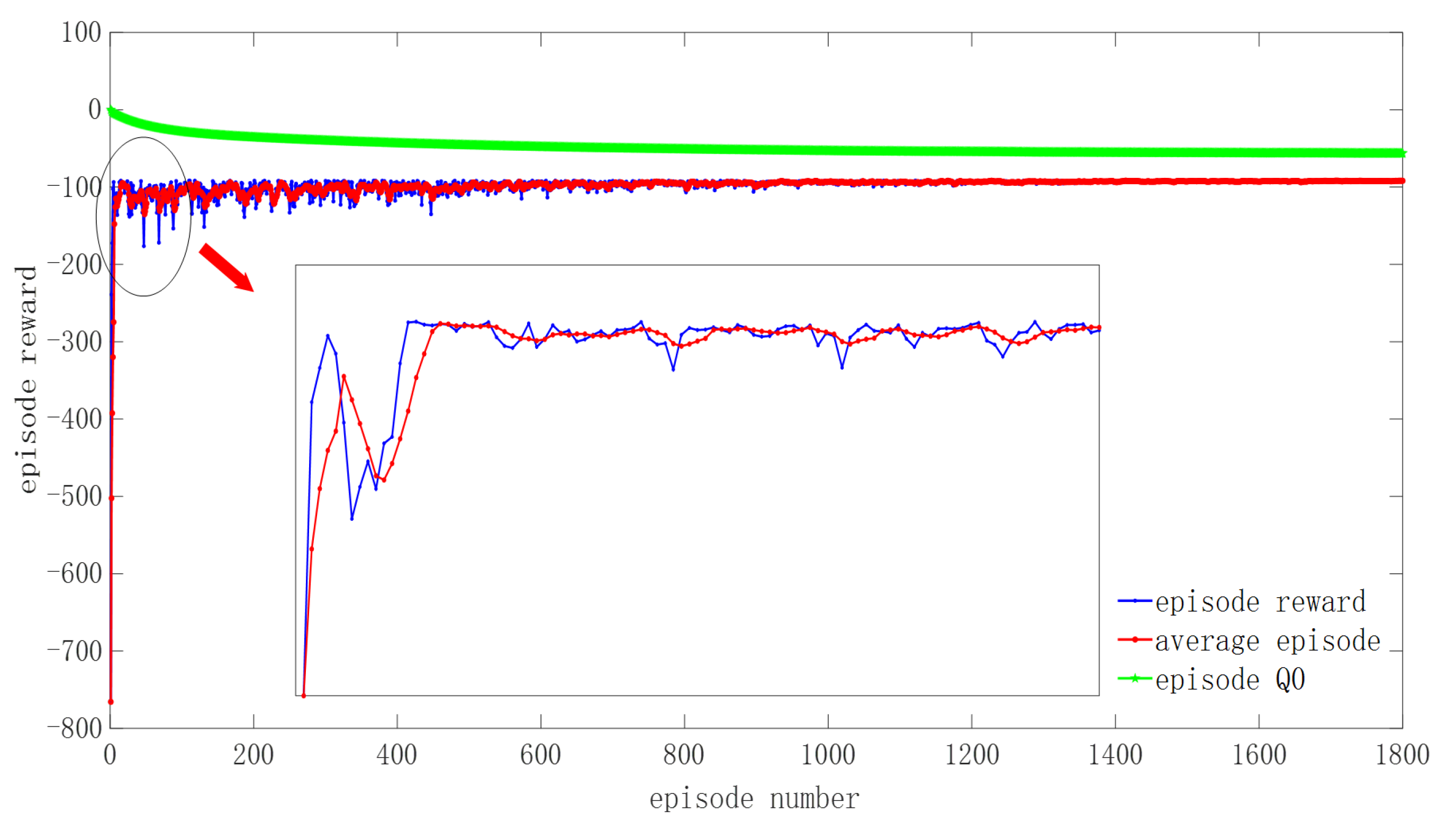
This simulation design is a single-point control precision simulation experiment. The sampling time is 0.02 s. Single episode time is 10 s, with a total of 1800 episodes. Two simulation experiments were designed. They involve the additive torque disturbance value $\left[\begin{array}{cc}1& 1\\ 1& 1\end{array}\right]$ and undisturbed value. The training progress is shown in Figure 7 and Figure 8.

In Figure 7 and Figure 8, the blue curve represents the change in the total reward value for each episode of training. The red curve represents the change curve of the average value of the total episode reward. The cyan curve is the Q value change curve for each episode of the evaluation network. With the increase in the number of training episodes, the fluctuation of the curve tends to be stable, the network finally converges, and the agent reaches the optimal value in this state. Overall, there is no difference between the two situations. Due to the anti-disturbance adjustment of the controller, the curve fluctuation is different in early training. It is proven that the DDPG controller has a strong anti-disturbance ability and strong stability.

Through the 2-joint experimental simulation of the snake manipulator, it is proven that the DDPG algorithm can improve the anti-interference and stability of the manipulator control system. Through many repetitions of training and learning, the position control accuracy of the end of the manipulator can be improved. However, it is difficult to establish the overall model of the snake manipulator. Thus, it is difficult to realize the model-based DDPG control method.

4. Control Simulation of Snake Manipulator Based on Data-Drive

According to the 2-link model, the dynamic model of the snake manipulator is complex and difficult to establish. The modeling of the whole snake manipulator not only is difficult but also involves a large number of parameters. According to the model-free data-driven control method, a data-driven control method based on DDPG is proposed for which an accurate snake manipulator and environment model are not required. This method avoids the influence of model uncertainty on the control system to improve the safety and reliability of the system.

4.1. Data Set Establishment

Since the snake manipulator mainly adopts the joint modular design method, as shown in Figure 3, according to the 2-link model of the snake manipulator, the overall 10-link snake manipulator model can be established. By using the traditional motion control method of the snake manipulator, the motion parameters of the snake manipulator are obtained. The data in the database are mainly based on the snake manipulator using the firework-optimized BP neural network PID (FWA-BPNN-PID) control method to perform varied trajectory motion. Part of the trajectory is shown in Figure 9.

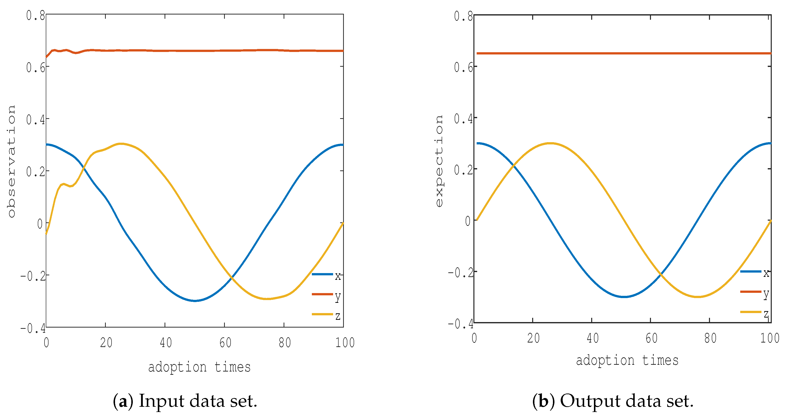
The data set of this simulation takes the origin as the center and 0.3 as the radius. The endpoint trajectory moves counterclockwise from the point (0.3), as shown in Figure 9a. Since the trajectory of the endpoint in the figure is designed on the plane of y = 0.65, the coordinate value y of the endpoint of the track is expected to remain the same. The coordinate values of the output result of the FWA-BPNN-PID method in Figure 9a are used as the input data set, and the sampling data are shown in Figure 10b. The desired track position coordinate values in Figure 9a are taken as the output data set, and the sampling data are shown in Figure 10b. The three curves in Figure 10 represent the values of the coordinate location in the data set.

4.2. Analysis of Simulation Results

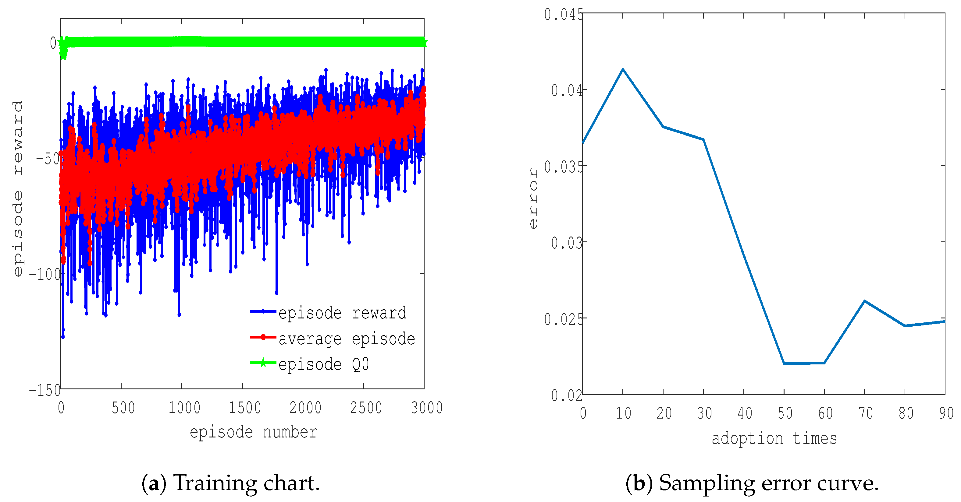
A new DDPG agent was built according to the method described in Section 3.3. The observed value of the agent is the coordinate position ${\left[\begin{array}{ccc}{x}_o& y_o& z_o\end{array}\right]}^{\mathrm{T}}$. The output action value is the coordinate location point ${\left[\begin{array}{ccc}{x}_a& y_a& z_a\end{array}\right]}^{\mathrm{T}}$. The reward value function is set to the error between the action value and the expected value. The sampling time of the training network is 1 s, the simulation time is 100 s, and the number of samples for a single episode is 100. The number of sample training episodes is set to 3000. The 3000 training results of the agent are shown in Figure 11. In Figure 11, it can be found that with the increase in training times, the reward value of the sample gradually tends toward zero, and the gap between the sample Q value and the sample Q value decreases and tends to be stable. When the sample reward value tends to be stable, it means that the system has converged and the network training has reached the current best state. The closer the sample reward value is to zero, the smaller the system error value is and the higher the system accuracy is.

The 12th, 1000th, and 3000 training states were randomly selected, and the error values are shown in

Table 2. Training error data of data-driven control method based on DDPG.

	FWA-BPNN-PID	12th	1000th	3000th
Average	0.0119	0.1420	0.0060	0.0034
MSE (${10}^{-5}$)	2.543	8.119	0.265	0.284

. The output results and error changes of the control system during training are shown in Figure 12.

Figure 12 shows the 12th training state in the initial stage, the 1000th in the middle of the training, and the 3000th at the end of the training. The three pictures on the left are error curves, which represent the data output error values for the database. The average errors of the 12th, 1000th, and 3000th training states are 0.0142, 0.006, and 0.0034, respectively. The specific data are shown in Table 2. The three pictures on the right side of Figure 12 are the output action graphs of the three training states, which clearly show that the curves become smoother and that the fluctuations are reduced. The fluctuation of the output curve represents the stability and accuracy of the output of the control system. With the increase in the number of training episodes, the stability of the system increases.

It can be found from Table 2 that, with the increase in training times, the control effect of the snake manipulator control system is better, and the control accuracy is continuously improved. In addition, compared with the traditional control methods, the control accuracy and stability of the snake manipulator control system are significantly improved, which verifies the effectiveness and superiority of the data-driven control algorithm based on DDPG.

4.3. Comparative Experimental Analysis

In order to test the influence of intelligent agent single-episode training times and agent network setting on the control system, a comparative experiment was designed. The first group of simulations is the original network, but the number of single-process training episodes is 10. The simulation results are shown in Figure 13. In the second group of simulations, the number of single training episodes is set to 10, and the agent action network adds a hidden layer. The hidden layer is set to the full connection layer, and the number of network nodes is set to 150. The simulation results are shown in Figure 14. The third group of simulations is based on the second group of experiments. The number of single training episodes is set to 100. The simulation results are shown in Figure 15.

As observed in Figure 13a, the training simulation chart converges slowly and fluctuates greatly compared with Figure 11. The average error of the sampling sample is 0.0301, and the Mean Square Error (MSE) is $4.7225\times {10}^{-5}$. Compared with the simulation of 100 samples, the average error and MSE are larger. This shows that the number of training samples is too small, which results in deterioration of the accuracy and stability of the control system.

When comparing the training chart of Figure 14a to the training chart of Figure 13a, we can observe that, after adding the network, the fluctuation value and convergence speed of the network do not change much. However, after increasing the network, the average error is 0.0271, and the MSE is $8.2381\times {10}^{-6}$. From numerical analysis, the increase in the number of network layers improves the accuracy and stability of the system.

By comparing the training chart of Figure 15a with that of Figure 11, it can be concluded that the convergence speed of the network is faster when the number of samples is the same. However, there are large fluctuations in the early stage, and the overall training time is longer. The average error value of 0.0061, and the MSE value of $1.1585\times {10}^{-6}$ can be obtained from the sampling error curve. Compared with the original network, the control accuracy of the simulation training system is reduced, but the stability is improved. The simulation results are shown in

Table 3. Comparison of simulation training error.

	Original	1st Group	2nd Group	3rd Group
Average	0.0034	0.0301	0.0271	0.0061
MSE (${10}^{-5}$)	0.284	4.7225	0.8238	0.1156

.

It can be observed from Table 3 that the number of samples and the number of network layers have an impact on the stability and accuracy of the system. Too few samples result in deterioration of the accuracy and stability of the control system. The control performance of the system can be improved by increasing the number of samples and training network layers. However, when the number of samples reaches a certain value, increasing the number of network layers can continue to improve the stability of the system. This, however, results in a decline in the accuracy of the system. In addition, increasing the number of samples and the number of network layers results in a longer training time of the system. In practical application, according to the needs of control, the number of samples of training or the number of network layers can be increased. This adjusts the manipulator control speed, stability, and accuracy to achieve a relative balance.

5. Summary and Prospects

In this study, the DRL algorithm was applied to a snake manipulator to verify whether it can improve its control accuracy. Through the study of the theory of DRL and the continuity of the action of the snake manipulator, the DDPG method is proposed as a means of designing the controller of the manipulator’s joint. A model-based DDPG control method is proposed to verify the effectiveness and superiority of the DDPG controller through the control of two joints, the simulation object environment and the network structure of the agent are established. The agent was trained, and the simulation without disturbance and torque disturbance was carried out. The simulation results verify the feasibility of the method. However, through the modeling of the 2-link snake manipulator, it was found that it is difficult to establish the entire manipulator model. It is difficult to realize the model-based DDPG control method for the whole manipulator control system. In order to solve the control problem of an unknown model of the snake manipulator, a data-driven control method based on DDPG is proposed. It does not need to establish an accurate manipulator model and avoids the influence of the accuracy error of the manipulator model. The training data were established according to the expected trajectory and the actual output trajectory of the traditional control method. Compared with the traditional control algorithm, it is proven that the data-driven control system based on DDPG has higher accuracy and better stability. At present, the control system of the snake manipulator is only based on data theory. In order to establish a complete snake manipulator motion library for training, the actual manipulator motion data and a large number of trajectory data are needed. The trained control system has a good ability to control known movements. For unknown actions, it also achieves a better control effect. By utilizing continuous learning, the strong adaptability of the snake manipulator control system can be realized.

References

- Hou, Z.; Xu, J. Review and prospect of data-driven control theory and method. J. Autom. 2009, 35, 650–667. [Google Scholar]
- Mendes, N.; Neto, P. Indirect adaptive fuzzy control for industrial robots: A solution for contact applications. Expert Syst. Appl. 2015, 42, 8929–8935. [Google Scholar] [CrossRef]
- Yen, V.; Nan, W.; Cuong, P.; Quynh, N.; Thich, V. Robust adaptive sliding mode control for industrial robot manipulator using fuzzy wavelet neural networks. Int. J. Control 2017, 15, 2930–2941. [Google Scholar] [CrossRef]
- Yen, V.; Nan, W.; Cuong, P. Recurrent fuzzy wavelet neural networks based on robust adaptive sliding mode control for industrial robot manipulators. Neural Comput. Appl. 2019, 31, 6945–6958. [Google Scholar] [CrossRef]
- Yu, X.; He, W. Research on adaptive neural network tracking control of manipulator based on disturbance observer. J. Autom. 2019, 45, 1307–1324. [Google Scholar]
- Jung, S. Improvement of tracking control of a sliding mode controller for robot manipulators by a neural network. Int. J. Control Autom. Syst. 2018, 16, 937–943. [Google Scholar] [CrossRef]
- Xia, M.; Zhang, X.; Weng, L.; Xu, Y. Multi-stage Feature Constraints Learning for Age Estimation. IEEE Trans. Inf. Forensics Secur. 2020, 15, 2417–2428. [Google Scholar] [CrossRef]
- Xia, M.; Wang, K.; Song, W.; Chen, C.; Li, Y. Non-intrusive load disaggregation based on composite deep long short-term memory network. Expert Syst. Appl. 2020, 160, 113669. [Google Scholar] [CrossRef]
- Xia, M.; Wang, K.; Zhang, X.; Xu, Y. Non-intrusive load disaggregation based on deep dilated residual network. Electr. Power Syst. Res. 2019, 170, 277–285. [Google Scholar] [CrossRef]
- Hasselt, H.; Guez, A.; Silver, D. Deep reinforcement learning with double q-learning. In Proceedings of the AAAI Conference on Artificial Intelligence, Phoenix, AZ, USA, 12–17 February 2016; pp. 1–13. [Google Scholar]
- Horgan, D.; Quan, J.; Budden, D.; Barth-Maron, G.; Hessel, M.; Hasselt, H. Distributed prioritized experience replay. 2018. Available online: https://arxiv.org/abs/1803.00933 (accessed on 6 August 2021).
- Wang, Z.; Schaul, T.; Hessel, M.; Hasselt, H.; Lanctot, M.; Freitas, N. Dueling network architectures for deep reinforcement learning. In Proceedings of the International Conference on Machine Learning, New York, NY, USA, 19–24 June 2016; pp. 1995–2003. [Google Scholar]
- Sutton, R.; Mcallester, D.; Singh, S.; Mansour, Y. Policy gradient methods for reinforcement learning with function approximation. Submitt. Adv. Neural Inf. Process. Syst. 1999, 99, 1057–1063. [Google Scholar]
- Barto, A.; Sutton, R.; Anderson, C. Neuron like elements that can solve difficult learning control problems. IEEE Trans. Syst. Man Cybern. 1970, 13, 834–846. [Google Scholar]
- Mnih, V.; Badia, A.; Mirza, M.; Graves, A.; Lillicrap, T.; Harley, T.; Kavukcuoglu, K. Asynchronous methods for deep reinforcement learning. In Proceedings of the International Conference on Machine Learning, New York, NY, USA, 19–24 June 2016; pp. 1928–1937. [Google Scholar]
- Weng, L.; Tian, L.; Hu, K.; Zang, Q.; Chen, X. Overview of robot force control algorithms based on neural network. In Proceedings of the 2020 Chinese Automation Congress (CAC), Shanghai, China, 6–8 November 2020; pp. 6800–6803. [Google Scholar]
- Levine, S.; Finn, C.; Darrell, T. End-to-end training of deep visuomotor policies. J. Mach. Learn. Res. 2016, 17, 1334–1373. [Google Scholar]
- Pinto, L.; Gupta, A. Supersizing self-supervision: Learning to grasp from 50k tries and 700 robot hours. In Proceedings of the 2016 IEEE International Conference on Robotics and Automation(ICRA), Stockholm, Sweden, 16–21 May 2016; pp. 3406–3413. [Google Scholar]
- Levine, S.; Pastor, P.; Krizhevsky, A.; Ibarz, J.; Quillen, D. Learning hand-eye coordination for robotic grasping with deep learning and large-scale data collection. Int. J. Robot. Res. 2018, 37, 421–436. [Google Scholar] [CrossRef]
- Lillicrap, T.; Hunt, J.; Pritzel, A.; Heess, N.; Erez, T.; Tassa, Y.; Wierstra, D. Continuous control with deep reinforcement learning. Comput. Ence 2015, 8, 1–10. [Google Scholar]
- Schulman, J.; Levine, S.; Abbeel, P.; Jordan, M.; Moritz, P. Trust region policy optimization. In Proceedings of the International Conference on Machine Learning, Lille, France, 6–11 June 2015; pp. 1889–1897. [Google Scholar]
- Luo, J.; Solowjow, E.; Wen, C.; Ojea, J.A.; Agogino, A. Deep reinforcement learning for robotic assembly of mixed deformable and rigid objects. In Proceedings of the 2018 IEEE/RSJ International Conference on Intelligent Robots and Systems (IROS), Madrid, Spain, 1–5 October 2018; pp. 1–5. [Google Scholar]
- Wu, X.; Zhang, D.; Qin, F.; Xu, D. Deep reinforcement learning of robotic precision insertion skill accelerated by demonstrations. In Proceedings of the 2019 IEEE 15th International Conference on Automation Science and Engineering (CASE), Vancouver, BC, Canada, 25–28 August 2019; pp. 1651–1656. [Google Scholar]
- Wen, S.; Chen, J.; Wang, S.; Zhang, H.; Hu, X. Path planning of humanoid arm based on deep deterministic policy gradient. In Proceedings of the 2018 IEEE International Conference on Robotics and Biomimetics (ROBIO), Kuala Lumpur, Malaysia, 12–15 December 2018; pp. 1755–1760. [Google Scholar]
- Wang, J.; Wang, G.; Mao, X.; Ma, Q. Motion control method of two-link manipulator based on deep reinforcement learning. Comput. Appl. 2021, 41, 1799–1804, (In Chinese with English Abstract). [Google Scholar]
- Li, Z.; Ma, H.; Ding, Y.; Wang, C.; Jin, Y. Motion Planning of Six-DOF Arm Robot Based on Improved DDPG Algorithm. In Proceedings of the 2020 39th Chinese Control Conference (CCC), Shenyang, China, 27–29 July 2020; pp. 3954–3959. [Google Scholar]
Figure 1.
DDPG network structure.
Figure 2.
Control block diagram based on DDPG control system.
Figure 3.
Structural model diagram of snake manipulator. (A) is the connecting rod structure and (B) is the universal joint structure.
Figure 4.
Joint coordinate system.
Figure 5.
Q network structure design.
Figure 6.
Action network structure design.
Figure 7.
Undisturbed training chart.
Figure 8.
Diagram of disturbance training.
Figure 9.
Partial trajectory motion diagram of snake arm in the database.
Figure 10.
Input and output data set.
Figure 11.
One hundred samples for a single episode and 3000 training maps for agents.
Figure 12.
Sampling of the system training process: (left) error curve; (right) output value.
Figure 13.
The first group of simulations.
Figure 14.
The second group of simulations.
Figure 15.
The third group of simulations.