
Analysis of the Scattering from a Two Stacked Thin Resistive Disks Resonator by Means of the Helmholtz–Galerkin Regularizing Technique


Department of Electrical and Information Engineering, University of Cassino and Southern Lazio, 03043 Cassino, Italy
Appl. Sci. 2021, 11(17), 8173; https://0-doi-org.brum.beds.ac.uk/10.3390/app11178173
Submission received: 15 August 2021
/
Revised: 30 August 2021
/
Accepted: 31 August 2021
/
Published: 3 September 2021
(This article belongs to the Special Issue Advances in Analytical-Numerical Techniques for Planar Microwave Circuits and Microstrip Antennas)
Abstract
:In this paper, the scattering of a plane wave from a lossy Fabry–Perót resonator, realized with two equiaxial thin resistive disks with the same radius, is analyzed by means of the generalization of the Helmholtz–Galerkin regularizing technique recently developed by the author. The disks are modelled as 2-D planar surfaces described in terms of generalized boundary conditions. Taking advantage of the revolution symmetry, the problem is equivalently formulated as a set of independent systems of 1-D equations in the vector Hankel transform domain for the cylindrical harmonics of the effective surface current densities. The Helmholtz decomposition of the unknowns, combined with a suitable choice of the expansion functions in a Galerkin scheme, lead to a fast-converging Fredholm second-kind matrix operator equation. Moreover, an analytical technique specifically devised to efficiently evaluate the integrals of the coefficient matrix is adopted. As shown in the numerical results section, near-field and far-field parameters are accurately and efficiently reconstructed even at the resonance frequencies of the natural modes, which are searched for the peaks of the total scattering cross-section and the absorption cross-section. Moreover, the proposed method drastically outperforms the general-purpose commercial software CST Microwave Studio in terms of both CPU time and memory occupation.
1. Introduction
The great interest in studying electromagnetic scattering from thin objects originates from the huge number of applications in which they are involved: frequency selective surfaces, antennas, radomes, tree leaves models, etc. More recently, the discovery of graphene [1], which is a planar monolayer of carbon atoms with amazing electronic, optical, thermal, and mechanical properties, and the consequent countless number of devices imagined to be made with such a material, have been leading to an impressive push towards the accurate study of lossy thin structures.
Boundary and radiation conditions together with the local power boundedness condition allow to formulate a uniquely solvable boundary value problem for the Maxwell equations, for which, in general, no closed form solutions are available, except for problems involving suitable canonical structures [2]. In other cases, only approximate solutions are provided based on Rayleigh–Gans or physical optics [3,4,5]. Consequently, the analysis of general structures or the search for more accurate solutions require the use of numerical methods. Amongst them, the classical Moments’ method approach is generally preferred because the unknowns and the integral equations are defined on finite supports, the radiation condition is automatically satisfied by the proper selection of the Green’s function of the problem and the local power boundedness condition is guaranteed by the correct definition of the functional space at which the unknowns belong.
Unfortunately, the discretization of a 3-D problem is generally onerous in terms of storage requirements. On the other hand, when the thickness is much smaller than the wavelength, the scatterer can be modelled as an infinitesimally thin structure described in terms of suitable generalized boundary conditions [6]. Just for an example, this is what happens when dealing with a graphene object, for which the surface impedance can be obtained from the graphene surface conductivity provided by the Kubo formalism [7]. According to this approach, the boundary value problem for the Maxwell equations at hand can be equivalently formulated in terms of a uniquely solvable system of 2-D singular integral equations for the effective surface current densities [8,9]. It is worth noting that, due to the singular nature of the obtained integral equations, nothing can be established a priori about the existence of the solution. Moreover, the convergence of the approximate solution, obtained by adopting a discretization scheme, to the exact one, if it exists, cannot be, in general, predicted [10]. Anyway, ill-conditioned and/or dense matrices can result from a direct discretization.
One way to overcome all these problems is represented by the methods of analytical regularization [11]. Such methods are aimed at individuating a suitable singular part of the integral operator, containing the most singular part of the operator itself, to be analytically inverted. The selection of such an operator depends on the problem at hand. Usually, it can be a suitable asymptotic part (e.g., the static part or the high-frequency part, etc.) or a canonical-shape part, which can be inverted by means of functional techniques such as Wiener–Hopf, Cauchy, Titchmarsh, Abel, Riemann–Hilbert Problem, and the separation of variables techniques [12,13,14,15,16,17,18,19,20]. Following this line of reasoning, the resulting integral equation is of the Fredholm second-kind; hence, the Fredholm theory [21], generalized by Steinberg for operators [22], can be applied. As a result, the existence originates from the uniqueness and the convergence of a discretization scheme preserving the Fredholm second-kind nature of the obtained integral equation is guaranteed. On the other hand, a proper choice of the discretization scheme can lead directly to a Fredholm second-kind matrix equation. This is what happens when: (1) the Galerkin scheme is adopted, and (2) the selected expansion functions are orthonormal eigenfunctions of a suitable operator containing the most singular part of the integral operator at hand. Such an approach, appropriately called method of analytical preconditioning, is very effective, as clearly shown in the literature devoted to the study of the scattering, propagation, and radiation problems [23,24,25,26,27,28,29,30,31,32,33]. Another way to obtain a guaranteed-convergence consists in solving numerically the singular integral equation by means of a Nyström-type discretization scheme taking into account the singularity of the integral equation and the behavior of the unknowns at the edges [34,35,36,37,38].
When dealing with thin disks, the complexity of the problem can be significantly reduced [39,40,41,42,43]. Indeed, the Fourier series expansion of the unknowns and the orthogonality property of the cylindrical harmonics allow recasting the surface integral equations as infinite sets of independent 1-D integral equations for the harmonics of the effective surface current densities. The strategy of combining the vector Hankel transform (VHT) [44] and the Helmholtz decomposition [45] is particularly suitable because the spectral domain counterpart of the surface curl-free and divergence-free contributions of the currents are scalar functions. After assuming such functions as new unknowns in the spectral domain, the method of analytical preconditioning can be readily applied. The selected expansion functions in the spectral domain, diagonalizing the most singular part of the integral operator, have a closed-form spatial domain counterpart reconstructing the behavior of the unknowns at the disk rim and around the centre of the disk. As a result, the projection integrals reduce to algebraic products and the convergence is very fast. Moreover, the 1-D improper integrals of the coefficient matrix can be quickly and accurately evaluated by adopting the analytical technique developed in [46] and generalized in [40].
In this paper, the method described above is successfully generalized to the analysis of a lossy Fabry–Perót resonator realized with two equiaxial thin resistive disks with the same radius. As will be clearly shown: (1) The proposed method is fast convergent and allows one to accurately and efficiently reconstruct both near-field and far-field parameters; (2) The resonance frequencies of the structure are simply individuated by the peaks of the total scattering cross-section (TSCS) and the absorption cross-section (ACS), which are expressed in closed form; (3) The proposed method drastically outperforms the general-purpose commercial software CST Microwave Studio (CST-MWS) in terms of both CPU time and memory occupation.
2. Formulation of the Problem and Proposed Solution
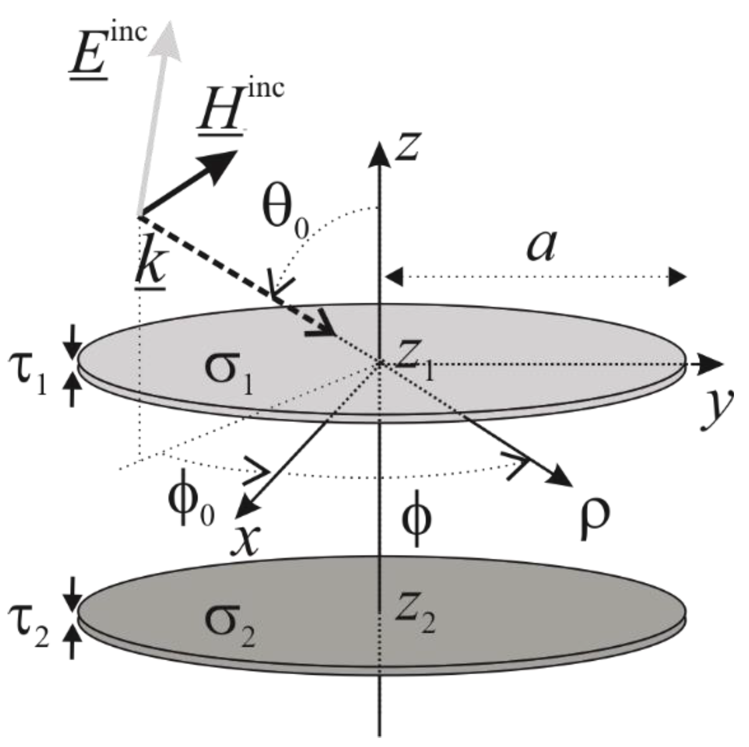
Two equiaxial resistive disks with the same radius a, thickness and electric conductivity , where identifies the i-th disk, in free space are considered (see Figure 1). A Cartesian coordinate system, , and a cylindrical coordinate system, , are introduced so that the z axis coincides with the axis of the disks and the median surfaces of the disks are located at the abscissas . Henceforth, the symbols , , , , , and will be used to denote the dielectric permittivity and magnetic permeability of free space, the frequency and the angular frequency, the wavelength, the free space wavenumber and intrinsic impedance, respectively. For high conductivity and thin disks, i.e., for , and , the disks can be approximated with infinitesimally thin flat surfaces located at the abscissas [6]. Effective surface current densities, , are excited on the disks by an impinging plane wave, and , where , , denote the unit vectors in the directions, respectively, and the incidence angles and are defined in Figure 1, which, in turn, generate scattered fields, , such that the overall scattered field satisfies the conditions .
A uniquely solvable boundary value problem for the Maxwell equations [8] is obtained by imposing the radiation condition, the local power boundedness condition and the following generalized boundary conditions on the disks [6]:
for , and , where denotes the total field and is the electric resistivity of the i-th disk.
It is well-known that the problem at hand can be equivalently formulated in terms of a system of 2-D integral equations for the effective surface current densities [9]. Moreover, the radiation condition can be automatically satisfied by the proper selection of the Green’s function of the problem whereas the local power boundedness condition is guaranteed by the edge behavior prescribed for the fields.
Taking advantage of the revolution symmetry of the problem at hand, the fields can be expanded in Fourier series, i.e.,
In this way, the orthogonality of the Fourier series terms allows to reduce the system of surface integral equations to an infinite set of independent systems of 1-D singular integral equations for the harmonics of the effective surface current densities. It is possible to show that the system of equations associated to the n-th harmonics of the currents can be written in the VHT domain as in the following:
for and , where the symbol is introduced to denote the column vector ,
is the VHT of order n (VHTn) of the n-th harmonic of the current on the i-th disk, is the kernel of the VHTn [44],
with is the spectral domain Green’s function of the problem at hand, is the Kronecker delta, is the identity matrix, and is the n-th harmonic of the incident electric field in the i-th disk plane.
By means of the Helmholtz decomposition, the n-th harmonic of the current on the i-th disk is replaced by the superposition of a surface curl-free contribution, , and a surface divergence-free contribution, [45]. This is an advantageous choice because it allows us to obtain scalar unknowns in the spectral domain. Indeed, it is simple to show that the VHTn of with are scalar functions [41], i.e.,
Now, the system of Equation (3), which cannot admit a closed form solution, has to be solved by resorting to a discretization scheme. It is important to note that fast convergence and analytical regularization can be simultaneously achieved by means of the Galerkin method providing suitable expansions of the unknowns.
In order to guarantee fast convergence, orthogonal bases of the functional spaces at which the unknowns belong are the best choice. Such spaces can be completely characterized by the edge behavior [47] and the behavior around the origin of the harmonics of the currents, and observing that the sources are off the disks:
for , , , where are well behaved functions.
By selecting the following expansion functions:
where is the Bessel function of the first kind [48], which are orthonormal functions on the interval with the weight function [49], it is possible to demonstrate that the complete and non-redundant Neumann series [50]
where is the general expansion coefficient, , , and , reconstruct the physical behavior in (8) [40].
On the other hand, by extracting the asymptotic behavior of the kernel for in (3),
the system of Equation (3) can be rewritten as in the following:
for and . The discretization of (12) by means of the Galerkin method with the expansions (10) leads to a matrix operator equation. It is simple to show that the matrix operator associated with the first term at the left-hand side of (12) is diagonal due to the orthonormality property of the expansion functions. The general element of the matrix operator associated with the second term at the left-hand side of (12) can be expressed as a linear combination of integrals of the kind
Looking at Formula (13), it is clear as the integrands of the integrals associated to the mutual contributions, i.e., for , have an asymptotic exponential decay related to the distance between the disks, . On the other hand, the elements for coincide with the ones obtained for a single resistive disk analyzed in [40]. Hence, following the same line of reasoning presented in [40], it can be shown that is a compact operator in . To conclude, the obtained matrix equation is of the Fredholm second-kind in because the free term has a bounded -norm [39,40].
3. Numerical Results
The aim of this section is the validation of the method proposed in Section 2.
The approximate solution obtained by truncating a Fredholm second-kind matrix equation converges to the exact solution of the problem as the truncation order increases. In principle, the accuracy of the solution is limited only by the machine precision; in practice, it depends on the accuracy in the numerical evaluation of the coefficient matrix. It will be shown in the following that the solution proposed in this paper, together with the analytical technique shown in [40] devised to efficiently evaluate the 1-D improper integrals of oscillating and algebraic decaying functions filling the coefficient matrix, makes it possible to accurately reconstruct the solution with very low CPU time and memory occupation. It is worth noting that all the simulations are performed by means of an in-house software code running on a laptop equipped with an Intel Core i7-10510U 1.8 GHz, 16 GB RAM.
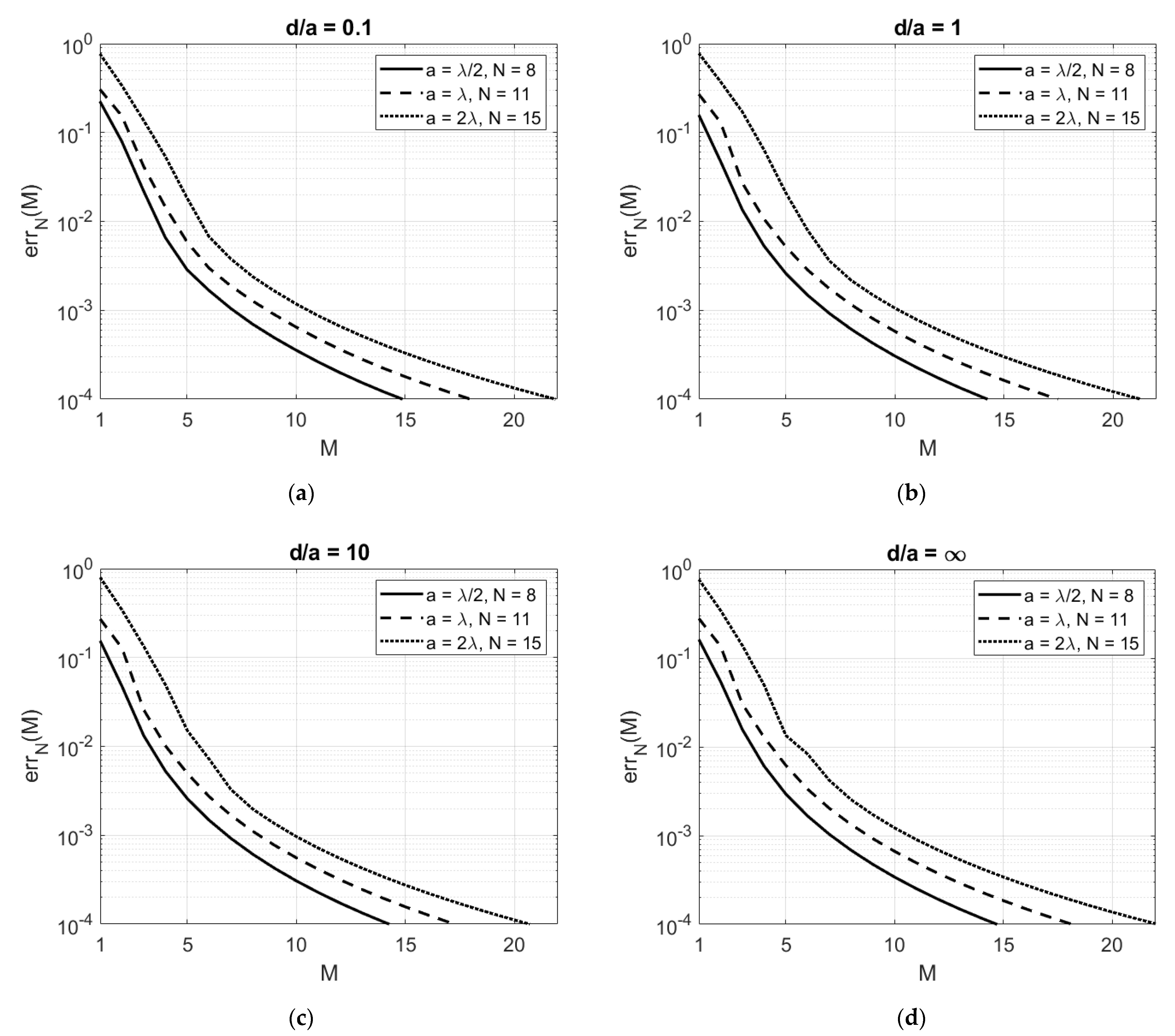
The rate of convergence will be analyzed by introducing the following relative computation error as a function of the truncation order of the matrix equation:
where is the number of cylindrical harmonics considered according to the estimation formula in [51], denotes the Euclidean norm, and is the vector related to the first M expansion coefficients of the general harmonics of the unknown functions.
Henceforth, it will be supposed that and (so that the distance between the disks could be changed by simply moving disk 2 along the z axis), and , , , , and transverse electric (TE) incidence with respect to the z axis.
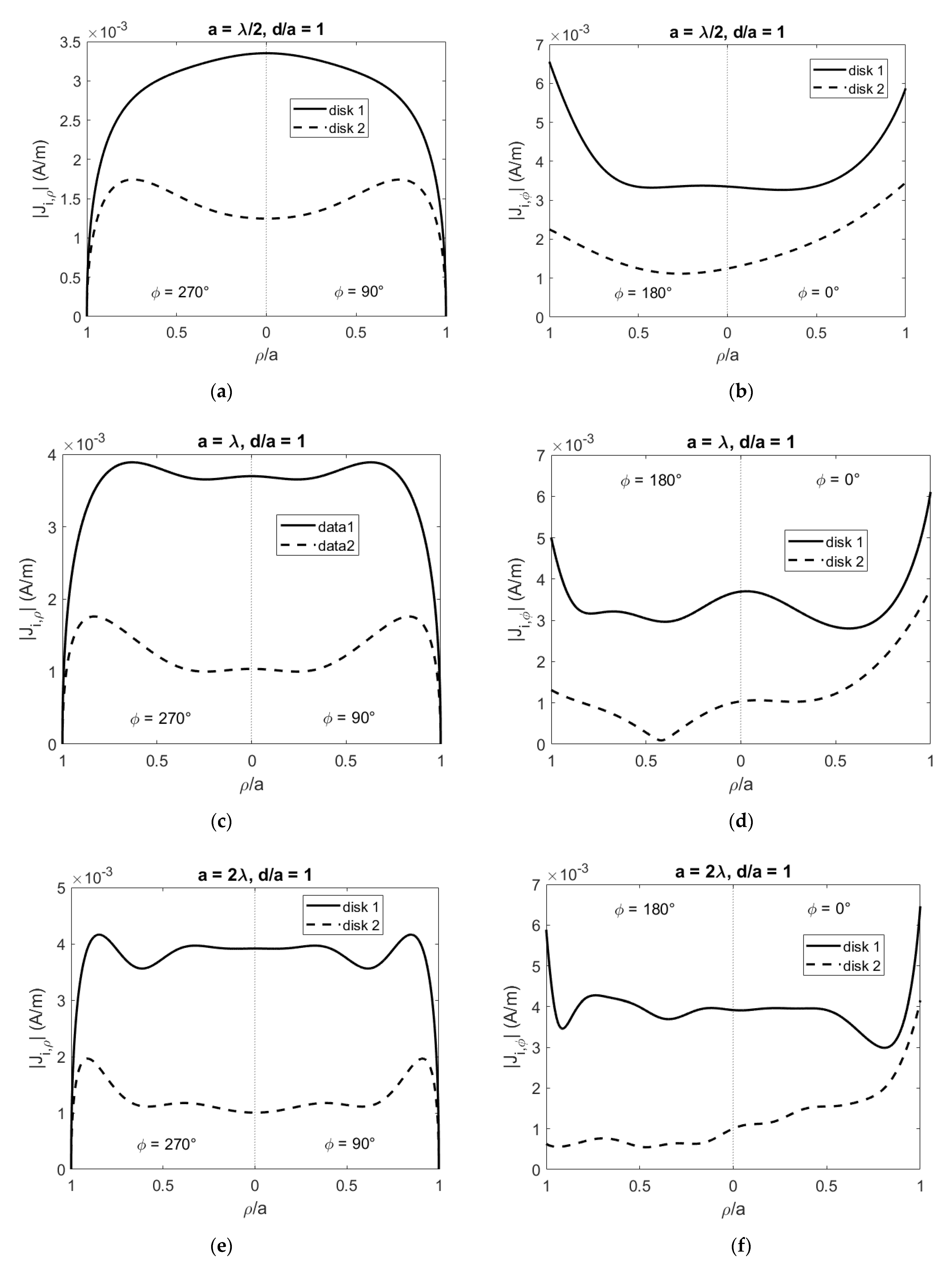
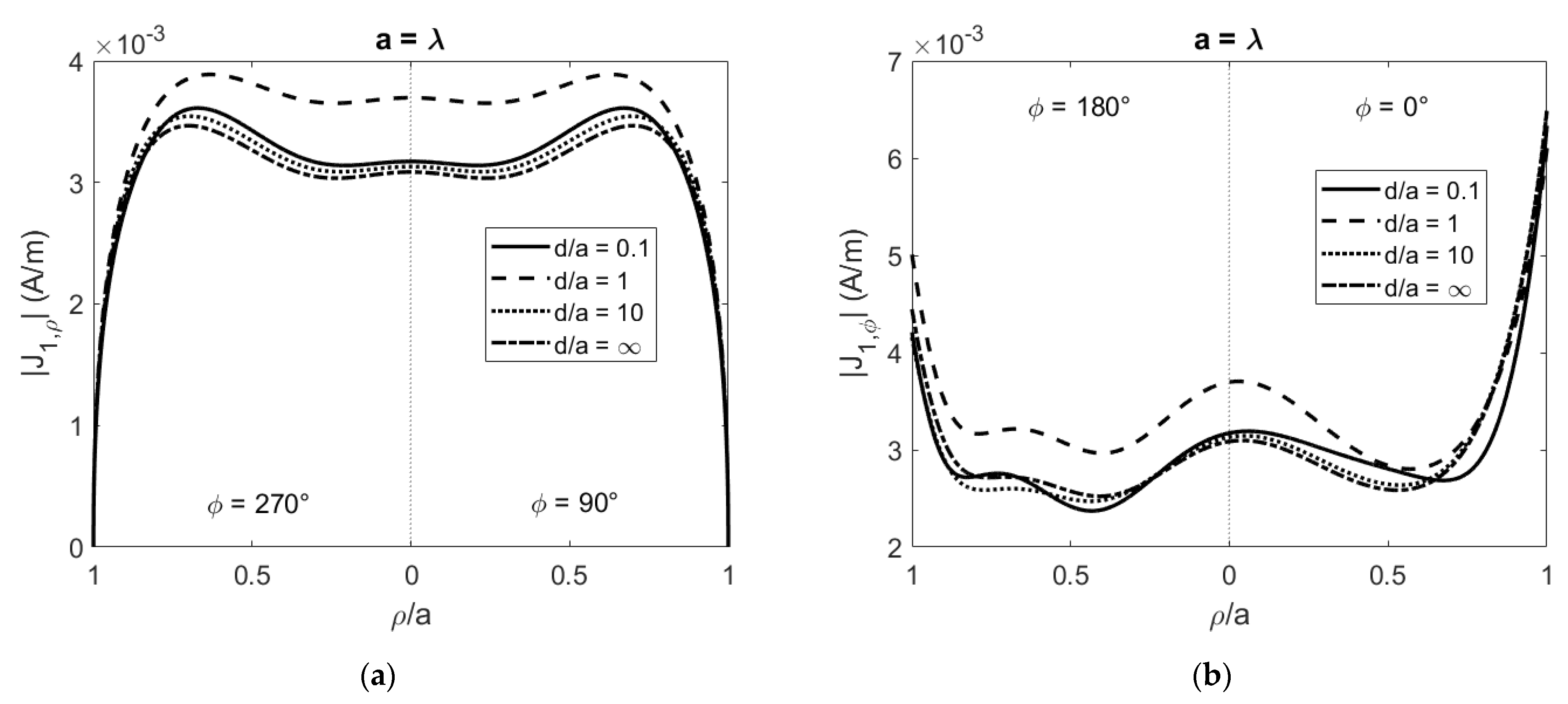
In Figure 2, is plotted for different values of the radius () and the distance between the disks (). As can be clearly seen, the error is substantially independent of the distance between the disks and it depends slightly on the radius of the disks in all the examined cases. It is apparent as the convergence is really very fast. Indeed, in the worst case examined ( and ), a relative error less than 1% is obtained for and with a computation time (t) of only 9 s. Moreover, more accurate solutions can be quickly obtained. Indeed, a relative error less than 0.1% and 0.01% is obtained for at most , and , , respectively. In the examples examined in the following M will be chosen in order to guarantee a relative error less than 1%. In Figure 3, for the sake of completeness, the reconstructed behavior of the components of the effective surface current densities for and for different values of the radius () is shown. Moreover, in Figure 4, the behavior of the components of the current on the disk 1, plotted for and for different values of the distance between the disks (), clearly shows that the proposed method tends to reconstruct the solution obtained in the case of a single disk () as the distance between the disks increases.
It is interesting to observe that the far scattered electric field can be expressed in closed form as a function of the unknowns in the spectral domain by means of the stationary phase method [9]:
with , where
As a result, the bistatic radar cross section (BRCS),
can be immediately evaluated once the solution of the problem is known.
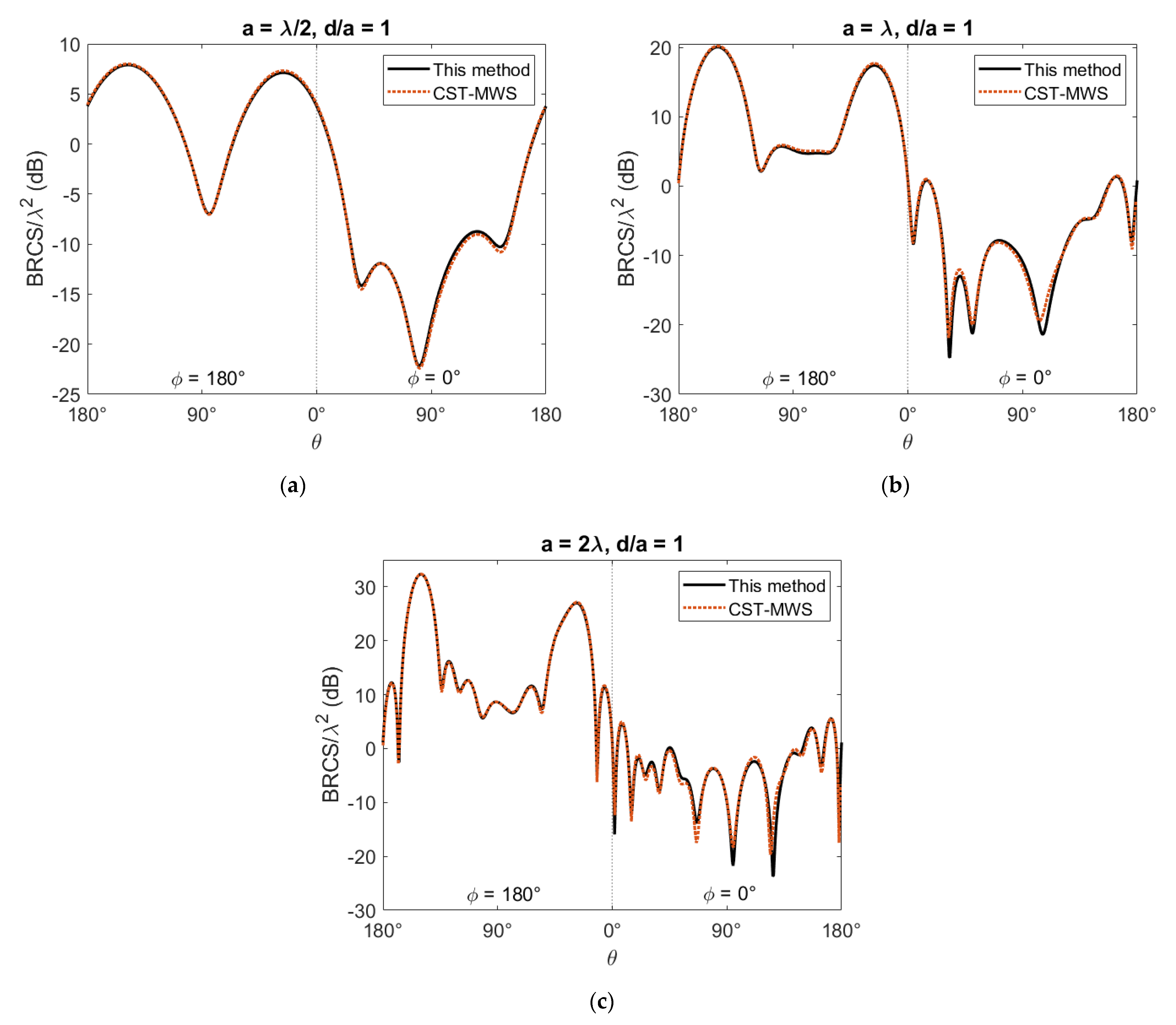
In Figure 5, BRCS is plotted for the cases considered in Figure 3, i.e., for and for . Comparisons with CST-MWS are provided for all the examined cases. As can be clearly seen, the agreement is really very good. However, the proposed method drastically outperforms the Integral Equation solver of CST-MWS, which requires tens of thousands of cells and a few minutes to find a reasonable approximation of the solution.
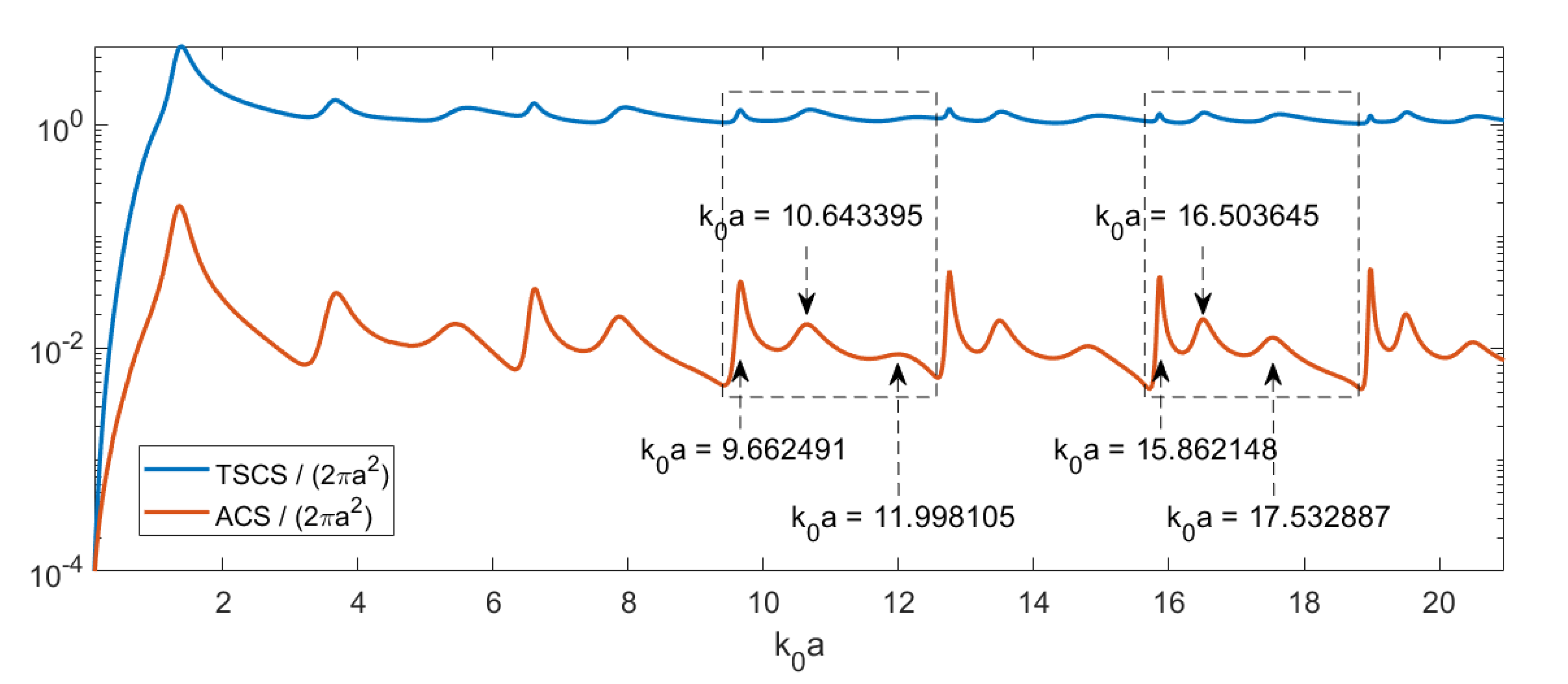
A resonant behavior can be observed due to the multiple reflection between the disks, i.e., the system of two stacked resistive disks works like a lossy Fabry–Pérot resonator. One way to individuate the resonance frequencies on the natural modes consists in searching for the peaks of TSCS and ACS, which are defined as in the following:
where is the power absorbed by the disks and denotes the real part of a complex number. As clearly shown in [43], by means of Parseval’s formula [52], Weber–Schafheitlin discontinuous integral [49] and forward scattering theorem [53], even TSCS and ACS can be expressed in closed form and then quickly evaluated.
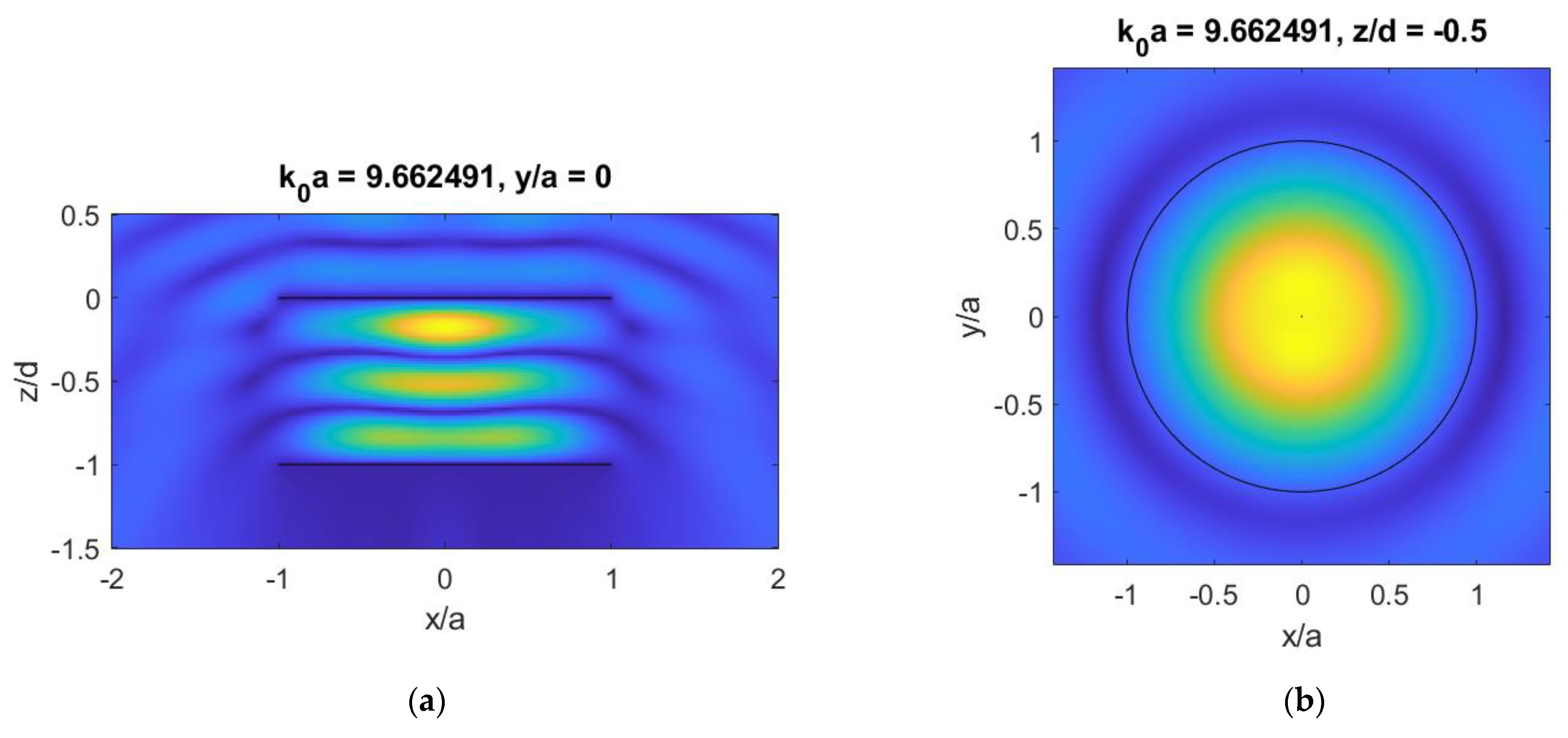
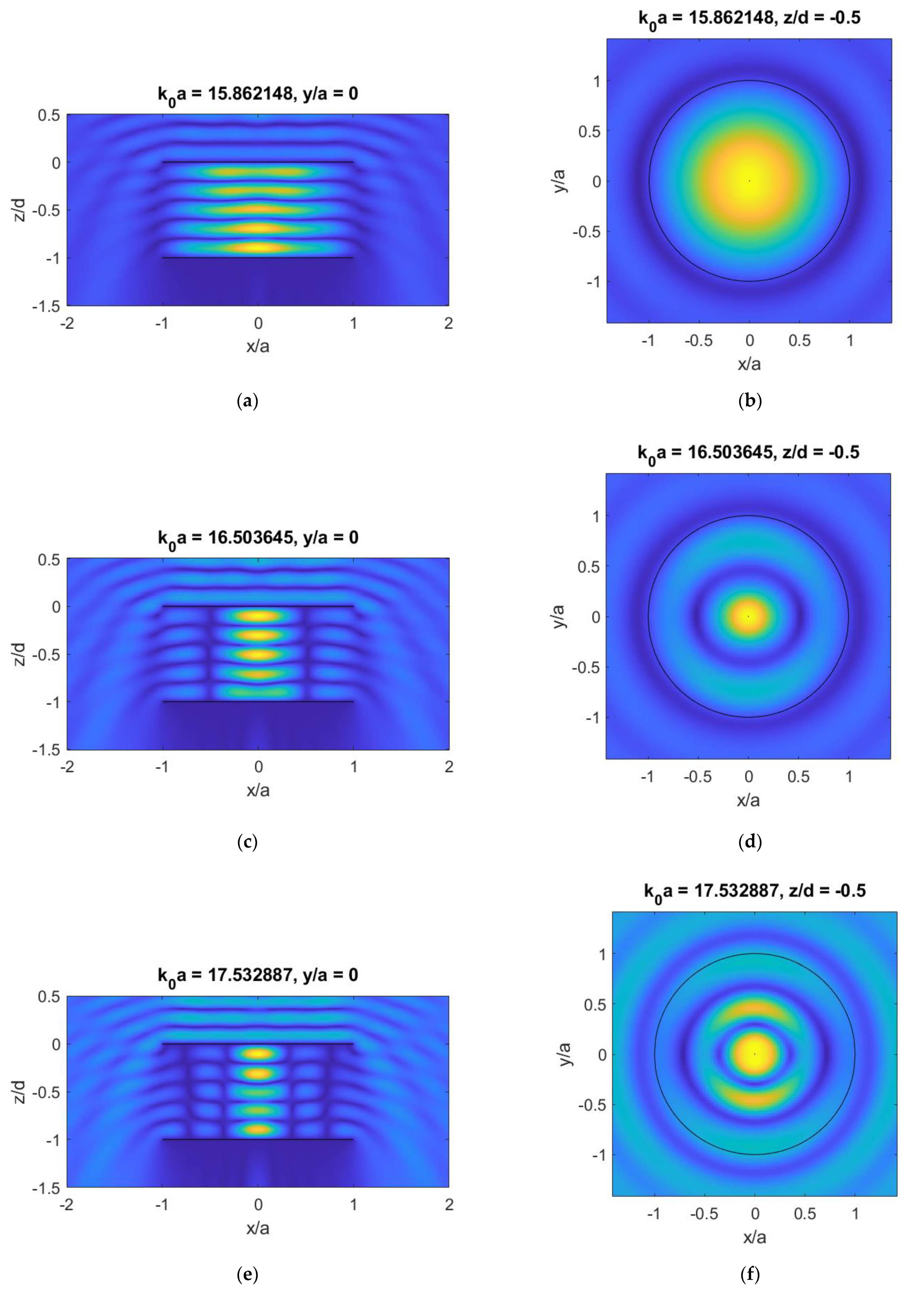
In order to clearly appreciate the resonant behavior of the proposed structure, it is assumed , i.e., the losses are reduced with respect to the cases examined above, providing the conditions for sufficiently high Q-factors of the resonant modes. Moreover, orthogonal incidence, i.e., , is considered so that only the harmonics for contribute to the representation of the solution. In Figure 6, TSCS and ACS for are plotted for varying values of the normalized frequency, . An almost periodic sequence of peaks can be clearly identified. In Figure 7 and Figure 8, the near E-field in the xz plane and plane is shown at the resonant frequencies in the two periods marked by the rectangular windows in Figure 6. It is interesting to observe that the field behavior is reconstructed by using at most 10 expansion functions for each unknown. Moreover, a given number of oscillations along the z axis is associated with each period, whereas the resonances in a period differ from each other by the number of oscillations along the radial direction. As expected, the resonances associated with the most pronounced peaks show a better confinement of the field between the disks.
4. Conclusions
In this paper, the analysis of the scattering from a two stacked thin resistive disks resonator has been successfully carried out by means of a generalized version of the Helmholtz–Galerkin regularizing technique recently developed by the author for the analysis of PEC, resistive/graphene, and dielectric disks. It has been clearly shown that the proposed method is accurate and efficient in reconstructing the near-field and the far-field parameters even at the resonance frequencies of the structure, and drastically outperforms CST-MWS. Future perspectives are the focus on the physical issues of the considered problem and the generalization of the proposed approach to the analysis of arrays of non-equiaxial resistive/dielectric/composite disks with different radii in both homogeneous and layered media.
Funding
This work was supported in part by the Italian Ministry of University program “Dipartimenti di Eccellenza 2018–2022”.
Institutional Review Board Statement
Not applicable.
Informed Consent Statement
Not applicable.
Data Availability Statement
The data presented in this study have been obtained by means of an in-house software code implementing the proposed method.
Conflicts of Interest
The author declares no conflict of interest. The funders had no role in the design of the study; in the collection, analyses, or interpretation of data; in the writing of the manuscript, or in the decision to publish the results.
References
- Geim, K.; Novoselov, K.S. The rise of graphene. Nat. Mater. 2007, 6, 183–191. [Google Scholar] [CrossRef] [PubMed]
- Senior, T.B.A.; Volakis, J.L. Approximate Boundary Conditions in Electromagnetics; Institution of Electrical Engineers: London, UK, 1995. [Google Scholar]
- Karam, M.A.; Fung, A.K.; Antar, Y.M. Electromagnetic wave scattering from some vegetation samples. IEEE Trans. Geosci. Remote Sens. 1988, 26, 799–808. [Google Scholar] [CrossRef] [Green Version]
- Koh, I.S.; Sarabandi, K. A new approximate solution for scattering by thin dielectric disks of arbitrary size and shape. IEEE Trans. Antennas Propag. 2005, 53, 1920–1926. [Google Scholar] [CrossRef] [Green Version]
- LeVine, D.M.; Schneider, A.; Lang, R.H.; Carter, H.G. Scattering from thin dielectric disks. IEEE Trans. Antennas Propag. 1985, 33, 1410–1413. [Google Scholar] [CrossRef] [Green Version]
- Bleszynski, E.; Bleszynski, M.; Jaroszewicz, T. Surface-integral equations for electromagnetic scattering from impenetrable and penetrable sheets. IEEE Antennas Propag. Mag. 1993, 35, 14–24. [Google Scholar] [CrossRef]
- Hanson, G.W. Dyadic Green’s functions for an anisotropic, non-local model of biased graphene. IEEE Trans. Antennas Propag. 2008, 56, 747–757. [Google Scholar] [CrossRef]
- Nosich, A.I. Method of analytical regularization in computational photonics. Radio Sci. 2016, 51, 1421–1430. [Google Scholar] [CrossRef]
- Jones, D.S. The Theory of Electromagnetism; Pergamon Press: New York, NY, USA, 1964. [Google Scholar]
- Dudley, D.G. Error minimization and convergence in numerical methods. Electromagnetics 1985, 5, 89–97. [Google Scholar] [CrossRef]
- Lucido, M.; Kobayashi, K.; Medina, F.; Nosich, A.I.; Vinogradova, E. Guest editorial: Method of analytical regularisation for new frontiers of applied electromagnetics. IET Microw. Antennas Propag. 2021, 15, 1127–1132. [Google Scholar] [CrossRef]
- Lovat, G.; Burghignoli, P.; Araneo, R.; Celozzi, S. Magnetic field penetration through a circular aperture in a perfectly conducting plate excited by a coaxial loop. IET Microw. Antennas Propag. 2021, 15, 1147–1158. [Google Scholar] [CrossRef]
- Kuryliak, D.B. The rigorous solution of the scattering problem for a finite cone embedded in a dielectric sphere surrounded by the dielectric medium. IET Microw. Antennas Propag. 2021, 15, 1181–1193. [Google Scholar] [CrossRef]
- Yevtushenko, F.O.; Dukhopelnykov, S.V.; Zinenko, T.L.; Rapoport, Y.G. Electromagnetic characterization of tuneable graphene-strips-on-substrate metasurface over entire THz range: Analytical regularization and natural-mode resonance interplay. IET Microw. Antennas Propag. 2021, 15, 1225–1239. [Google Scholar] [CrossRef]
- Oğuzer, T.; Altıntaş, A. Evaluation of the E-polarization focusing ability in Thz range for microsize cylindrical parabolic reflector made of thin dielectric layer sandwiched between graphene. IET Microw. Antennas Propag. 2021, 15, 1240–1248. [Google Scholar] [CrossRef]
- Tikhenko, M.E.; Radchenko, V.V.; Dukhopelnykov, S.V.; Nosich, A.I. Radiation characteristics of a double-layer spherical dielectric lens antenna with a conformal PEC disk fed by on-axis dipoles. IET Microw. Antennas Propag. 2021, 15, 1249–1269. [Google Scholar] [CrossRef]
- Vinogradova, E.D.; Smith, P.D. Scattering of an obliquely incident E−polarised plane wave from ensembles of slotted cylindrical cavities: A rigorous approach. IET Microw. Antennas Propag. 2021, 15, 1270–1282. [Google Scholar] [CrossRef]
- Vinogradova, E.D.; Kobayashi, K. Complex eigenvalues of natural TM-oscillations in an open resonator formed by two sinusoidally corrugated metallic strips. IET Microw. Antennas Propag. 2021, 15, 1283–1298. [Google Scholar] [CrossRef]
- Koshovy, G.I. The Cauchy method of analytical regularisation in the modelling of plane wave scattering by a flat pre-fractal system of impedance strips. IET Microw. Antennas Propag. 2021, 15, 1310–1317. [Google Scholar] [CrossRef]
- Doroshenko, V.O.; Stognii, N.P. Integral transforms and the regularisation method in the time-domain excitation of open PEC slotted cone scatterers. IET Microw. Antennas Propag. 2021, 15, 1360–1379. [Google Scholar] [CrossRef]
- Kantorovich, L.V.; Akilov, G.P. Functional Analysis, 2nd ed.; Pergamon Press: Oxford, UK, 1982. [Google Scholar]
- Steinberg, S. Meromorphic families of compact operators. Arch. Rational Mech. Anal. 1968, 31, 372–379. [Google Scholar] [CrossRef]
- Lucido, M. Scattering by a tilted strip buried in a lossy half-space at oblique incidence. Prog. Electromagn. Res. M 2014, 37, 51–62. [Google Scholar] [CrossRef] [Green Version]
- Corsetti, F.; Lucido, M.; Panariello, G. Effective analysis of the propagation in coupled rectangular-core waveguides. IEEE Photon. Technol. Lett. 2014, 26, 1855–1858. [Google Scholar] [CrossRef]
- Lucido, M.; Migliore, M.D.; Pinchera, D. A new analytically regularizing method for the analysis of the scattering by a hollow finite-length PEC circular cylinder. Prog. Electromagn. Res. B 2016, 70, 55–71. [Google Scholar] [CrossRef] [Green Version]
- Lucido, M.; Di Murro, F.; Panariello, G.; Santomassimo, C. Fast converging CFIE-MoM analysis of electromagnetic scattering from PEC polygonal cross-section closed cylinders. Prog. Electromagn. Res. B 2017, 74, 109–121. [Google Scholar] [CrossRef] [Green Version]
- Lucido, M.; Schettino, F.; Migliore, M.D.; Pinchera, D.; Di Murro, F.; Panariello, G. Electromagnetic scattering by a zero-thickness PEC annular ring: A new highly efficient MoM solution. J. Electromagn. Waves Appl. 2017, 31, 405–416. [Google Scholar] [CrossRef]
- Lucido, M.; Santomassimo, C.; Panariello, G. The method of analytical preconditioning in the analysis of the propagation in dielectric waveguides with wedges. J. Light. Technol. 2018, 36, 2925–2932. [Google Scholar] [CrossRef]
- Lucido, M.; Migliore, M.D.; Nosich, A.I.; Panariello, G.; Pinchera, D.; Schettino, F. Efficient evaluation of slowly converging integrals arising from MAP application to a spectral-domain integral equation. Electronics 2019, 8, 1500. [Google Scholar] [CrossRef] [Green Version]
- Lucido, M. Analysis of the propagation in high-speed interconnects for MIMICs by means of the method of analytical preconditioning: A new highly efficient evaluation of the coefficient matrix. Appl. Sci. 2021, 11, 933. [Google Scholar] [CrossRef]
- Fikioris, G. Regularised discretisations obtained from first-kind Fredholm operator equations. IET Microw. Antennas Propag. 2021, 15, 357–363. [Google Scholar] [CrossRef]
- Assante, D.; Panariello, G.; Schettino, F.; Verolino, L. Longitudinal coupling impedance of a particle traveling in PEC rings: A regularised analysis. IET Microw. Antennas Propag. 2021, 15, 1318–1329. [Google Scholar] [CrossRef]
- Assante, D.; Panariello, G.; Schettino, F.; Verolino, L. Coupling impedance of a PEC angular strip in a vacuum pipe. IET Microw. Antennas Propag. 2021, 15, 1347–1359. [Google Scholar] [CrossRef]
- Tsalamengas, J.L. Exponentially converging Nyström’s methods for systems of SIEs with applications to open/closed strip or slot-loaded2-D structures. IEEE Trans. Antennas Propag. 2006, 54, 1549–1558. [Google Scholar] [CrossRef]
- Nosich, A.A.; Gandel, Y.V. Numerical analysis of quasi-optical multireflector antennas in 2-D with the method of discrete singulari-ties. IEEE Trans. Antennas Propag. 2007, 55, 399–406. [Google Scholar] [CrossRef]
- Shapoval, O.V.; Sauleau, R.; Nosich, A.I. Scattering and absorption of waves by flat material strips analyzed using generalized boundary conditions and Nyström-type algorithm. IEEE Trans. Antennas Propag. 2011, 59, 3339–3346. [Google Scholar] [CrossRef]
- Kaliberda, M.E.; Lytvynenko, L.M.; Pogarsky, S.A.; Sauleau, R. Excitation of guided waves of grounded dielectric slab by a THz plane wave scattered from finite number of embedded graphene strips: Singular integral equation analysis. IET Microw. Antennas Propag. 2021, 15, 1171–1180. [Google Scholar] [CrossRef]
- Tsalamengas, J.L.; Vardiambasis, I.O. A parallel-plate waveguide antenna radiating through a perfectly conducting wedge. IET Microw. Antennas Propag. 2021, 15, 571–583. [Google Scholar] [CrossRef]
- Lucido, M.; Panariello, G.; Schettino, F. Scattering by a zero-thickness PEC disk: A new analytically regularizing procedure based on Helmholtz decomposition and Galerkin method. Radio Sci. 2017, 52, 2–14. [Google Scholar] [CrossRef]
- Lucido, M.; Schettino, F.; Panariello, G. Scattering from a thin resistive disk: A guaranteed fast convergence technique. IEEE Trans. Antennas Propag. 2021, 69, 387–396. [Google Scholar] [CrossRef]
- Lucido, M.; Balaban, M.V.; Dukhopelnykov, S.V.; Nosich, A.I. A fast-converging scheme for the electromagnetic scattering from a thin dielectric disk. Electronics 2020, 9, 1451. [Google Scholar] [CrossRef]
- Lucido, M. Electromagnetic Scattering from a Graphene Disk: Helmholtz-Galerkin Technique and Surface Plasmon Resonances. Mathematics 2021, 9, 1429. [Google Scholar] [CrossRef]
- Lucido, M.; Balaban, M.V.; Nosich, A.I. Plane wave scattering from thin dielectric disk in free space: Generalized boundary conditions, regularizing Galerkin technique and whispering gallery mode resonances. IET Microw. Antennas Propag. 2021, 15, 1159–1170. [Google Scholar] [CrossRef]
- Chew, W.C.; Kong, J.A. Resonance of nonaxial symmetric modes in circular microstrip disk antenna. J. Math. Phys. 1980, 21, 2590–2598. [Google Scholar] [CrossRef]
- Van Bladel, J. A discussion of Helmholtz’ theorem on a surface. AEÜ 1993, 47, 131–136. [Google Scholar]
- Lucido, M.; Di Murro, F.; Panariello, G. Electromagnetic scattering from a zero-thickness PEC disk: A note on the Helmholtz-Galerkin analytically regularizing procedure. Progr. Electromagn. Res. Lett. 2017, 71, 7–13. [Google Scholar] [CrossRef]
- Braver, I.; Fridberg, P.; Garb, K.; Yakover, I. The behavior of the electromagnetic field near the edge of a resistive half-plane. IEEE Trans. Antennas Propag. 1988, 36, 1760–1768. [Google Scholar] [CrossRef]
- Abramowitz, M.; Stegun, I.A. Handbook of Mathematical Functions; Verlag Harri Deutsch: Frankfurt, Germany, 1984. [Google Scholar]
- Gradstein, S.; Ryzhik, I.M. Tables of Integrals, Series and Products; Academic Press: New York, NY, USA, 2000. [Google Scholar]
- Wilkins, J.E. Neumann series of Bessel functions. Trans. Am. Math. Soc. 1948, 64, 359–385. [Google Scholar] [CrossRef]
- Geng, N.; Carin, L. Wide-band electromagnetic scattering from a dielectric BOR buried in a layered lossy dispersive medium. IEEE Trans. Antennas Propag. 1999, 47, 610–619. [Google Scholar] [CrossRef]
- Titchmarsh, E.C. Introduction to the Theory of Fourier Integrals; Oxford University Press: London, UK, 1948. [Google Scholar]
- Van Bladel, J. Electromagnetic Fields; IEEE Wiley: Hoboken, NJ, USA, 2007. [Google Scholar]
Figure 1.
Geometry of the problem.

Figure 2.
Relative computation error for a two stacked thin resistive disks resonator with different values of the radius of the disks () and of the distance between the disks (). , , , , , and TE incidence: (a) ; (b) ; (c) ; (d) .
Figure 2.
Relative computation error for a two stacked thin resistive disks resonator with different values of the radius of the disks () and of the distance between the disks (). , , , , , and TE incidence: (a) ; (b) ; (c) ; (d) .

Figure 3.
Components of the effective electric current densities on a two stacked thin resistive disks resonator for different values of the radius of the disks (). , , , , , and TE incidence: (a) , ; (b) , ; (c) , ; (d) , ; (e) , ; (f) , .
Figure 3.
Components of the effective electric current densities on a two stacked thin resistive disks resonator for different values of the radius of the disks (). , , , , , and TE incidence: (a) , ; (b) , ; (c) , ; (d) , ; (e) , ; (f) , .

Figure 4.
Components of the effective electric current densities on the upper disk (disk 1) of a two stacked thin resistive disks resonator for different values of the distance between the disks (). , , , , , , and TE incidence: (a) ; (b) .
Figure 4.
Components of the effective electric current densities on the upper disk (disk 1) of a two stacked thin resistive disks resonator for different values of the distance between the disks (). , , , , , , and TE incidence: (a) ; (b) .

Figure 5.
BRCS of a two stacked thin resistive disks resonator for different values of the radius of the disks (). , , , , , and TE incidence: (a) ; (b) ; (c) .
Figure 5.
BRCS of a two stacked thin resistive disks resonator for different values of the radius of the disks (). , , , , , and TE incidence: (a) ; (b) ; (c) .

Figure 6.
Normalized TSCS and ACS of a two stacked thin resistive disks resonator for varying values of the normalized frequency () when a plane wave orthogonally impinges onto the structure. , .
Figure 6.
Normalized TSCS and ACS of a two stacked thin resistive disks resonator for varying values of the normalized frequency () when a plane wave orthogonally impinges onto the structure. , .

Figure 7.
Near E-field behavior in the Cartesian coordinate planes xz and xy of a two stacked thin resistive disks resonator at three resonance frequencies (), when a plane wave orthogonally impinges onto the structure with : (a) Near E-field in the xz plane, ; (b) Near E-field in the xy plane, ; (c) Near E-field in the xz plane, ; (d) Near E-field in the xy plane, ; (e) Near E-field in the xz plane, ; (f) Near E-field in the xy plane, .


Figure 8.
Near E-field behavior in the Cartesian coordinate planes xz and xy of a two stacked thin resistive disks resonator at three resonance frequencies (), when a plane wave orthogonally impinges onto the structure with : (a) Near E-field in the xz plane, ; (b) Near E-field in the xy plane, ; (c) Near E-field in the xz plane, ; (d) Near E-field in the xy plane, ; (e) Near E-field in the xz plane, ; (f) Near E-field in the xy plane, .

Publisher’s Note: MDPI stays neutral with regard to jurisdictional claims in published maps and institutional affiliations. |
© 2021 by the author. Licensee MDPI, Basel, Switzerland. This article is an open access article distributed under the terms and conditions of the Creative Commons Attribution (CC BY) license (https://creativecommons.org/licenses/by/4.0/).
Share and Cite
MDPI and ACS Style
Lucido, M. Analysis of the Scattering from a Two Stacked Thin Resistive Disks Resonator by Means of the Helmholtz–Galerkin Regularizing Technique. Appl. Sci. 2021, 11, 8173. https://0-doi-org.brum.beds.ac.uk/10.3390/app11178173
AMA Style
Lucido M. Analysis of the Scattering from a Two Stacked Thin Resistive Disks Resonator by Means of the Helmholtz–Galerkin Regularizing Technique. Applied Sciences. 2021; 11(17):8173. https://0-doi-org.brum.beds.ac.uk/10.3390/app11178173
Chicago/Turabian StyleLucido, Mario. 2021. "Analysis of the Scattering from a Two Stacked Thin Resistive Disks Resonator by Means of the Helmholtz–Galerkin Regularizing Technique" Applied Sciences 11, no. 17: 8173. https://0-doi-org.brum.beds.ac.uk/10.3390/app11178173
Note that from the first issue of 2016, this journal uses article numbers instead of page numbers. See further details here.