
End-to-End Deep Reinforcement Learning for Image-Based UAV Autonomous Control

School of Automation Science and Electrical Engineering, Beihang University, Beijing 100083, China
*
Author to whom correspondence should be addressed.
Appl. Sci. 2021, 11(18), 8419; https://0-doi-org.brum.beds.ac.uk/10.3390/app11188419
Submission received: 2 August 2021
/
Revised: 4 September 2021
/
Accepted: 6 September 2021
/
Published: 10 September 2021
(This article belongs to the Special Issue Cutting-Edge Technologies of the Unmanned Aerial Vehicles (UAVs))
Abstract
:To achieve the perception-based autonomous control of UAVs, schemes with onboard sensing and computing are popular in state-of-the-art work, which often consist of several separated modules with respective complicated algorithms. Most methods depend on handcrafted designs and prior models with little capacity for adaptation and generalization. Inspired by the research on deep reinforcement learning, this paper proposes a new end-to-end autonomous control method to simplify the separate modules in the traditional control pipeline into a single neural network. An image-based reinforcement learning framework is established, depending on the design of the network architecture and the reward function. Training is performed with model-free algorithms developed according to the specific mission, and the control policy network can map the input image directly to the continuous actuator control command. A simulation environment for the scenario of UAV landing was built. In addition, the results under different typical cases, including both the small and large initial lateral or heading angle offsets, show that the proposed end-to-end method is feasible for perception-based autonomous control.
1. Introduction
In recent years, Unmanned Aerial Vehicles (UAVs) have been widely applied in various military and civil situations [1,2,3]. In particular, increasing attention has been paid to the autonomous control of UAVs [4]. UAVs are expected to fly safely on their own and make appropriate decisions without human intervention, completing their mission with higher efficiency and lower cost using entirely onboard sensing and computing. In missions of increasing complexity and uncertainty, it is becoming increasingly challenging for UAVs to react appropriately to dynamic environments in time.
The typical paradigm for achieving autonomous control is perception–planning–control. In this paradigm, the UAV first needs to observe the environment and determine its states relative to the environment with multiple sensors, including the exteroceptive information from the Global Positioning System (GPS) or the motion capture system, as well as the proprioceptive information from the Inertial Navigation System (INS) or visual sensors [5]. After perception, the UAV plans its trajectory or motion according to the optimization goal within various constraints [6]. Furthermore, low-level control commands are then generated for the inner loop controller in order to resolve commands hierarchically into signals for the actuator.
Schemes based on the perception–planning–control paradigm often consist of well-defined separate modules with the interfaces among them requiring appropriate handcrafted designs. However, these specifically designed interfaces may cause the intermediate representation to be restrictive and less adaptive to uncertainty. In addition, the unidirectional paradigm may lead to the accumulation of errors from different modules. Additionally, it is always necessary to build a prior model. On the one hand, the models are an idealized approximation and many significant effects are often omitted or cannot be accurately modeled [4]. On the other hand, it is difficult for model-based algorithms to deal with unknown system dynamics. When it comes to implementation, complicated algorithms such as mapping [7], estimation and online optimization [8] have a high computation cost, which is challenging for onboard micro-computers to meet.
Machine learning techniques have been widely used to provide robust and adaptive performance, while simultaneously reducing the required development and deployment time [9]. In particular, deep learning (DL) plays an essential role in various fields of study due to its capacity for extracting representative features of the input data by learning. It gives a possible solution for replacing handcrafted features with deep-learned features. Furthermore, the combination of DL with another branch of machine learning named reinforcement learning (RL), which depends on interaction with the environment, has demonstrated superiority in tasks with respect to both perception and decision making. Typical applications of deep reinforcement learning (DRL) methods include playing games [10,11], natural language processing [12,13], autonomous driving [14,15], robotics manipulation [16,17], and so on. Inspired by the idea of DRL, which integrates the feature representation ability of DL and the intelligent decision ability of RL, this paper proposes a UAV autonomous control framework based on end-to-end DRL with the image as the only input.. Unlike several previous works that produce discrete action [18] or reference velocity [19], a single deep neural network is established to map the input image directly onto the continuous actuator control command, and is trained with a reinforcement learning algorithm.
The main contributions of this paper include:
- A new solution based on end-to-end learning for the autonomous control of UAVs is proposed, which simplifies the traditional modularization paradigm by establishing an integrated neural network, directly mapping the image input of the onboard camera onto the low-level control commands of the actuators;
- An image-based reinforcement learning algorithm is implemented with the designed neural network architecture and the reward functions according to the specific scenario;
- The proposed method is validated on the basis of a UAV landing simulation under different cases with ROS and Gazebo. The results show that the end-to-end method allows the UAV to learn to land on the centerline of the runway even with large initial lateral and heading angle offsets.
The remainder of this paper is organized as follows. Section 2 details some representative related work. Preliminaries are presented in Section 3, including the problem statement. In Section 4, the proposed method is detailed from the aspects of the framework, network architecture, reward function and algorithm implementation. Then, the simulation experiments are described and discussed in Section 5. Finally, Section 6 summarizes this paper and gives some tips for future work.
2. Related Work
Traditional autonomous UAV control schemes are mostly based on the perception–planning–control framework. Ref. [20] focused on vision-based human following, wherein the researchers used a Haar cascade classifier to first detect the human face and track it with a Kalman filter. Then, the coordinate transformation was calculated to attain a pose estimation. In addition, an appropriate distance was maintained between them by using a linear PD controller. Ref. [21] proposed a system for the landing of a fixed-wing UAV comprising a vision module, a range finder (Lidar), and a high-precision aircraft controller. In addition, data from different sources are fused according to various phases. For quadrotor landing on a moving platform, [22] proposed a full-stack solution based on state-of-the-art computer vision algorithms, multi-sensor fusion for localization of the robot, detection and motion estimation of the moving platform, and path planning for fully autonomous navigation. An image-based visual servo controller was proposed in [23] for quadrotor vertical takeoff and landing of an unmanned aerial vehicle (UAV). The controller utilized an estimate of the flow of image features as the linear velocity cue and assumed angular velocity and attitude information available for feedback. In [24], binocular stereo vision was applied to perceive obstacles and the power lines to be inspected. In addition, the real-time local optimal path was then planned by combining the interfered fluid dynamical system (IFDS) method with the rolling optimization strategy. Ref. [25] formulated the position-based visual servo problem for a quadrotor equipped with a monocular camera and an IMU relying only on features on planes and lines in order to fly above and perch on arbitrarily oriented lines. Ref. [26] proposed a trajectory generation method for crossing narrow gaps in consideration of geometric, dynamic, and perception constraints. In addition, it also estimated the full state by fusing gap detection from a single onboard camera with an IMU. Similar methods were also discussed in [27,28,29] with respect to quadrotors equipped with VINS (visual-inertia navigation system), achieving safe flight through cluttered environments on the basis of the mapping module, the online trajectory planner, and the cascade controller. Ref. [30] provided a scheme for autonomous UAV guidance in a precision agriculture scenario based on image processing techniques. Crop row detection was performed on the basis of the Hough transformation to identify the line representing the crop row. Then, a line follower algorithm was designed to generate the trajectory for tracking the UAV.
With the development and application of machine learning and neural networks, direct mapping between perception and control can be established, making the sensorimotor control system more intelligent, including in the context of autonomous control of UAVs. Ref. [31] used only a single camera to perceive the environment and train a reactive controller on the basis of imitation learning in accordance with demonstrations by a human pilot in order to avoid obstacles in a cluttered environment. By virtue of the DAgger technique, the reactive control policy mapped the visual features directly to the left or right velocity control input. In addition, the experimental results showed that under the trained policy, the UAV was able to fly through dense forest at a velocity of up to 1.5 m/s. Ref. [2] focused on the problem of learning UAV autonomous control for the purpose of tracking a moving target. A neural network consisting of convolutional layers and fully connected layers was used to generate the control command on the basis of the image input. In addition, a hierarchical approach combining a model-free policy gradient method with a conventional feedback controller was proposed. In [32], a fast eight-layer residual network named DroNet was proposed to safely drive the UAV through the streets of a city. The network took the forward image as a single input and produced the steering angle and the collision probability as the output. In addition, it was trained by imitating expert behavior, which was generated from wheeled manned vehicles. To perform object following, [18] applied reinforcement learning in classical image-based servo control. The state inputs were the error of the center of the detected ROI and their derivatives. The output actions were the linear velocity commands sent to the velocity controller of the UAV. Under a similar scenario, the neural network used in [19] mapped the input RGB image onto discrete action. Additionally, the results of a tracking filter were added to the network to increase the robustness of the system.
As can be seen from the previous literature, some efforts have been made to tackle UAV autonomous control by training deep neural networks on the basis of feature input and command output, rather than basing them on separate modules in a traditional framework. Learning direct control policies from raw images to low-level continuous control commands is still an open issue. This paper further explores it via deep reinforcement learning with an end-to-end framework.
3. Preliminaries
3.1. Reinforcement Learning
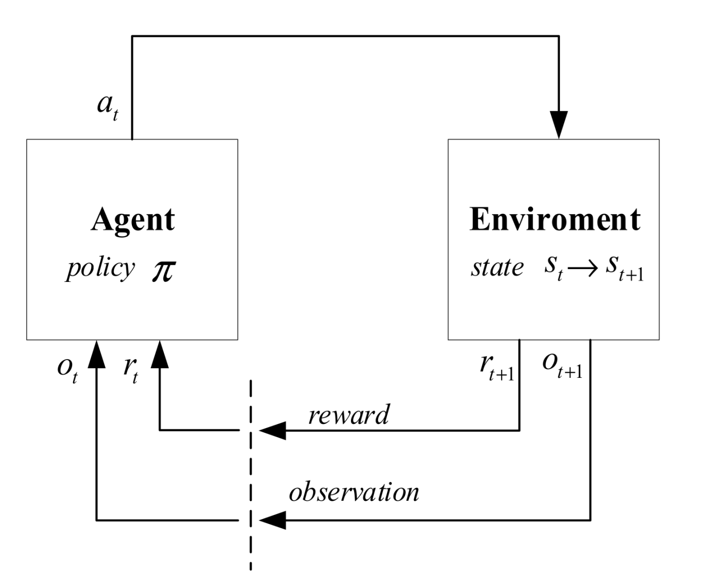
Reinforcement learning (RL) is suitable for sequential decision problems, in which the previous states and actions have an influence on the following states. Mathematically, this problem can be abstracted as a Markov decision process (MDP). As shown in Figure 1, an agent is defined to interact with an environment in a general RL problem. At each step, the RL-agent receives the observation and the reward from the environment and then produces an action according to a policy , which maps states to a probability distribution over the actions. Under the action , the environment shifts from state to and gives a new reward and the updated observation . Generally, the states of the environment are partially observable. However, can be assumed for a simple scenario, as well in this paper. The goal for the RL-agent is to interact with the environment and learn the optimal policy , maximizing the accumulated future reward called return , where is the terminal time step and is the discounting factor representing the influence of the subsequent rewards.
Based on the expectation of return , two types of value function are introduced to evaluate a policy: the state value function and the state-action value function . The commonly used is also known as the Q-function, and represents the expected return after taking action in state and thereafter following policy . Then, the optimal policy should satisfy .
3.2. Problem Formulation
For perception-based control problems, the UAV should generate proper control commands according to observations at each time. In addition, the state of the UAV is then updated to acquire new observations and produce new commands, until the goal is achieved. This process can be abstracted into a sequential decision problem. Therefore, RL could be one available solution. In this paper, the autonomous landing of a fixed-wing UAV with a down-view monocular camera is used as an example scenario. In addition, it can be regarded as an image-based RL problem. With respect to the description in Section 3.1, the only observed state in our problem is the image of the onboard camera (), and the action is an m-dimensional vector of control commands for the actuators (), such as the elevator, the ailerons, the rudder, the throttle, and the flaps. Under this concrete scenario, the goal is to have the UAV learn to land from a certain starting position on the centerline of the runway. To achieve this, an RL-agent for policy optimization needs to be trained to calculate the control commands according to the camera image at each moment.
4. Proposed Method
4.1. Framework
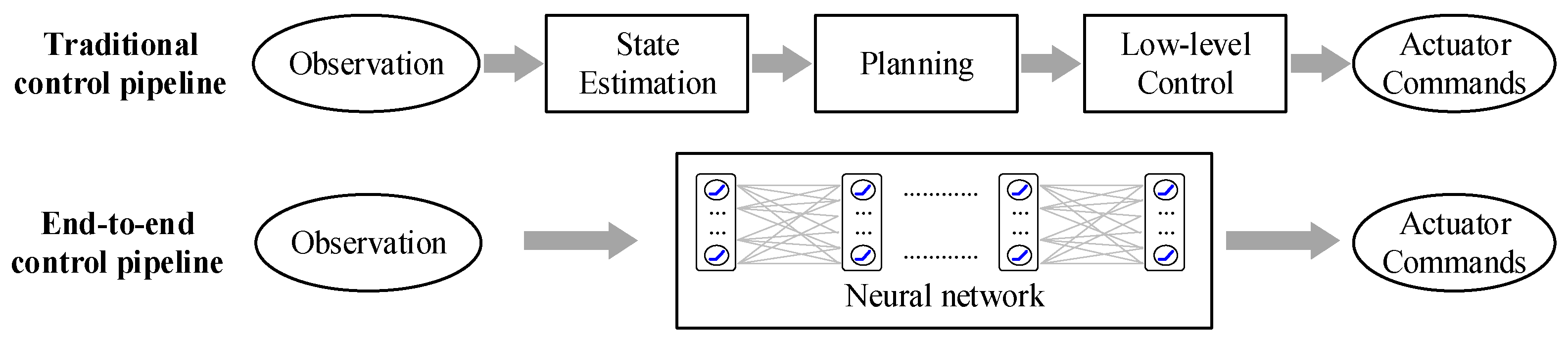
In Figure 2, the traditional control pipeline is presented, along with its modularization. To obtain the actuator commands on the basis of observation, usually, the state estimation, planning, and low-level control stages need to occur. This requires a series of independent modules, and the interfaces between different modules need to be handcrafted. By comparison, our proposed method is based on the end-to-end control pipeline. The core idea is to establish a direct mapping between the input-end (observation) and the output-end (actuator commands) of the system on the basis of the neural network. The end-to-end control pipeline simplifies the control process and is expected to autonomously extract the features that are supportive to the generation of the proper control commands.
Specific to the UAV control instance presented in this paper, the problem was abstracted as an image-based reinforcement learning problem in Section 3.2. To apply the proposed end-to-end control pipeline, the policy for the RL-agent is approximated by a neural network. To obtain the continuous action, the deep deterministic policy gradients (DDPG) algorithm with the actor-network and the critic-network is adopted. Therefore, the UAV perception-based control problem can be described in the image-based RL framework, as shown in Figure 3. Apart from the DDPG agent, the environment mainly consists of the external environment and the UAV model. The interaction between the two main parts is achieved by the environment interfaces, including the onboard camera and the reward function. The former is used to obtain the monocular image and the latter calculates the reward according to the control commands and UAV states. The raw image from the camera is an RGB image with a size of 640 × 480. In consideration of computational efficiency, it needs to be resized and converted to greyscale by the image processor.
4.2. Network Architecture
In general, the training of a neural network can be affected by various aspects, especially the network architecture including the number of the network layers, the structure of each layer, the selection of the activation function and so on. As the number of network layers increases, the complexity of the architecture may be beneficial for identifying complex features. However, the variation of input distribution resulting from the subtle changes in the parameters at each layer may be amplified layer by layer and the upper layer network has to adapt continuously to these distribution changes, increasing the difficulty of training. Additionally, different structures of each layer have their own properties. For instance, the fully connected network can be used to fuse the features, the convolutional network is used to extract the spatial features, and the recurrent network is appropriate for temporal sequence processing. The activation functions result in non-linearity, improving the representational ability of the network. In addition, their selection in each layer is related to the attributes of the input and output of the layer.
The architectures of the neural network designed for the DDPG agent in this paper are shown in Figure 4. The input and the output variables are noted in blue. The actor and the critic have a similar network architecture that consists of convolution layers and fully connected layers. The inputs of both of the networks consist of the pre-processed grey image from the downwards camera with the size of 128 × 128. To extract the features of the runway from the whole scene, 3 convolutional layers are used with max-pooling and the ReLU activation function. The size of the filter in each layer is 5 × 5. To reduce computation, the stride is set as 2. The output of the convolutional layers is finally given to the fully connected layer and then activated by tanh function for the output layer to keep the control commands within a fixed range. For the actor-network, its output is an m-dimensional vector in which each element corresponds to the control command of the respective actuators. The value of m is determined according to the specific mission and controlled object. For the critic-network, the current action vector is used as an additional input for the fully connected layer. In addition, its output is activated with ReLU function to produce a scalar that represents the estimated Q-value.
4.3. Reward Function
The design of the reward function is essential for an RL problem, and can influence the convergence of the algorithm. At each time instant, the RL-agent is encouraged to select the action that can provide the largest reward. To some extent, the reward function is supposed to give a positive response when the RL-agent makes a good decision. On the contrary, it gives a negative response to actions that mislead the RL-agent or violate the rules. Taking the landing of the fixed-wing UAV as an example, the UAV should decrease its height along the glide slope towards the centerline of the runway within a certain region. Therefore, the basic rules are not crossing the position border, including the height constrained by the glide slope and the lateral range confined by the geographic fence. Additionally, the attitude of the UAV should also be confined within a certain range to achieve stable and safe flight. For example, the pitch angle may be related to the maximum allowed attack angle to prevent stalling. These border-crossing conditions are judged to be an abnormal part of the reward and they are considered by giving a negative penalization value to inform the RL-agent of the constraints of the mission. Additionally, it is also necessary to encourage the RL-agent when it makes efforts to get closer to the goal of landing. It is hard to explicitly judge whether the current action is beneficial to the final success of landing. Here, these positive rewards are regarded as the normal part, and their values are determined according to the current pose of the UAV and its desired landing pose. Specifically, the desired lateral distance, height and yaw angle of the UAV when it lands right in the centerline of the runway are expected to be 0. In order to distinct from the negative reward, the bias term is added when calculating the positive reward to increase its baseline.
From the above, both the normal and abnormal parts are considered in the design of the reward function, as shown in Equation (1):
where is the distance error along the x-axis, are the lateral and vertical coordinates of the UAV, is its yaw angle, are constant parameters. represents the square error, and represents the absolute value. The normal part describes the approaching degree to the terminal landing state. The abnormal parts respectively indicate the constraints condition for the position and the attitude of the UAV.
4.4. Algorithm Implementation
To train the RL-agent, the image-based RL framework is developed with the DDPG algorithm, which is a kind of DRL, as an extension of deep Q-network algorithms. In contrast to deep Q-network algorithm, DDPG is based on the actor–critic framework, in which the critic is a parameterized function for estimating the Q-value, and the actor uses the parameterized function to approximate the optimal policy. Additionally, it can operate over continuous action spaces. On the one hand, DDPG algorithm introduces a deep neural network to approximate the critic function and the actor function, respectively, as a value network and a policy network, which makes processing high-dimensional and complex representations possible. On the other hand, it refers to the techniques of the deep Q-network algorithm named experience replay and target network in order to improve the stability of learning. Therefore, DDPG algorithm is proper for the image-based RL problem because it can resolve the image feature and generate the continuous control commands.
With the designed network architecture and the reward function, the DDPG algorithm can be implemented for the image-based autonomous landing task, and its diagram is shown in Figure 5. In the figure, arrows with different colors represent the data flow during different phases of the algorithm. In the beginning, the parameters of the networks are randomly initialized. The UAV starts from the designated initial position with certain velocity and attitude.
In each episode, the agent starts with a random exploration phase. The DDPG agent receives the processed image from the UAV and gives the action based on the current actor. Then an instant reward can be calculated and a new image is captured. This process is a step of interaction with the simulated environment, which collects a new piece of experience and stores it in the experience replay buffer. To enhance the exploration in the continuous action space, noise is added during the random exploration before producing the action, as shown in Equation (2). In this paper, the policy is deterministic and parameterized by . Thus, it is denoted as . In addition, the exploration noise is sampled from an Ornstein–Uhlenbeck process for exploration efficiency.
Then, the DDPG agent is trained. A mini-batch of data is sampled from the experience replay buffer and fed to the actor and the critic, respectively. The idea of the target network is introduced here. The behavior value network parameterized by is considered to be and the target value network parameterized by is . Similarly, the behavior policy network is and the target policy network is . The loss function for the value network is depicted as in Equation (3) in the form of mean square error (MSE):
where is the size of the mini-batch, is the estimated return of the i-th experience according to Equation (4):
For the actor, the policy network is updated by calculated the policy gradient concerning the actor parameter according to Equation (5):
where is the distribution of states under the current policy , and represents the gradient operator.
Thus, the parameters of the behavior value and policy network are updated according to Equation (6), where and are the learning rates of critic and actor, respectively. In our implementation, both the actor and the critic are updated by Adam optimizer.
The target network is a copy of the behavior network and is only updated after certain updates of the behavior network according to Equation (7), where is the soft update rate.
An episode terminates with the UAV successfully landing, going beyond the normal states, or attaining the maximum number of steps per episode. For a new episode, the UAV is reset to the initial state and continues trial-and-error. The DDPG-based training algorithm is summarized as Algorithm 1. When it comes to testing, the trained networks can be directly loaded to provide optimal action output according to the image input without further updating.
| Algorithm 1: DDPG-based training algorithm |
| 1. Randomly initialize the behavior network ( ); |
| 2. Initialize the target network ( ) by copying the behavior network; |
| 3. Initialize the OU process for action exploration noise; |
| 4. Initialize the replay buffer; |
| 5. For each episode: |
| (1) Reset the UAV with initial states; |
| (2) Receive initial observation of the image state ; |
| (3) For each time step t = 0,1,2……: |
| i. Select action for current observed image according to the current policy and exploration noise; |
| ii. Control the UAV with action and observe reward and observe new image state ; |
| iii. Store the piece of experience () into the replay buffer; |
| iv. Sample a random mini-batch of pieces of experience () from the replay buffer; |
| v. Calculate the TD target using target networks:
|
| vi. Update the behavior value network:
where ; |
| vii. Update the behavior policy network: where ; |
| viii. Update the target networks:
|
| ix. If the terminal condition is satisfied, start a new episode. Or, continue for next time step. The end of a time step; |
| The end of an episode; |
5. Simulation Experiments
5.1. UAV Model
In this paper, the control of a fixed-wing UAV landing is used as an example to validate the proposed method. The model of the fixed-wing UAV and its relation to the proposed image-based RL controller are described in Figure 6. The UAV model takes the control commands of the elevator (), the throttle (), the rudder (), the left and right ailerons (,), and the flaps () as inputs. In addition, it then performs calculations to update the UAV states, including the position (), velocity () and so on. In the following simulation experiments, the UAV model and the sensors are provided by the simulation plugins.
5.2. Environment Setup
The proposed end-to-end control method is validated by simulation experiments, using the autonomous landing of a fixed-wing UAV as an example. The overall system was developed on ROS Kinetic with the Ubuntu16.04 operating system. The DDPG agent part was implemented with Python and the environment part was implemented with C++. The neural network was established using the Tensorflow framework so that it could run on both CPU and GPU to accelerate computation. Both the training and testing phases were conducted in the simulated environment established with Gazebo.
As shown in Figure 7, the simulated environment includes the runway on the ground and the UAV model. The centerline of the runway starts at the origin point (0, 0, 0) m and overlaps with the x-axis of the global coordinate system. The UAV model is the Techpod model provided by the RotorS simulator, including the inner loop controllers and basic sensors. Additionally, a downwards camera is attached to the model by editing the corresponding file to obtain the images. The overall system contains three main nodes: the DDPG agent node, the environment node, and the Gazebo node. The communication among the nodes is realized by publishing or subscribing to topics and services. The computing graph of the program that describes the nodes’ relationship is shown in Figure 8.
As for the parameters setting, the deflection range of the UAV actuators is rad. The learning rate for the actor-network is . In addition, the learning rate for the critic-network is . The soft update rate is . The downward inclination angle of the UAV’s onboard camera is . The range of the pitch angle is . The range of the roll and the yaw angle is . Additionally, the border of z-axis is [0,15]. In addition, the border of the x-axis and y-axis depends on the different conditions of the simulation experiments.
5.3. Simulation Results
As shown in Table 1, the simulation experiments under three typical cases varying with respect to the initial pose of the UAV are conducted:
- 1.
- UAV starts landing from a point exactly aligned with the center of the runway;
- 2.
- UAV starts landing from a point parallel to the center of the runway with a small lateral offset;
- 3.
- UAV starts landing from a point vertical to the runway with a large lateral offset.
The detailed description and analysis of the testing results under each condition are given in the following.
5.3.1. Case 1
For the first case, the initial position of the UAV is (−25, 0, 12) m. The initial deflection angle of the left and right ailerons, the elevator, and the flaps of the UAV is −0.35 rad. In addition, that of the rudder is 0 rad. The initial velocity along the x-axis is 10 m/s. There is no disturbance outside. The border of the x-axis is [−30, 50] m and for the y-axis it is [−10, 10] m. The screenshots during the landing and the corresponding processed images are shown in Figure 9.
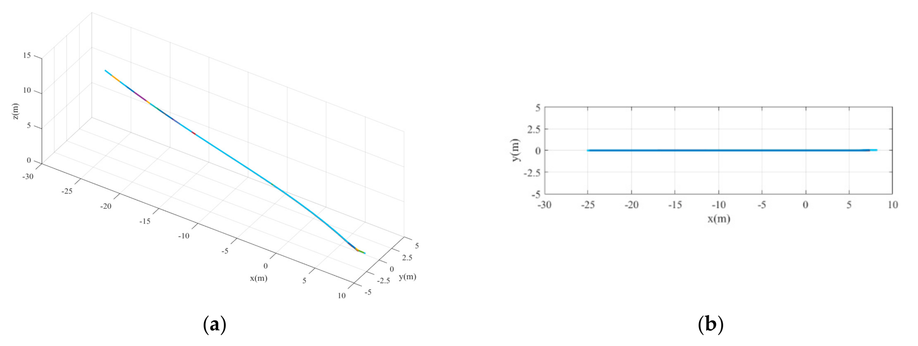
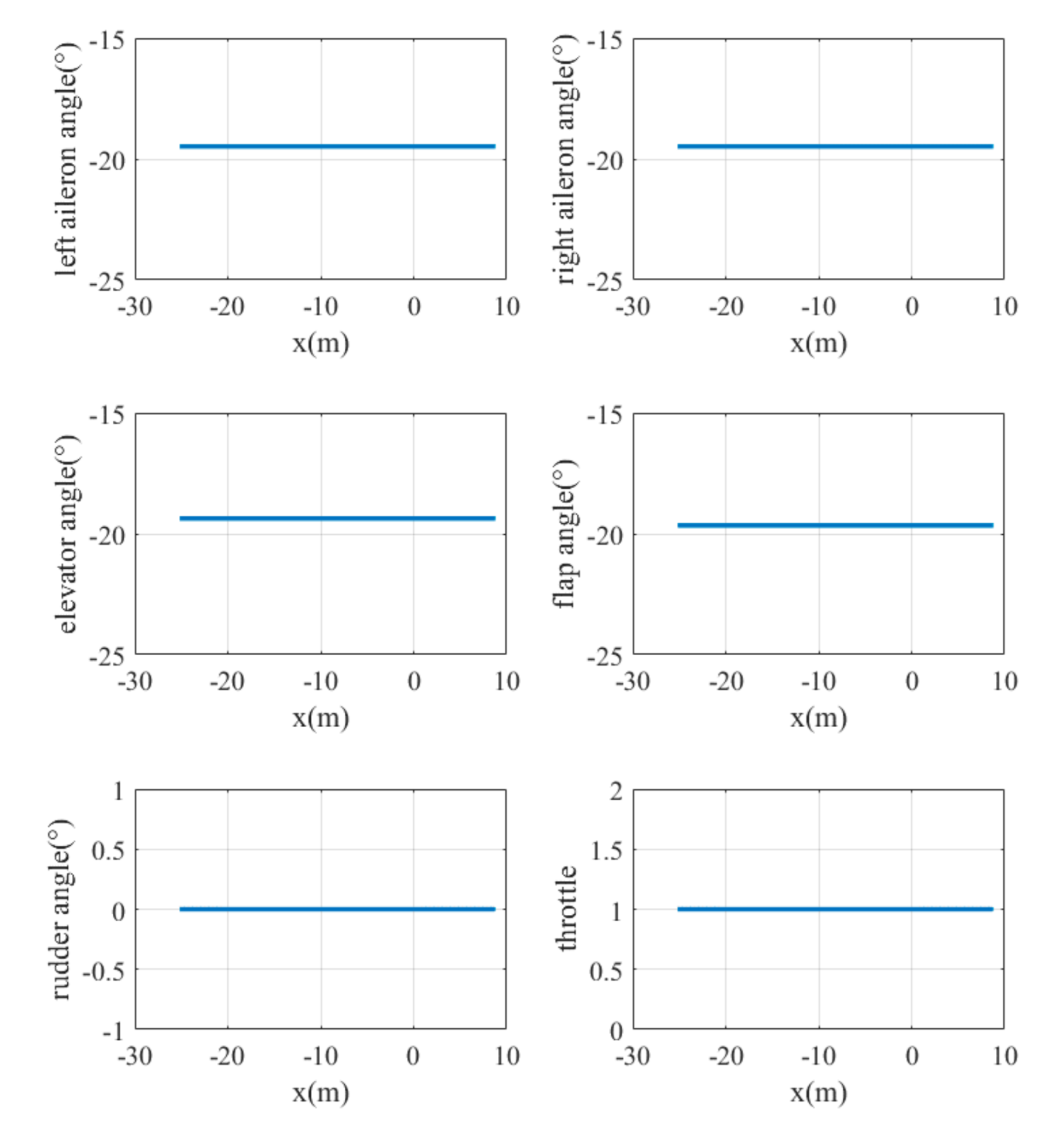
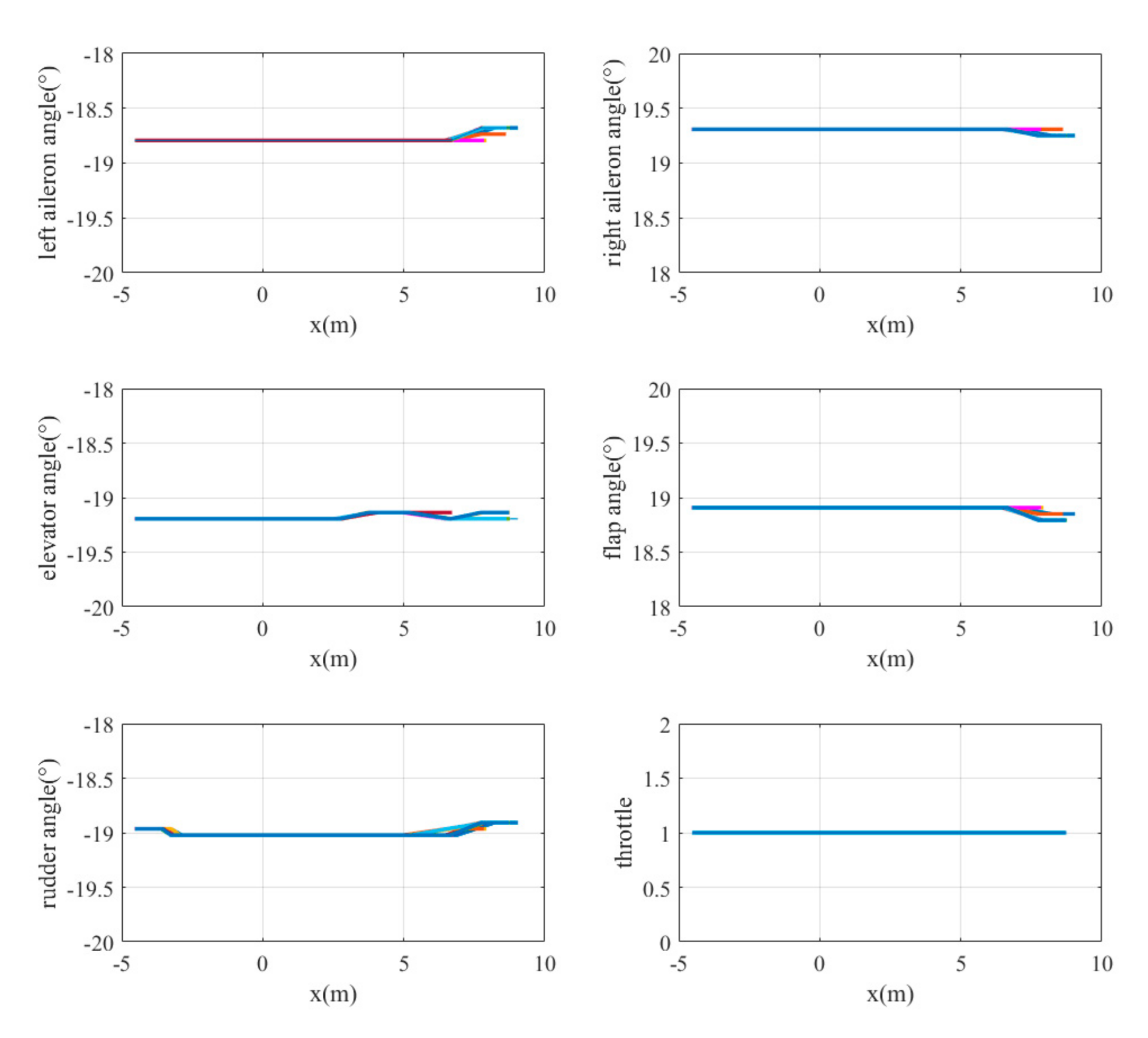
The landing trajectories of the mass point of the UAV model are shown in Figure 10. The final height is less than 0.17 m and the lateral error is less than 0.04 m. The curves of UAV states, including its global linear velocities () and angular velocities with respect to the body frame () varying with position, are shown in Figure 11. The y-axis velocity of the UAV is maintained at around 0 m/s, and the angular velocity of the x-axis vibrates at around −0.15 rad/s before touching the ground. It is obvious that the states of UAV change dramatically during the last seconds. The main reason for this is the lack of landing gear, meaning that part of the body always lands first, leading to irregular motion close to the ground. And this phenomenon also occurs in other conditions. The control commands of the six actuators varying with position are also shown in Figure 12. It can be seen that the rudder exhibits little change from zero, which matches the fact that there is no need for the UAV to steer its yaw angle when it starts landing from the point that exactly aligned with the centerline of the runway.
5.3.2. Case 2
For the second case, the initial position of the UAV is (−25, −2, 12) m. The initial deflection angle of the left and right ailerons, the elevator, and the flaps of the UAV is −0.35 rad. In addition, that of the rudder is 0 rad. The initial velocity along the x-axis is about 10 m/s. There is no disturbance outside. As in case 1, the border of the x-axis is [−30, 50] m and that for the y-axis is [−10, 10] m. Screenshots taken during the landing and the corresponding processed images are shown in Figure 13.
The landing trajectories are shown in Figure 14. It is obvious that the UAV is not aligned with the center line of the runway at the beginning. However, it can adjust itself to land on the centerline of the runway. The final height is below 0.18 m and the final lateral error is less than 0.5 m. The curves of the UAV states, including its linear velocities with reference to the world frame () and body rates () varying with position are shown in Figure 15. The velocities along the x-axis and the y-axis first increase and then decrease. Both the pitch rate and the yaw rate vibrate a little. The control commands of the six actuators varying with position are also shown in Figure 16. The sign of the left and the right aileron are opposite. In addition, the rudder provides a small negative deflection that steers the UAV towards the center of the runway to eliminate the initial lateral offset.
5.3.3. Case 3
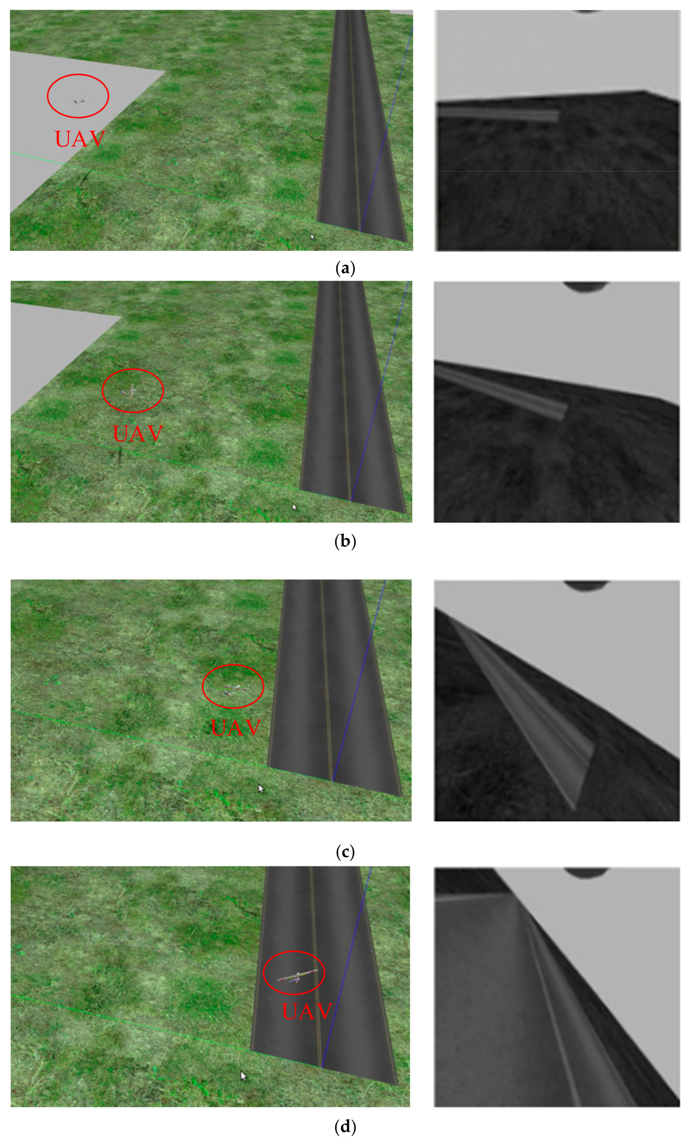
For the third case, the initial position of the UAV is (−4.5, 28, 12) m. The initial deflection angle of the left and right ailerons, the elevator, and the flaps is −0.35 rad. In addition, that of the rudder is 0 rad. The initial velocity along the y-axis is −10 m/s. There is no disturbance outside. The border of the x-axis is [−10, 50] m and for the y-axis is [−30, 30] m. Screenshots taken during the landing and the corresponding processed images are shown in Figure 17.
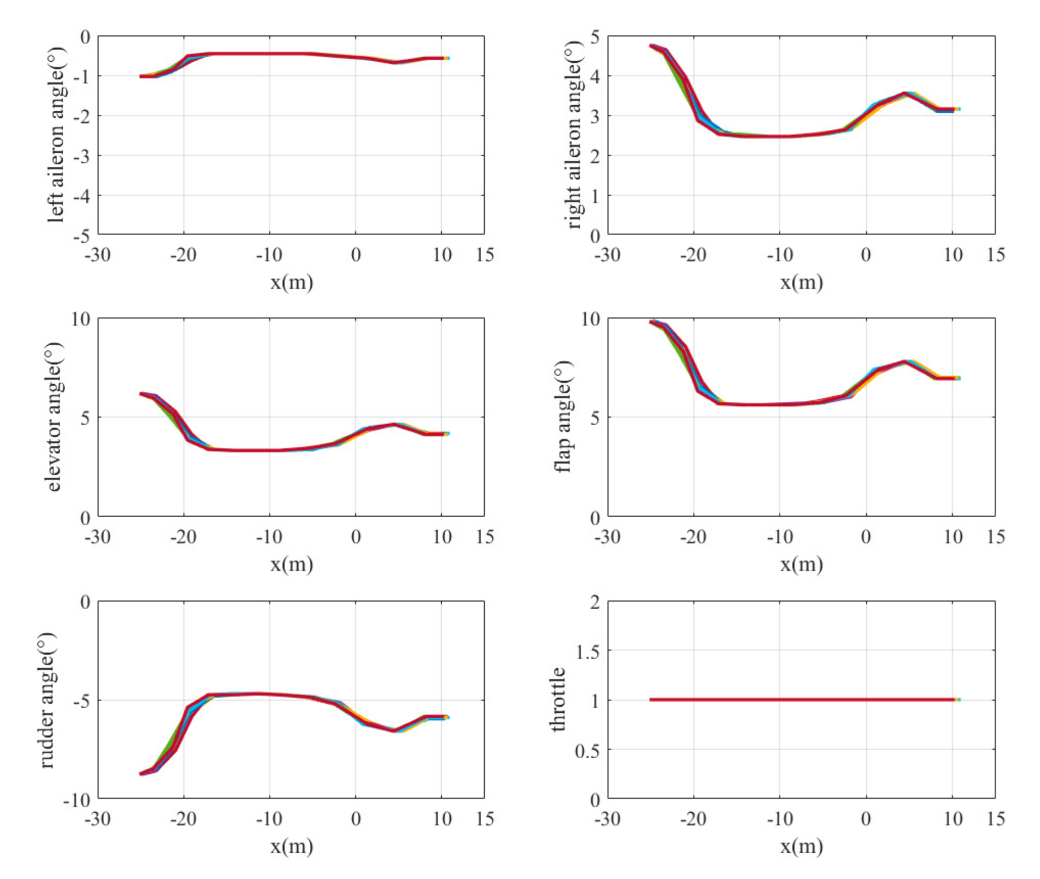
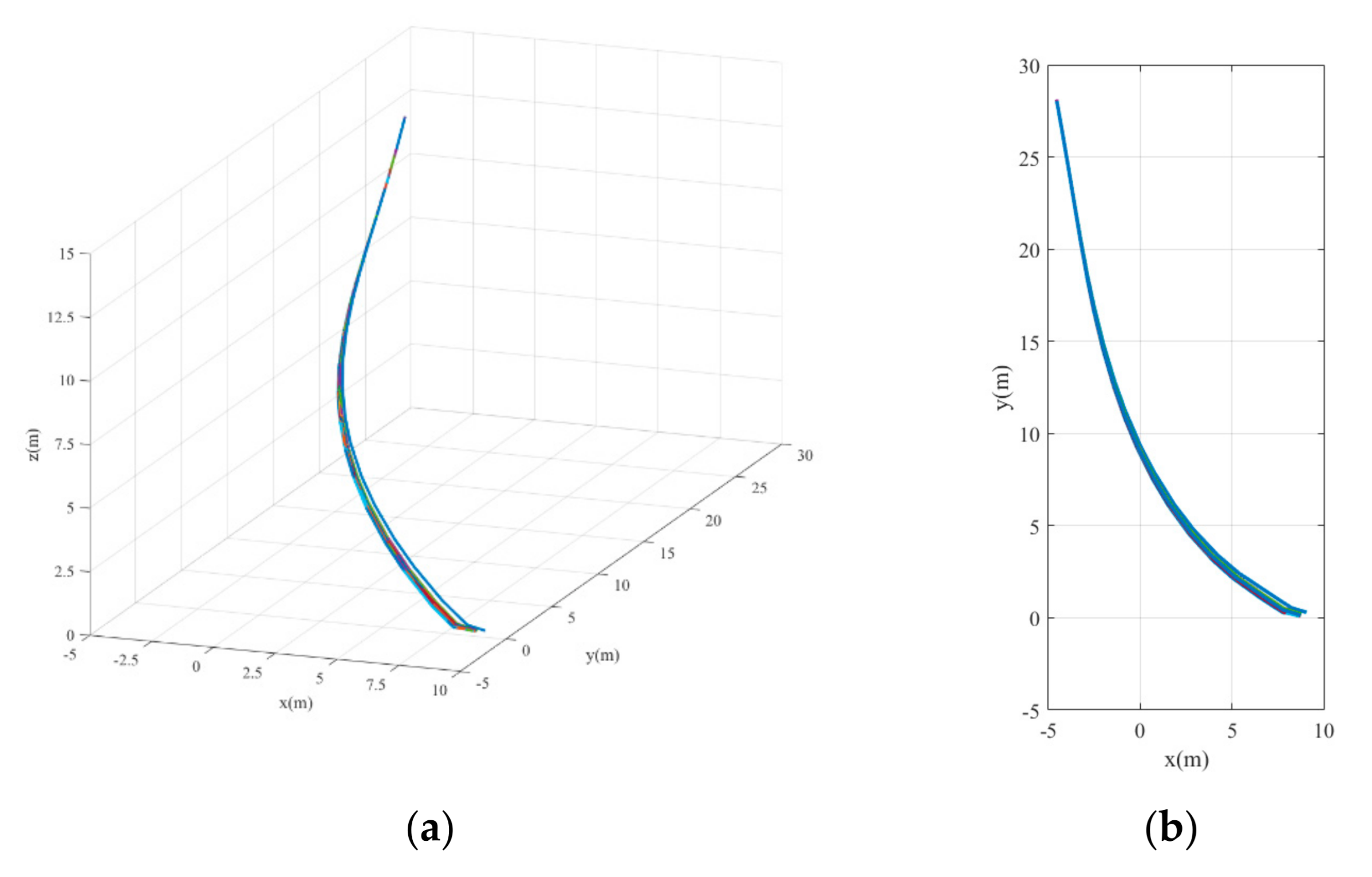
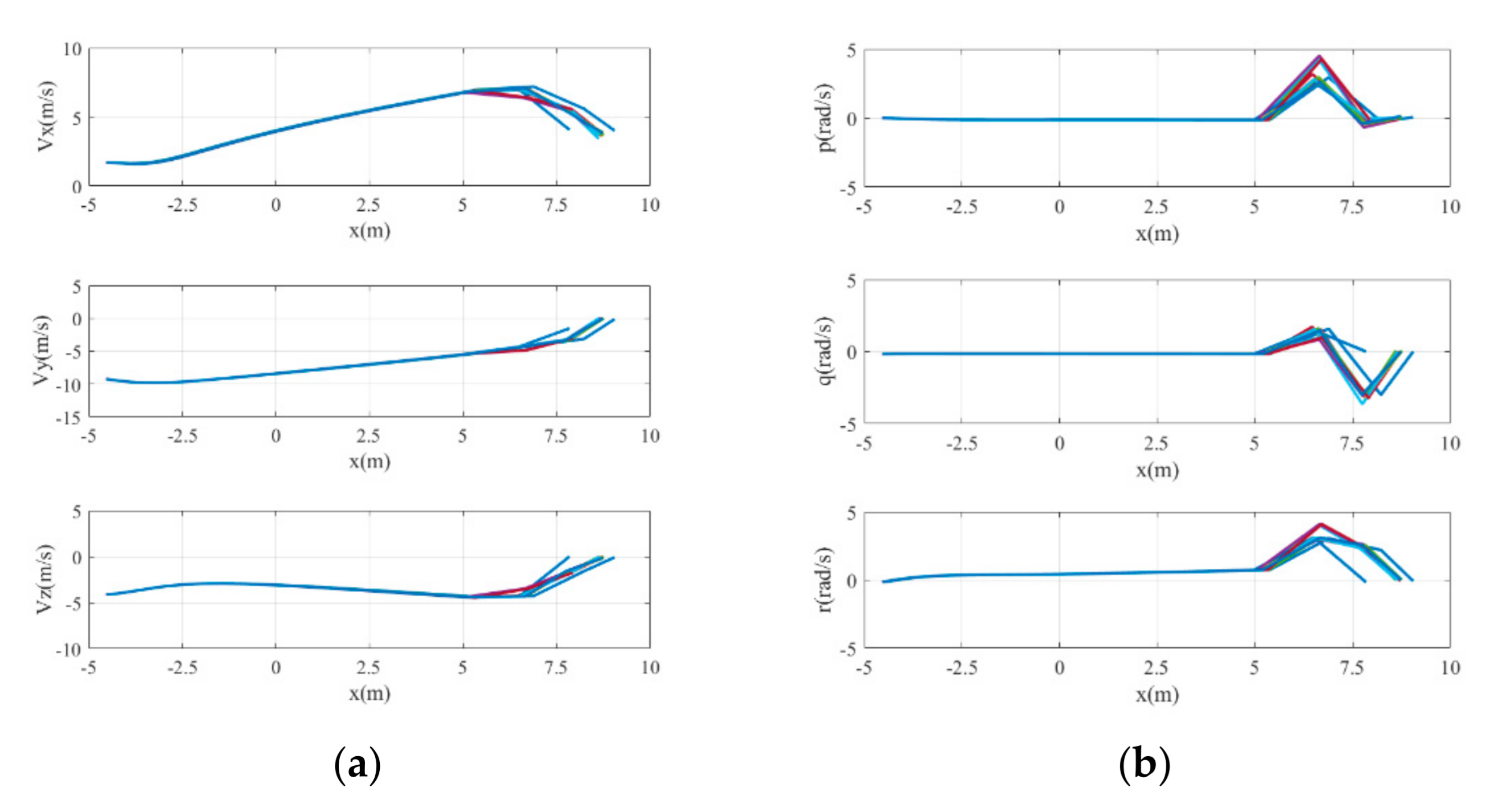
The landing trajectories are shown in Figure 18. They indicate that the UAV makes a turn under this condition and that the distance between the UAV and the centerline of the runway shrinks during its landing. The final height is less than 0.17 m and the lateral error is less than 0.3 m. The curves of UAV states including its global linear velocities () and body rates () varying with position are shown in Figure 19. The velocity of the x-axis first increases and then decreases. The velocity of the y-axis continuously decreases and the yaw rate increases during the adjustment of the heading direction of the UAV. The control commands of the six actuators varying with position are also shown in Figure 20. The rudder has a large negative deflection angle to generate the yaw moment.
5.4. Discussion
The simulation results under different cases confirm that the proposed end-to-end deep reinforcement learning-based method is able to generate appropriate actuator control commands directly on the basis of the input image in order to perform landing in a fixed-wing UAV. After training, the UAV was able to handle the control pattern of landing from different initial points with a final height error within 0.2 m and a lateral error within 0.5 m. Case 1 was the basic situation, with zero lateral offset and zero heading angle offset. Case 2 proved that the UAV was able to learn to eliminate the initial lateral offset. In Case 3, although the UAV started with a large heading angle offset of nearly and a relatively large distance away from the centerline of the runway of nearly 30 m, it was still able to gradually adjust its direction and land successfully. It is worth noting that the quantitative results reflect the general variation tendency of the UAV states during the landing process except for the last phases. The drastic fluctuation of the UAV states when the craft is close to the ground mainly results from the simulated aircraft model. The lack of landing gear means that part of the body always lands first, leading to irregular motion close to the ground. Additionally, the constraints to the final attitudes of the UAV maybe not strict enough.
6. Conclusions
An end-to-end autonomous control method based on DRL is proposed in this paper and validated on the basis of several simulation experiments under the example case of fixed-wing UAV landing. By virtue of the powerful feature representation ability of the deep neural network, the input image can be directly interpreted to generate continuous actuator control commands. In addition, the model-free reinforcement learning algorithm allows the agent to learn the control policy without prior information about the dynamics. We believe that the idea of end-to-end control can be applied in other missions, and that it has the potential to simplify the deployment of cascade controllers in flight experiments with proper adjustment.
For future work, other neural network architectures and learning algorithms will be explored in order to improve the performance. Then, flight experiments will be conducted regarding the training results in the simulation, deploying part of or the whole end-to-end network in the autonomous control of a UAV in a specific scenario. In addition, a further comparison between the proposed method with the traditional method will be performed. Additionally, we expect that the proposed end-to-end autonomous control method can be used in a variety of missions other than landing, in which the constraints need to be considered with respect to practical problems and the reward function and terminal state criterion should be reasonably determined.
Author Contributions
Conceptualization, J.Z. and Z.C.; Methodology, J.Z., J.S. and L.W.; Project administration, J.Z.; Resources, Z.C. and Y.W.; Writing—original draft, J.Z. and J.S.; Writing—review & editing, J.S. All authors have read and agreed to the published version of the manuscript.
Funding
This research was funded by the Aeronautical Science Foundation of China (No. 20175851032) and Fundamental Research Funds for the Central Universities of China (No.YWF-21-BJ-J-541).
Institutional Review Board Statement
Not applicable.
Informed Consent Statement
Not applicable.
Data Availability Statement
No new data were created or analyzed in this study. Data sharing is not applicable to this article.
Conflicts of Interest
The authors declare no conflict of interest.
References
- Zhen, Z.; Zhu, P.; Xue, Y.; Ji, Y. Distributed intelligent self-organized mission planning of multi-UAV for dynamic targets cooperative search-attack. Chin. J. Aeronaut. 2019, 32, 2706–2716. [Google Scholar] [CrossRef]
- Li, S.; Liu, T.; Zhang, C. Learning unmanned aerial vehicle control for autonomous target following. arXiv 2017, arXiv:1709.08233. [Google Scholar]
- Wang, C.; Wu, L.; Yan, C.; Wang, Z.; Long, H.; Yu, C. Coactive design of explainable agent-based task planning and deep reinforcement learning for human-UAVs teamwork. Chin. J. Aeronaut. 2020, 33, 2930–2945. [Google Scholar] [CrossRef]
- Tang, S.; Kumar, V. Autonomous flight. Annu. Rev. Control Robot. Auton. Syst. 2018, 1, 29–52. [Google Scholar] [CrossRef]
- Lu, Y.; Xue, Z.; Xia, G.-S.; Zhang, L. A survey on vision-based UAV navigation. Geo Spat. Inf. Sci. 2018, 21, 21–32. [Google Scholar] [CrossRef] [Green Version]
- Gasparetto, A.; Boscariol, P.; Lanzutti, A.; Vidoni, R. Path planning and trajectory planning algorithms: A general overview. Motion Oper. Plan. Robot. Syst. 2015, 29, 3–27. [Google Scholar] [CrossRef]
- Yang, T.; Li, P.; Zhang, H.; Li, J.; Li, Z. Monocular vision SLAM-based UAV autonomous landing in emergencies and unknown environments. Electronics 2018, 7, 73. [Google Scholar] [CrossRef] [Green Version]
- Chen, J.; Liu, T.; Shen, S. Online generation of collision-free trajectories for quadrotor flight in unknown cluttered environments. In Proceedings of the 2016 IEEE International Conference on Robotics and Automation (ICRA), Stockholm, Sweden, 16–21 May 2016; IEEE Press: Piscataway, NJ, USA, 2016; pp. 1476–1483. [Google Scholar]
- Bagnell, J.A.; Bradley, D.; Silver, D.; Silver, D.; Sofman, B.; Stentz, A. Learning for autonomous navigation. IEEE Robot. Autom. 2010, 17, 7–84. [Google Scholar] [CrossRef]
- Mnih, V.; Kavukcuoglu, K.; Silver, D. Playing atari with deep reinforcement learning. arXiv 2013, arXiv:1312.5602. [Google Scholar]
- Chrittwieser, J.; Antonoglou, I.; Hubert, T.; Simonyan, K.; Sifre, L.; Schmitt, S.; Guez, A.; Lockhart, E.; Hassabis, D.; Graepel, T.; et al. Mastering atari, go, chess and shogi by planning with a learned model. Nature 2020, 588, 604–609. [Google Scholar] [CrossRef]
- Li, X.; Chen, Y.; Li, L. End-to-end task-completion neural dialogue systems. arXiv 2017, arXiv:1703.01008. [Google Scholar]
- Bahdanau, D.; Brakel, P.; Xu, K.; Goyal, A.; Lowe, R.; Pineau, J.; Courville, A.; Bengio, Y. An actor-critic algorithm for sequence prediction. arXiv 2016, arXiv:1607.07086. [Google Scholar]
- Kiran, B.R.; Sobh, I.; Talpaert, V.; Mannion, P.; Al Sallab, A.A.; Yogamani, S.; Perez, P. Deep reinforcement learning for autonomous driving: A survey. IEEE Trans. Intell. Transp. Syst. 2021, 1–18. [Google Scholar] [CrossRef]
- Guo, T.; Jiang, N.; Li, B.; Zhu, X.; Wang, Y.; Du, W. UAV navigation in high dynamic environments: A deep reinforcement learning approach. Chin. J. Aeronaut. 2020, 34, 479–489. [Google Scholar] [CrossRef]
- Levine, S.; Finn, C.; Darrell, T.; Abbeel, P. End-to-end training of deep visuomotor policies. J. Mach. Learn. Res. 2016, 17, 1334–1373. [Google Scholar]
- Lee, J.; Hwangbo, J.; Wellhausen, L.; Koltun, V.; Hutter, M. Learning quadrupedal locomotion over challenging terrain. Sci. Robot. 2020, 5, eabc5986. [Google Scholar] [CrossRef]
- Xiong, G.; Dong, L. Vision-based autonomous tracking of UAVs based on reinforcement learning. In Proceedings of the 2020 Chinese Automation Congress (CAC), Shanghai, China, 6–8 November2020; IEEE Press: Piscataway, NJ, USA, 2020; pp. 2682–2686. [Google Scholar]
- Sampedro, C.; Rodriguez-Ramos, A.; Gil, I. Image-based visual servoing controller for multirotor aerial robots using deep reinforcement learning. In Proceedings of the 2018 IEEE/RSJ International Conference on Intelligent Robots and Systems (IROS), Madrid, Spain, 1–5 October 2018; IEEE Press: Piscataway, NJ, USA, 2018; pp. 979–986. [Google Scholar]
- Mercado-Ravell, D.A.; Castillo, P.; Lozano, R. Visual detection and tracking with UAVs, following a mobile object. Adv. Robot. 2019, 33, 388–402. [Google Scholar] [CrossRef]
- Kumar, K.S.; Venkatesan, M.; Karuppaswamy, S. Lidar-aided autonomous landing and vision-based taxiing for fixed-wing UAV. J. Indian Soc. Remote. Sens. 2021, 49, 629–640. [Google Scholar] [CrossRef]
- Falanga, D.; Zanchettin, A.; Simovic, A.; Delmerico, J.; Scaramuzza, D. Vision-based autonomous quadrotor landing on a moving platform. In Proceedings of the 2017 IEEE International Symposium on Safety, Security and Rescue Robotics (SSRR), Shanghai, China, 11–13 October 2017; IEEE Press: Piscataway, NJ, USA, 2017; pp. 200–207. [Google Scholar]
- Asl, H.J.; Yoon, J. Robust image-based control of the quadrotor unmanned aerial vehicle. Nonlinear Dyn. 2016, 85, 2035–2048. [Google Scholar]
- Shuai, C.; Wang, H.; Zhang, W.; Yao, P.; Qin, Y. Binocular vision perception and obstacle avoidance of visual simulation system for power lines inspection with UAV. In Proceedings of the 2017 36th Chinese Control Conference (CCC), Dalian, China, 26–28 July 2017; IEEE Press: Piscataway, NJ, USA, 2017; pp. 10480–10485. [Google Scholar]
- Mohta, K.; Kumar, V.; Daniilidis, K. Vision-based control of a quadrotor for perching on lines. In Proceedings of the 2014 IEEE International Conference on Robotics and Automation (ICRA), Hong Kong, China, 31 May–7 June 2014; IEEE Press: Piscataway, NJ, USA, 2014; pp. 3130–3136. [Google Scholar]
- Falanga, D.; Mueggler, E.; Faessler, M.; Scaramuzza, D. Aggressive quadrotor flight through narrow gaps with onboard sensing and computing using active vision. In Proceedings of the 2017 IEEE international conference on robotics and automation (ICRA), Singapore, 2 May–3 June 2017; IEEE Press: Piscataway, NJ, USA, 2017; pp. 5774–5781. [Google Scholar]
- Mohta, K.; Watterson, M.; Mulgaonkar, Y.; Liu, S.; Qu, C.; Makineni, A.; Saulnier, K.; Sun, K.; Zhu, A.; Delmerico, J.; et al. Fast, autonomous flight in GPS-denied and cluttered environments. J. Field Robot. 2017, 35, 101–120. [Google Scholar] [CrossRef]
- Lin, Y.; Gao, F.; Qin, T.; Gao, W.; Liu, T.; Wu, W.; Yang, Z.; Shen, S. Autonomous aerial navigation using monocular visual-inertial fusion. J. Field Robot. 2017, 35, 23–51. [Google Scholar] [CrossRef]
- Schmid, K.; Lutz, P.; Tomić, T.; Mair, E.; Hirschmüller, H. Autonomous vision-based micro air vehicle for indoor and outdoor navigation. J. Field Robot. 2014, 31, 537–570. [Google Scholar] [CrossRef]
- Basso, M.; de Freitas, E.P. A UAV Guidance system using crop row detection and line follower algorithms. J. Intell. Robot. Syst. 2019, 97, 605–621. [Google Scholar] [CrossRef]
- Ross, S.; Melik-Barkhudarov, N.; Shankar, K.S.; Wendel, A.; Dey, D.; Bagnell, J.A. Learning monocular reactive UAV control in cluttered natural environments. In Proceedings of the 2013 IEEE International Conference on Robotics and Automation, Karlsruhe, Germany, 6–10 May 2013; IEEE Press: Piscataway, NJ, USA, 2013; pp. 1765–1772. [Google Scholar]
- Loquercio, A.; Maqueda, A.I.; del-Blanco, C.R.; Scaramuzza, D. DroNet: Learning to fly by driving. IEEE Robot. Autom. Lett. 2018, 3, 1088–1095. [Google Scholar] [CrossRef]
Figure 1.
Description of a general reinforcement learning problem.

Figure 2.
Comparison of the traditional control and end-to-end control pipelines.

Figure 3.
The image-based RL framework for a UAV control problem.

Figure 4.
The network architectures: (a) the architecture of the actor-network; (b) the architecture of the critic-network.
Figure 4.
The network architectures: (a) the architecture of the actor-network; (b) the architecture of the critic-network.

Figure 5.
The diagram of the algorithm implementation.

Figure 6.
The relationship of the UAV model and the proposed controller.

Figure 7.
The simulation environment and setup.

Figure 8.
The computing graph of the simulation program.

Figure 9.
The landing process under case 1 (a–e). (a) t = 0.0 s; (b) t = 1.08 s; (c) t = 2.10 s; (d) t = 3.07 s; (e) t = 4.12 s.
Figure 9.
The landing process under case 1 (a–e). (a) t = 0.0 s; (b) t = 1.08 s; (c) t = 2.10 s; (d) t = 3.07 s; (e) t = 4.12 s.


Figure 10.
The landing trajectories under case 1. (a) 3D trajectory. (b) 2D trajectory in the x-y plane.
Figure 10.
The landing trajectories under case 1. (a) 3D trajectory. (b) 2D trajectory in the x-y plane.

Figure 11.
The UAV states under case 1. (a) global linear velocities. (b) body rates.

Figure 12.
The control commands for the actuators under case 1.

Figure 13.
The landing process under case 2 (a–e). (a) t = 0.0 s; (b) t = 0.13 s; (c) t = 1.09 s; (d) t = 2.11 s; (e) t = 3.06 s.
Figure 13.
The landing process under case 2 (a–e). (a) t = 0.0 s; (b) t = 0.13 s; (c) t = 1.09 s; (d) t = 2.11 s; (e) t = 3.06 s.


Figure 14.
The landing trajectories under case 2. (a) 3D trajectory. (b) 2D trajectory in the x-y plane.
Figure 14.
The landing trajectories under case 2. (a) 3D trajectory. (b) 2D trajectory in the x-y plane.

Figure 15.
The UAV states under case 2. (a) global linear velocities. (b) body rates.

Figure 16.
The control commands for the actuators under case 2.

Figure 17.
The landing process under case 3 (a–e). (a) t = 0.0 s; (b) t = 0.24 s; (c) t = 2.03 s; (d) t = 2.22 s; (e) t = 3.13 s.
Figure 17.
The landing process under case 3 (a–e). (a) t = 0.0 s; (b) t = 0.24 s; (c) t = 2.03 s; (d) t = 2.22 s; (e) t = 3.13 s.


Figure 18.
The landing trajectories under case 3. (a) 3D trajectory. (b) 2D trajectory in the x-y plane.
Figure 18.
The landing trajectories under case 3. (a) 3D trajectory. (b) 2D trajectory in the x-y plane.

Figure 19.
The UAV states under case 3. (a) global linear velocities. (b) body rates.

Figure 20.
The control commands for the actuator under case 3.


Table 1.
The initial conditions of the three different cases.
| Case 1 | Exactly aligned with the centerline of the runway |
| Case 2 | Parallel to the centerline of the runway with a small lateral offset |
| Case 3 | Vertical to the runway with a large lateral offset |
Publisher’s Note: MDPI stays neutral with regard to jurisdictional claims in published maps and institutional affiliations. |
© 2021 by the authors. Licensee MDPI, Basel, Switzerland. This article is an open access article distributed under the terms and conditions of the Creative Commons Attribution (CC BY) license (https://creativecommons.org/licenses/by/4.0/).
Share and Cite
MDPI and ACS Style
Zhao, J.; Sun, J.; Cai, Z.; Wang, L.; Wang, Y. End-to-End Deep Reinforcement Learning for Image-Based UAV Autonomous Control. Appl. Sci. 2021, 11, 8419. https://0-doi-org.brum.beds.ac.uk/10.3390/app11188419
AMA Style
Zhao J, Sun J, Cai Z, Wang L, Wang Y. End-to-End Deep Reinforcement Learning for Image-Based UAV Autonomous Control. Applied Sciences. 2021; 11(18):8419. https://0-doi-org.brum.beds.ac.uk/10.3390/app11188419
Chicago/Turabian StyleZhao, Jiang, Jiaming Sun, Zhihao Cai, Longhong Wang, and Yingxun Wang. 2021. "End-to-End Deep Reinforcement Learning for Image-Based UAV Autonomous Control" Applied Sciences 11, no. 18: 8419. https://0-doi-org.brum.beds.ac.uk/10.3390/app11188419
Note that from the first issue of 2016, this journal uses article numbers instead of page numbers. See further details here.