Scheduling Period Selection Based on Stability Analysis for Engagement Control Task of Automatic Clutches

Abstract

The clutch engagement process involves three phases known as open, slipping, and locked and takes a few seconds. The engagement control program runs in an embedded control unit, in which discretization may induce oscillation and even instability in the powertrain due to an improper scheduling period for the engagement control task. To properly select the scheduling period, a methodology for control–scheduling co-design during clutch engagement is proposed. Considering the transition of the friction state from slipping to being locked, the co-design framework consists of two steps. In the first step, a stability analysis is conducted for the slipping phase based on a linearized system model enveloping the driving and driven part of the clutch, feed-forward and feedback control loop together with a zero-order signal hold element. The critical period is determined according to pole locations, and factors influencing the critical period are investigated. In the second step, real-time hardware-in-the-loop experiments are carried out to inspect the dynamic response concerning the friction state transition. A sub-boundary within the stable region is found to guarantee the control performance to satisfy the engineering requirements. In general, the vehicle jerk and clutch frictional loss increase with the increase in the scheduling period. When the scheduling period is shorter than the critical period, the rate of increase is mild. However, once the scheduling period exceeds the critical period, the rate of increase becomes very high.

1. Introduction

Automatic clutches are key enablers for various automatic transmissions in vehicles, such as automated manual transmissions, hydraulic automatic transmissions, and electric variable transmissions [1,2,3]. Due to the piecewise nonlinearity of the friction torque generated on the clutch plates, the clutch engagement control has to handle the three phases from open to slipping, and then to locked [4,5]. As required by the dynamic performance of vehicles, the engagement process should be completed in as short a period as possible [6,7]. In real application, the control program for clutch engagement runs in an embedded control unit together with other programs related to the control of automatic transmissions. Hence, multiple programs are implemented in the discrete time domain and share the computational resources of the control unit, which is coordinated by the task scheduler. In recent years, complex programs have been developed with the aim of improving adaptability [8,9] and robustness [10,11]; consequently, the computational load increases, and the negative effects of the discretization emerge. As shown in the literature [12,13,14], discretization results in different dynamic behavior and is one of the reasons for the instability of digital control systems. Therefore, the task scheduling period should be selected carefully considering both the control performance and the limitations of the computational resources. Thus far, the control–scheduling co-design for clutch engagement has not been studied, even though it is urgently needed for the rapid development of the transmission industry.

The control–scheduling co-design for real-time applications can be classified into two types in regard to the modeling method of the control system. The first type considers the control system as a set of periodic real-time tasks represented by time parameters, in which the optimal design is used to select the scheduling periods by considering the limits on the computational resources. For example, delay and jitter were regarded as the characteristics of the tasks, and global optimization was performed according to simulated annealing in [15]. In [16], each real-time task was divided into a mandatory part and an optional part, and optimal reward-based scheduling was applied to the tasks. In [17], branch and bound-based techniques were proposed for determining optimal schedules under different restrictions on the adaptability of execution rates for the tasks. However, the performance of the system is considered to be directly proportional to the time taken to stabilize all functionalities. Obviously, the dynamic performance of the control system cannot be explicitly reflected.

With the aim of overcoming this deficiency, the second type of control–scheduling co-design employs state equations to describe the control system. The performance is measured by using the control plant information, such as plant states [18], control inputs [19], and a cost function for the states and inputs [20]. Various schedulers have been designed to guarantee the system stability. For example, a feedback scheduler that periodically assigns new sampling periods was developed based on estimates of the current plant states and noise intensities for a linear stochastic system [20]. The proof of the schedulability condition also serves as a systematic method to design a scheduler for a networked linear time-invariant system [19]. By designing an exponential stable fault detector, a real-time feedback scheduler was developed for a linear discrete system, considering time delay and data dropouts of the network transmission [21]. An integrated design for a hybrid scheduling strategy, an adaptive quantizer and a feedback controller for a linear networked control system was developed to maintain asymptotic stability by using the multiple-Lyapunov function and switched system theory [18]. The co-design of control law, bandwidth scheduling and event generator to guarantee globally uniformly asymptotic stability was formulated as a linear matric inequality problem [22]. The sufficient stability condition was derived for each plant by the simultaneous stabilization of a collection of plants remotely controlled via a wireless network [23]. Nevertheless, no previous literature has provided the effect of the scheduling period on the critical boundary with regard to stability and on the control performance once the stability condition is satisfied. Besides, most of the studies in the literature refer to linear systems. Their methods and conclusions cannot be directly applied to the piecewise nonlinear system used as the powertrain during clutch engagement.

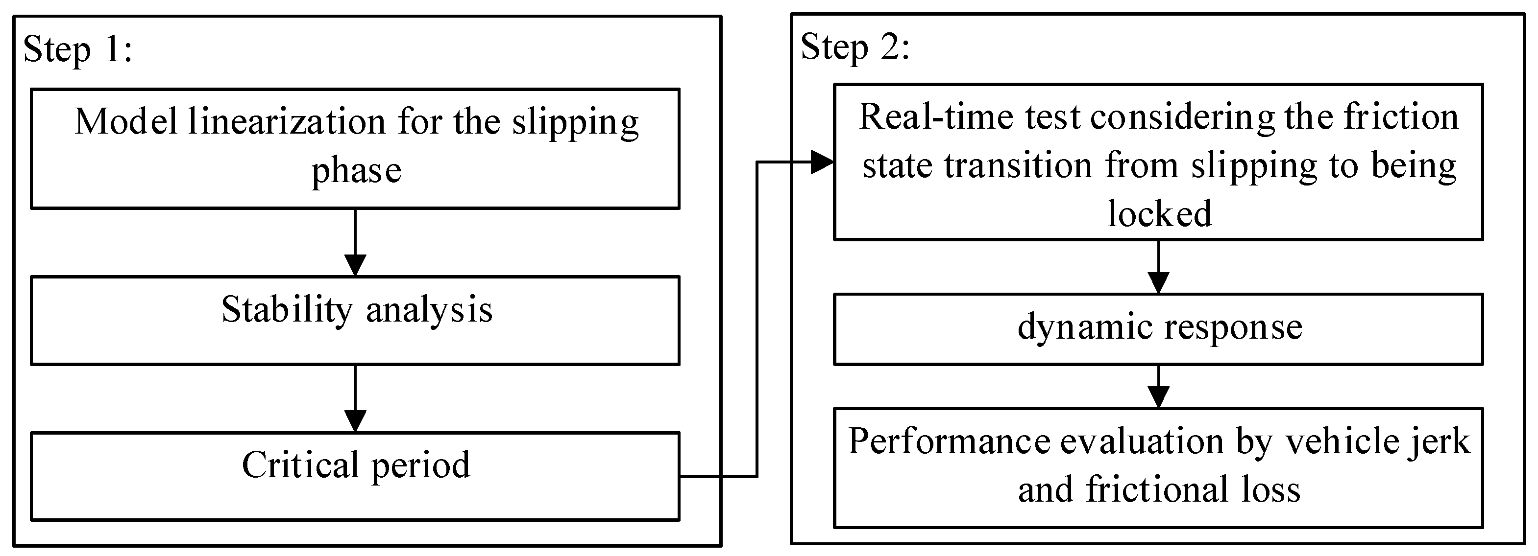
In this study, a two-step control–scheduling co-design framework is proposed for clutch engagement, as depicted in Figure 1. Since each segment is linear in a piecewise nonlinear system, the powertrain model can be regarded as linear when the clutch is slipping. Thus, in the first step, the stability analysis can be conducted according to the pole locations of the integrated system model that envelops the clutch-employed powertrain model, the feedback control law and the zero-order holder. In this way, the critical period regarding stability can be determined, and factors influencing the critical period can be investigated. In the second step, the transition between adjacent segments, from the slipping to the being locked phase of the clutch-employed powertrain dynamics is investigated. The dynamic performance is evaluated in terms of vehicle jerk and frictional loss during clutch engagement. The dynamic responses are obtained by real-time hardware-in-the-loop experiments and the performances of different scheduling periods within the stable region can be compared.

The major contributions of this paper are summarized as:

(1) A two-step framework of control–scheduling co-design for selecting the task scheduling period is proposed for clutch engagement control.

(2) The sensitivity analysis of the critical period with regard to stability based on five key parameters—the natural frequency, damping coefficient, proportional gain, integral gain, and time delay—is illustrated.

(3) The effect of scheduling period on dynamic performance during clutch engagement is exposed by real-time hardware-in-the-loop experiments. A sub-boundary of the scheduling period within the stable region is found to guarantee the control performance.

This paper is organized as follows. The system model under closed-loop control is described in Section 2. In Section 3, the model is linearized and discretized for the slipping phase, and the stability condition is derived according to pole locations. Thereafter, a sensitivity analysis is conducted. In Section 4, the system runs on a hardware-in-the-loop platform, and the dynamic responses are obtained to evaluate clutch engagement performance. Finally, conclusions are drawn in Section 5.

2. System Modeling

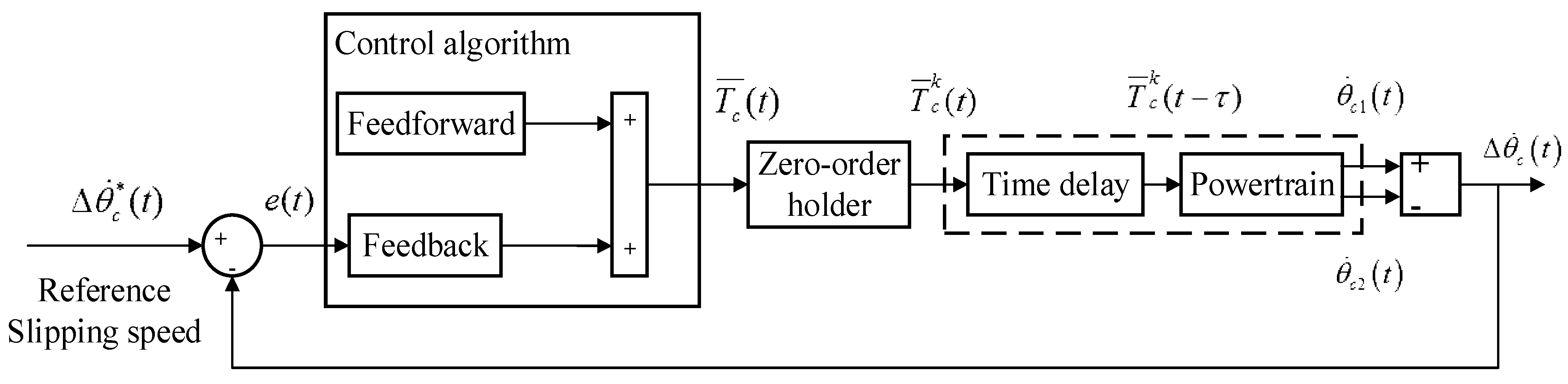
The diagram of a closed-loop control system during clutch engagement is depicted in Figure 2. The system consists of a powertrain with actuation delay, a control algorithm, and a zero-order holder. The model for each subsystem is described in the following paragraphs.

2.1. Powertrain Model

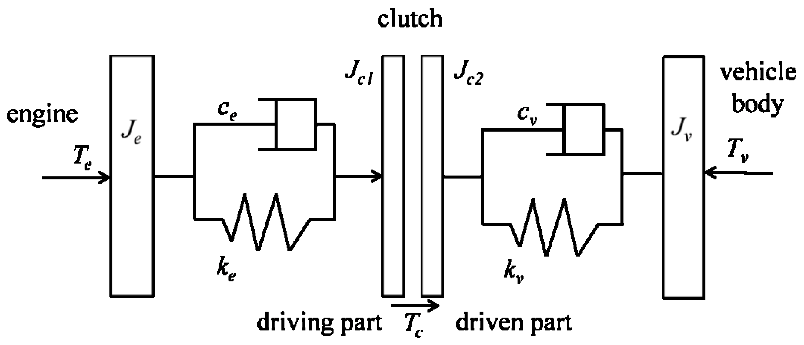
The lumped dynamic model of the powertrain is depicted in Figure 3. The model consists of the engine, the clutch (with separate driving and driven parts), the vehicle body, the elastic connection between the engine and the clutch, and the elastic connection between the clutch and the vehicle body.

The model has four degrees of freedom. The governing equations are presented below. Equations (1) and (2) represent the dynamics of the engine-side components separated by the clutch. Similarly, Equations (3) and (4) represent the dynamics of the body-side components. The time delay $\tau$ is used to describe the inevitable delay of the actuators due to a variety of factors, such as the electromotive force of the motor-driven system and the filling process of the hydraulic system.

$$J_e{\ddot{\theta }}_e\left(t\right)=T_e\left(t\right)-c_e\left({\dot{\theta }}_e\left(t\right)-{\dot{\theta }}_{c1}\left(t\right)\right)e-k_e\left({\theta }_e\left(t\right)-{\theta }_{c1}\left(t\right)\right)$$

(1)

$$J_{c1}{\ddot{\theta }}_{c1}\left(t\right)=c_e\left({\dot{\theta }}_e\left(t\right)-{\dot{\theta }}_{c1}\left(t\right)\right)+k_e\left({\theta }_e\left(t\right)-{\theta }_{c1}\left(t\right)\right)-T_c\left(t-\tau \right)$$

(2)

$$J_{c2}{\ddot{\theta }}_{c2}\left(t\right)=T_c\left(t-\tau \right)-c_v\left({\dot{\theta }}_{c2}\left(t\right)-{\dot{\theta }}_v\left(t\right)\right)-k_v({\theta }_{c2}\left(t\right)-{\theta }_v\left(t\right))$$

(3)

$$J_v{\ddot{\theta }}_v\left(t\right)=c_v\left({\dot{\theta }}_{c2}\left(t\right)-{\dot{\theta }}_v\left(t\right)\right)+k_v\left({\theta }_{c2}\left(t\right)-{\theta }_v\left(t\right)\right)-T_v\left(t\right)$$

(4)

The clutch transmitted torque $T_c$ is generated by the friction force between the two friction plates of the clutch. According to the Coulomb law of friction [24], $T_c$ can be described with a piecewise function in terms of the status of the clutch, as follows.

$$T_c\left(t\right)=\{\begin{array}{l}0\mathrm{open}\\ \overline{T_c}\left(t\right)\cdot \mathrm{sign}\left(\Delta {\dot{\theta }}_c\left(t\right)\right)\mathrm{slipping}\\ x\mathrm{in}[\begin{array}{cc}-\overline{T_{cs}}\left(t\right)& \overline{T_{cs}}\left(t\right)\end{array}]\mathrm{locked}\end{array}$$

(5)

where ${\overline{T}}_c$ is the magnitude of the clutch transmitted torque in the slipping phase, and $\overline{T_{cs}}$ is the magnitude limitation of the clutch static friction torque in the locked phase. So, the magnitude of the clutch transmitted torque $T_c$ can be controlled by a clutch actuator in the slipping phase, but it can be any value within $\left[\begin{array}{cc}-{\overline{T}}_{cs}& {\overline{T}}_{cs}\end{array}\right]$ in the locked stage.

In the slipping stage, the magnitude of the clutch torque $T_c$ is proportional to the magnitude of the normal force $F_n$, and the direction of $T_c$ is determined by the slipping speed $\Delta {\dot{\theta }}_c$. Therefore, ${\overline{T}}_c$ can be calculated as follows.

$$\overline{T_c}\left(t\right)=\mu \cdot F_n\left(t\right)\cdot R_c\cdot N$$

(6)

$R_c$ is the effective radius of clutch plate, N is the number of friction surfaces.

The definition of $\Delta {\dot{\theta }}_c$ is given as follows.

$$\Delta {\dot{\theta }}_c\left(t\right)={\dot{\theta }}_{c1}\left(t\right)-{\dot{\theta }}_{c2}\left(t\right)$$

(7)

As indicated by (5), the clutch transmitted torque $T_c$ can be actively controlled only in the slipping stage by applying a proper normal force $F_n$, while the other two stages cannot be controlled by the normal force $F_n$. That is, the clutch torque $T_c$ is zero in the open stage and can be any value within the range defined by the normal force $F_n$ due to the static friction in the locked stage. Therefore, the clutch transmitted torque $T_c$ has a direct effect on the powertrain dynamics, but it has piecewise characteristics.

Referring to the literature on powertrain dynamics and control [25,26], the vehicle load $T_v$ can be calculated as follows:

$$T_v=(F_{air}+F_g+F_r)\cdot R$$

(8)

where

$$F_{air}=0.5\cdot c_D\cdot A_V\cdot {\rho }_{air}\cdot {({\nu }_{air}+v)}^2$$

(9)

$$F_g=m\cdot g\cdot \sin \alpha$$

(10)

$$F_r=m\cdot g\cdot \cos \alpha \cdot f$$

(11)

$$v=i_g\cdot {\dot{\theta }}_v$$

(12)

f is the rolling resistance coefficient.

2.2. Control Algorithm

Considering that the magnitude of the clutch transmitted torque $\overline{T_c}(t)$ can be physically controlled, it is defined as the control input, as shown in Figure 2. Advanced controllers for clutch engagement comprise feed-forward and feedback blocks. Most of the feedback blocks have a PID-like form, and the gains are calculated by the advanced controllers [27,28]. Without loss of generality, a control algorithm consisting of a feed-forward block and a PI feedback loop was modeled in this study. The engine output torque $T_e$, which can be obtained from the engine control unit, is regarded as the feed-forward part of the control input. The deviation from the reference slipping speed of the clutch is considered as the feedback signal. The control algorithm is mathematically expressed as

$$\overline{T_c}(t)=T_e(t)+k_{p}e(t)+k_i{\displaystyle \int e(t)}$$

(13)

where

$$e(t)=\Delta {\dot{\theta }}_c(t)-\Delta {\dot{\theta }}_c^{*}(t)$$

(14)

2.3. Zero-Order Holder

The zero-order holder maintains the value of $\overline{T_c}(t)$ between the time $kT$ and $(k+1)T$. The mathematical expression is as follows.

$${\overline{T}}_c^k(t)={\overline{T}}_c(kT) \left(k=0,1,\cdots ,n\right)\hspace{0.17em}for kT\le t\le (k+1)T$$

(15)

3. Stability Analysis for the Slipping Phase

The first step of the control–scheduling co-design is to conduct a stability analysis for the slipping phase. In this phase, the magnitude of the clutch transmitted torque $T_c$ can be actively controlled because it is generally proportional to the normal force acting on the friction interface. Further, considering that there exists $\mathrm{sign}(\Delta {\dot{\theta }}_c)=1$ (i.e., $\Delta {\dot{\theta }}_c>0$) during clutch engagement, in most cases, especially when the system is stable, the piecewise nonlinearity of the clutch torque $T_c\left(t\right)$, as in (7) can be linearized as $T_c\left(t\right)={\overline{T}}_c\left(t\right)$. Thereafter, the linearization allows the application of stability theory for linear systems.

The stability analysis starts from the derivation of the transfer function of the overall system in the S-plane. For the convenience of the computation of the zero-order hold and time delay, discretization is performed by applying a Z-transform. Following that, the stability is analyzed according to the pole locations, and then the critical period can be determined. Further, the influences of the key parameters on the critical period are illustrated.

3.1. Transfer Function in the S-Plane

The transfer function $H(s)$ of the open loop, as shown in Figure 2, can be written as follows.

$$H(s)=H_p(s)\cdot H_c(s)\cdot H_z(s)\cdot H_d(s)$$

(16)

The transfer function $H_p(s)$, whose input is the clutch transmitted torque ${\overline{T}}_c\left(t\right)$ and whose output is the clutch slipping velocity $\Delta {\dot{\theta }}_c(t)$ of the output shaft without including the zero-order holder and time delay, can be derived from (1) and (4), as follows.

$$\begin{array}{l}{H}_p(s)=\frac{\Delta {\dot{\theta }}_c(s)}{T_c(s)}\\ =\frac{(J_{c1}{s}^2+c_{e}s+k_e)}{J_e{J}_{c1}{s}^3+(J_e{c}_e+J_{c1}{c}_e)s^2+(J_e{k}_e+J_{c1}{k}_e)s}-\frac{(J_v{s}^2+c_{v}s+k_v)}{J_{c2}{J}_v{s}^3+(J_{c2}{c}_v+J_v{c}_v)s^2+(J_{c2}{k}_v+J_v{k}_v)s}\end{array}$$

(17)

The transfer function $H_c(s)$ of the control algorithm, whose input is the slipping velocity error $e(t)$ and whose output is the clutch transmitted torque $\overline{T_c}(t)$, is derived by applying the Laplace transform to (13), as follows.

$$H_c(s)=\frac{\overline{T_c}(s)}{e\left(s\right)}=\frac{k_{p}s+k_i}{s}$$

(18)

The transfer function $H_z(s)$ of the zero-order holder is derived by applying the Laplace transform to (15), as follows.

$$H_z(s)=\frac{1-e^{-sT}}{s}$$

(19)

The transfer function $H_d(s)$ of the time-delay subsystem is written as follows.

$$H_d(s)=e^{-\tau s}$$

(20)

3.2. Discretization by Z-Transform

The Z-transform of the open-loop transfer function (16) can be written as follows.

$$H(z)=\frac{(k_p+k_i)T-k_p}{z-1}\cdot Z[\frac{(1-e^{-sT})}{s}\cdot e^{-\tau s}\cdot H_p(s)]$$

(21)

Then, the corresponding closed-loop transfer function in the Z-domain can be written as follows.

$$G(z)=\frac{H(z)}{1+H(z)}$$

(22)

Thus, the characteristic equation of the closed-loop control system is

$$1+H(z)=0$$

(23)

In (21)–(23), the task scheduling period $T$ is determined. At each scheduling period $T$, the numerical solution of the poles in (23) can be obtained.

3.3. Critical Period Regarding Stability

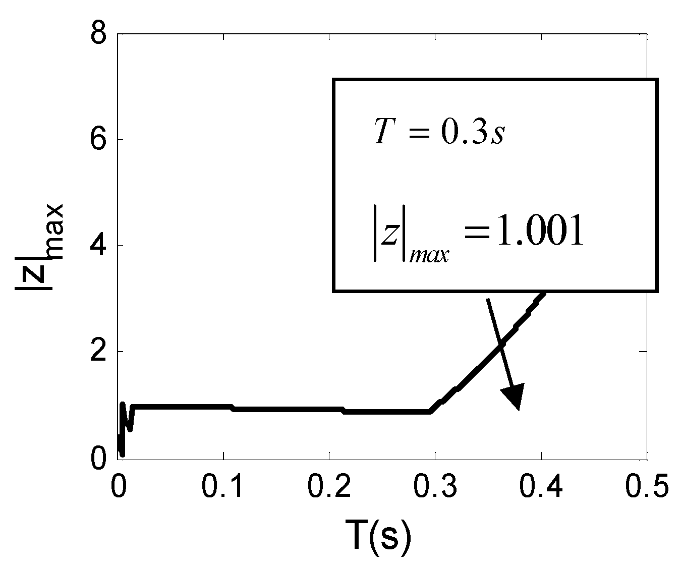
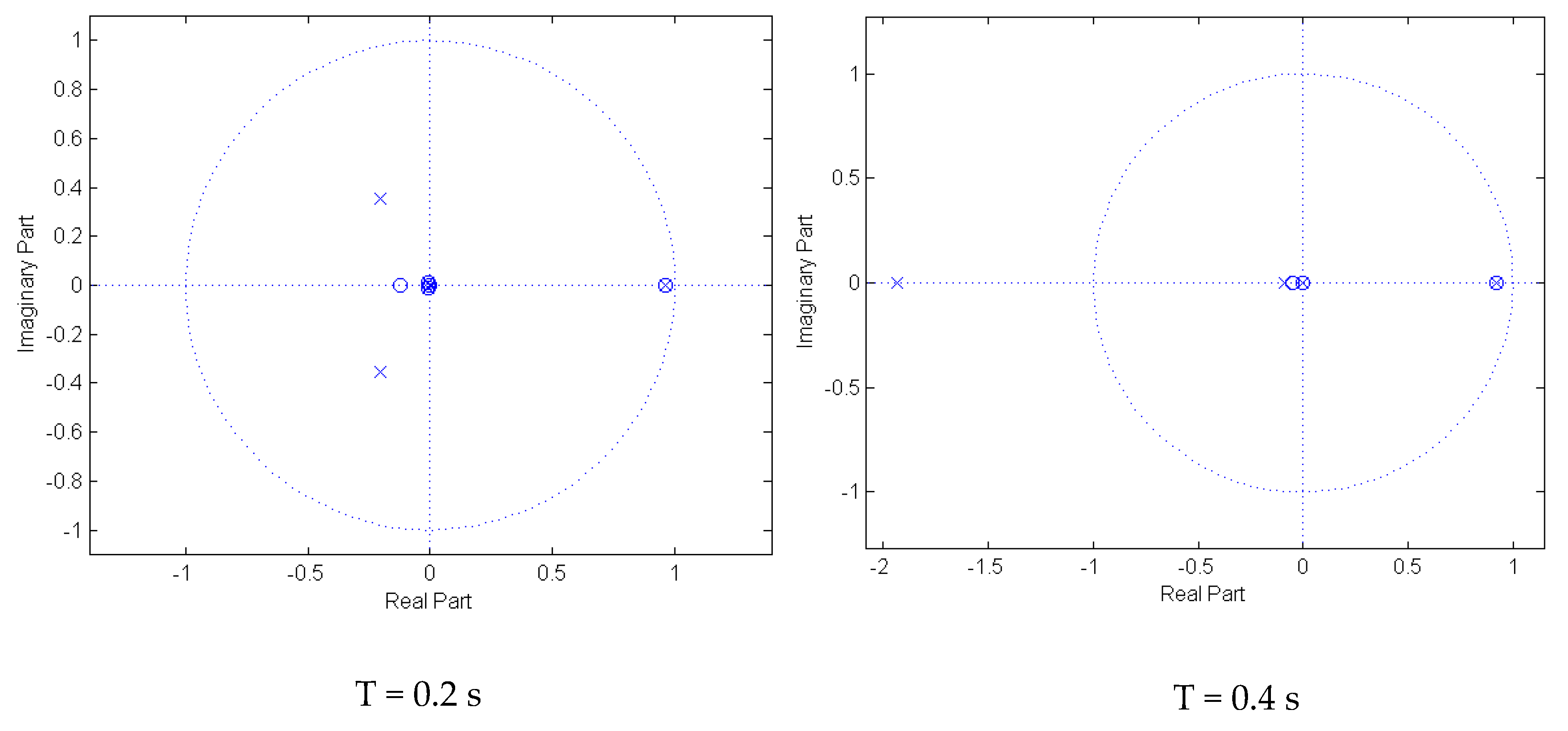
According to the stability criterion expressed in the Z-domain [29], the control system can be stable once all the poles are inside the unit circle of the Z-plane. Using the parameters of the car listed in

Table 1. Parameters used in the stability analysis.

Symbol	Value	Symbol	Value	Symbol	Value
$J_e$	0.1 kg·m2	$J_{c1}$	0.5 kg·m2	$J_{c2}$	0.5 kg·m2
$J_v$	10 kg·m2	$k_e$	1000 Nm/rad	$k_v$	10,000 Nm/rad
$c_e$	10 kg·m2	$c_v$	20 kg·m2	$k_p$	5
$k_i$	1	$\tau$	10 ms

[6], the scheduling periods of T = 0.2 s and 0.4 s are given as examples to show the derivation process of the poles. Then, additional calculations for different scheduling periods are performed. The path of the poles changing with respect to the task scheduling period $T$ is illustrated in Figure 4.

Let T = 0.2 s. Then, the open-loop transfer function $H(z)$ in (21) is calculated as follows.

$$H(z)=\frac{1.439z^6-1.179z^5-0.1924z^4-0.003649z^3-2.88\cdot {10}^{-5}{z}^2+1.785\cdot {10}^{-9}z-1.345\cdot {10}^{-14}}{z^7-1.972z^6+0.9451z^5+0.02713z^4+0.0002246z^3-2.398\cdot {10}^{-9}{z}^2+8.489\cdot {10}^{-15}z}$$

(24)

The seven poles of the closed-loop transfer function $G(z)$ in (22) are calculated as follows.

$$\begin{array}{l}{z}_1=8.78\cdot {10}^{-6},z_2=5.28\cdot {10}^{-5},z_3=0.959\\ z_4=-0.203-0.355\cdot i\\ z_5=-0.203+0.355\cdot i\\ z_6=-0.011-0.008\cdot i\\ z_7=-0.011+0.008\cdot i\end{array}$$

(25)

There are three real poles and four conjugate poles. As shown in Figure 5, it can be seen that the modules of the seven roots are all less than 1, i.e., they are all located inside the unit circle in the Z-plane. Thus, the closed-loop system is stable.

Next, let T = 0.4 s. The open-loop transfer function $H(z)$ in (21) is derived as follows.

$$H(z)=\frac{3.1z^6-2.693z^5-0.1553z^4+2.854\cdot {10}^{-5}{z}^3-6.524\cdot {10}^{-9}{z}^2+1.014\cdot {10}^{-18}z-1.142\cdot {10}^{-28}}{z^7-2z^6+1.001z^5-0.0003118z^4+5.057\cdot {10}^{-8}{z}^3-1.938\cdot {10}^{-18}{z}^2+7.206\cdot {10}^{-29}z}$$

(26)

The seven poles of the closed-loop transfer function $G(z)$ in (22) are calculated as follows.

$$\begin{array}{l}{z}_1=-1.933,z_2=-0.087,z_3=0.921\\ z_4=9.19\cdot {10}^{-5}-1.83\cdot {10}^{-4}\cdot i\\ z_5=9.19\cdot {10}^{-5}+1.83\cdot {10}^{-4}\cdot i\\ z_6=7.77\cdot {10}^{-11}-1.07\cdot {10}^{-10}\cdot i\\ z_7=7.77\cdot {10}^{-11}+1.07\cdot {10}^{-10}\cdot i\end{array}$$

(27)

Again, there are three real poles and four conjugate poles. However, as shown in Figure 5, the first pole $z_1$ is located outside the unit circle in the Z-plane; thus, the closed-loop system is unstable.

Additional calculations for 0.001 s ≤ T ≤ 0.5 s are performed every 0.001 s. The changing path of the maximum module ${\left|z\right|}_{\mathit{max}}$ of the seven poles is plotted in Figure 4. It can be seen that ${\left|z\right|}_{\mathit{max}}$ < 1 when T < 0.3 s, while ${\left|z\right|}_{\mathit{max}}$ > 1 when T > 0.3 s. Therefore, the critical period, represented by $T_{\max }$, is defined as T = 0.3 s. That is, the closed-loop system will be stable when the task scheduling period is T < 0.3 s, whereas it becomes unstable when the task scheduling period is T < 0.3 s.

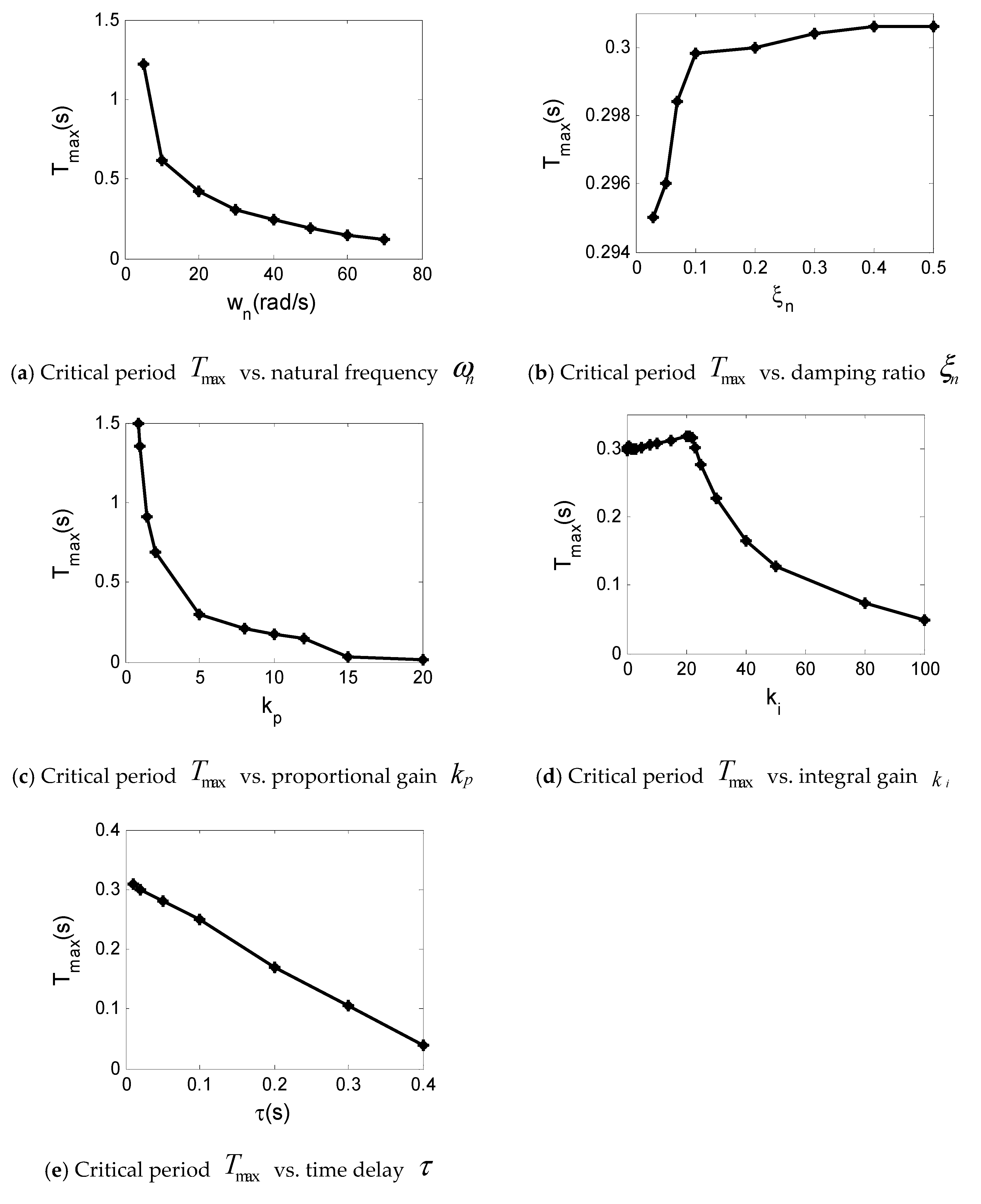
3.4. Sensitivity Analysis

It is of interest that the critical period $T_{\max }$ may be sensitive to some parameters. The key parameters of the three subsystems other than the zero-order holder of the overall system, as shown in Figure 2, were selected as influencing factors. Regarding the powertrain subsystem, the natural frequency ${\omega }_n$ (defined as $w_n=\sqrt{k_v/J_v}$) and the damping coefficient ${\xi }_n$ (defined as ${\xi }_n=c_v/\sqrt{k_v{J}_v}$) were selected since the two kinetic parameters are related to one performance evaluation index of clutch engagement, i.e., vehicle jerk. Regarding the control algorithm subsystem, two control gains, $k_p$ and $k_i$, were selected because they are used in the feedback loop. In addition, the delay $\tau$ was selected from the time delay subsystem. In total, five influencing factors were examined.

Using the data in Table 1, the base values of ${\omega }_n$ and ${\xi }_n$ were calculated to be ${\omega }_n=32 \mathrm{rad}/\mathrm{s}$ and ${\xi }_n=0.32$, respectively. The base values of $k_p$, $k_i$, and the time delay are $k_p=5$, $k_i=1$, and $\tau$ = 0.01 s, respectively, as shown in Table 1. With the other four parameters unchanged, the critical period $T_{\max }$ for task scheduling changes with respect to ${\omega }_n$, ${\xi }_n$, $k_p$, $k_i$, and $\tau$, as shown in Figure 6.

As shown in Figure 6a, the critical period $T_{\max }$ decreases with the increase in ${\omega }_n$. As we know that the increase in ${\omega }_n$ means a decrease in the natural oscillation period of the powertrain. Therefore, the critical period $T_{\max }$ decreases as the natural oscillation period decreases, and vice versa. In other words, a shorter oscillation period tolerates a shorter critical period $T_{\max }$.

On the other hand, as shown in Figure 6b, the critical period $T_{\max }$ increases with the increase in the damping ${\xi }_n$. This trend agrees with the common sense that more damping helps to prevent system instability because damping can absorb a lot of vibration energy. Nevertheless, as indicated by the range of $T_{\max }$, the critical period $T_{\max }$ is more sensitive to the natural frequency ${\omega }_n$ than to the damping coefficient ${\xi }_n$.

As shown in Figure 6c,d, the critical period $T_{\max }$ generally decreases with the increase in the gains $k_p$ and $k_i$. In real applications, the two gains are always tuned to large value to obtain a small steady-state error and short settling time. However, the analysis in this study indicates that the two gains should be small when the task scheduling period is large.

As shown in Figure 6e, the critical period $T_{\max }$ decreases with the increase in the delay $\tau$. For the ideal actuation system without a time delay, the critical period is 0.31 s. However, in a real actuation system, time delay is inevitable. Thus, the critical period should be less than 0.31 s in real cases.

A comparison of the sensitivity of the five factors shows that the critical period is the most sensitive to the natural frequency ${\omega }_n$; on the contrary, it is the least sensitive to the damping coefficient ${\xi }_n$. In addition, the critical period is more sensitive to the proportional gain $k_p$ than the integral gain $k_i$. The sensitivity of the time delay $\tau$ is similar to that of the proportional gain $k_p$.

4. Real-Time Test from Slipping to Being Locked Phase

The stability analysis in the first step is useful but does not provide enough information regarding the three phases of the complete engagement process. Due to the transition of the friction state from slipping to being locked, as modeled in (5), a stable slipping phase does not necessarily indicate a smooth transition. Therefore, the second step of the control–scheduling co-design was to perform real-time hardware-in-the-loop tests aiming to examine the influence of the task scheduling period on the clutch engagement performance, especially in regard to the friction state transition.

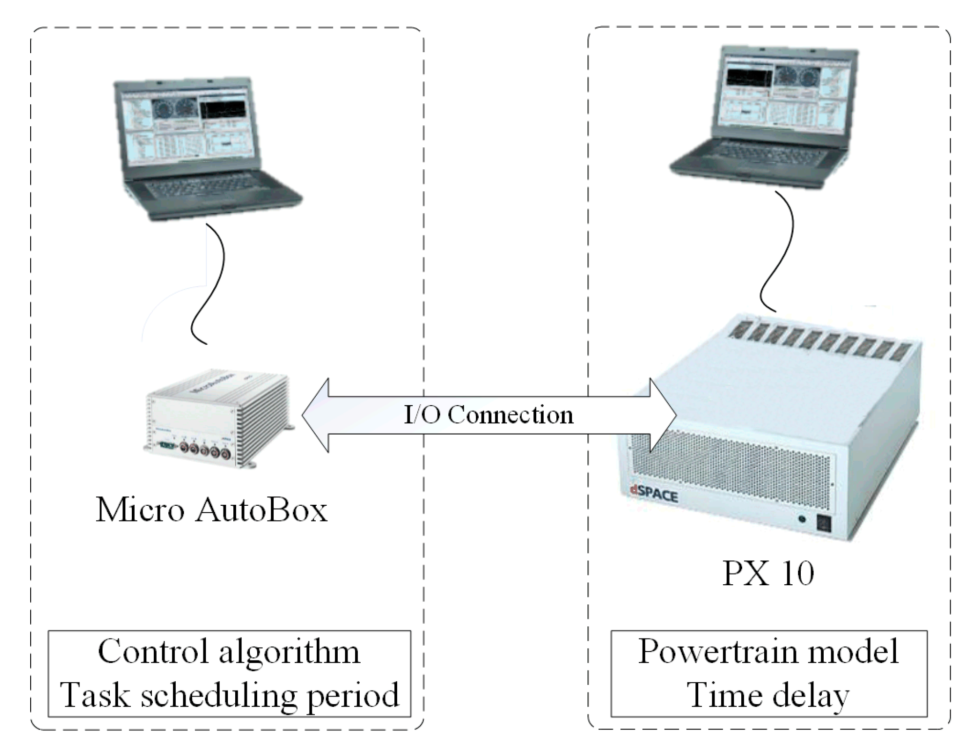
The real-time environment consists of one MicroAutobox and one hardware-in-the-loop device (dSPACE PX10), as shown in Figure 7. The MicroAutobox is used to run the control algorithm and implement the task scheduling period via timer configuration, and the PX10 is used to run the powertrain model and simulate the time delay. The two communicate through a timer-triggered input/output (I/O) connection. Because the time-related settings can be implemented by hardware, the test accuracy can be higher than that of software simulation.

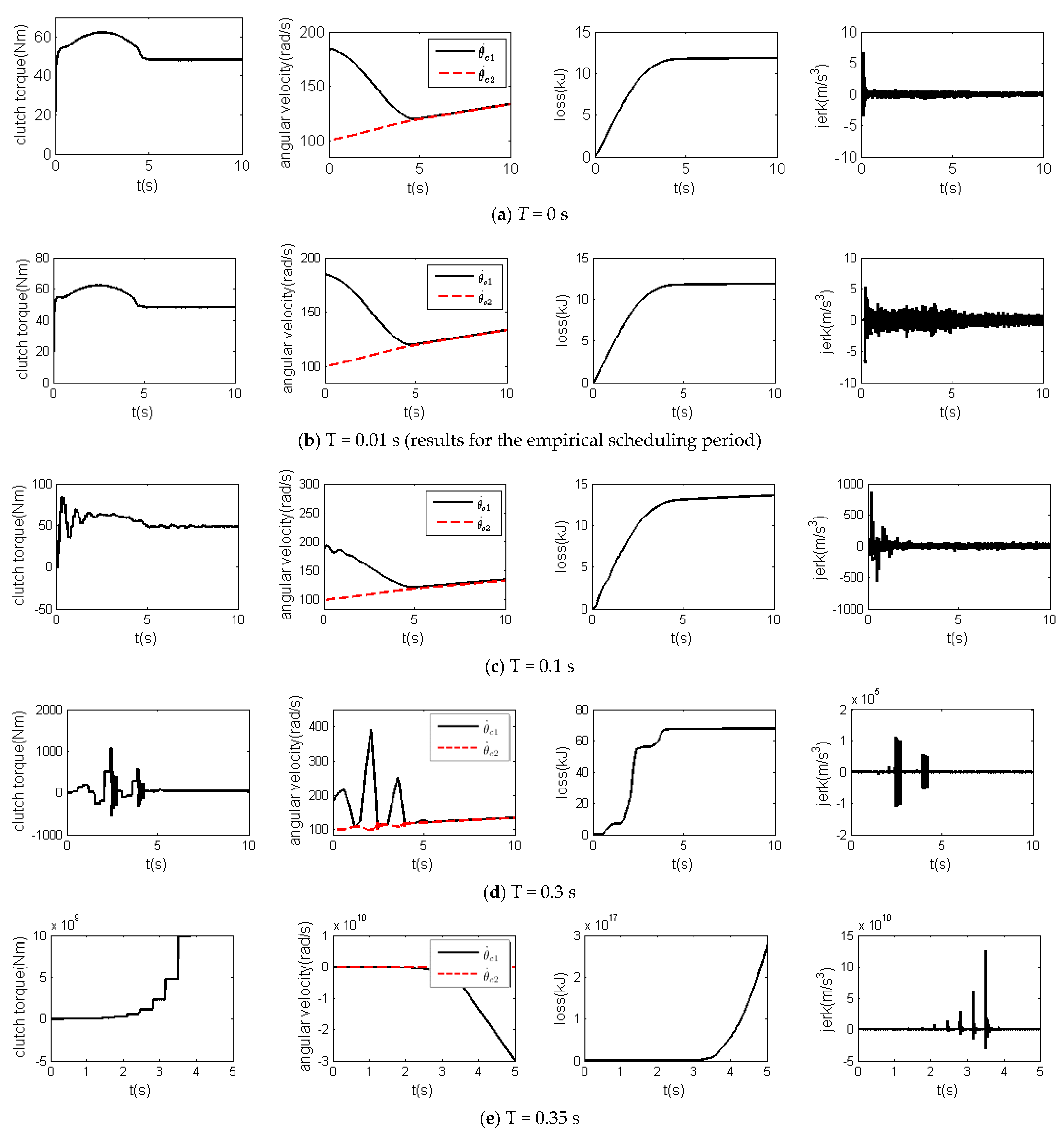
The dynamic responses during the clutch engagement under different task scheduling periods are illustrated in Figure 7, with the engine torque set as a constant (T_e = 50 Nm) and with the car parameters listed in Table 1 and

Table 2. Parameters used in real-time modeling [25].

Symbol	Value	Symbol	Value	Symbol	Value
$m$	1600 kg	$R_c$	0.15 m	${\mu }_s$	0.44
$\mu$	0.4	$c_D$	0.32	$A_V$	1.8 m2
${\rho }_{air}$	1.205 kg/m3	$f$	0.0015	$R$	0.32 m
$N$	2	${{\displaystyle i}}_g$	3.5

[25].

Regarding the control–scheduling co-design, there are three kinds of evaluation methods. The first describes the evaluation index as a function of the task scheduling period [30,31]. The second defines the execution deadline for the control task, which represents the worst case [32,33]. Obviously, neither of these reflect the dynamic response affected by the task scheduling period. The third type of method employs dynamic characteristics, such as the stability, vibration, or response time, according to the state equations or transfer functions of the control plant [19,34]. In this study, the third method is used to evaluate the clutch engagement performance with regard to the vehicle jerk and frictional loss.

The vehicle jerk describes the smoothness of the running vehicle, which is a derivative of the vehicle acceleration. The frictional loss represents the energy dissipation during the engagement process, which is calculated as follows.

$$E_D={\displaystyle {\int }_{t_1}^{t_2}\left|({\dot{\theta }}_{c1}-{\dot{\theta }}_{c2})\cdot T_c\right|}\mathrm{d}t$$

(28)

The test results for the six cases are illustrated in Figure 8. The first one is the continuous case without considering the task scheduling period, represented by T = 0 s. Additionally, three typical scheduling periods were selected around the critical period, as shown in the figure: T = 0.1 s, 0.3 s, and 0.35 s. To better understand the significance of the proposed method, the results for the empirical scheduling period (T = 0.01 s) typically used in engineering are provided for comparison.

The results for the continuous case (T = 0 s) are shown as the benchmark in Figure 8a. The control input, i.e., the clutch transmitted torque $T_c$, gradually increases and decreases before synchronization. The clutch is slipping in this phase, and the magnitude of the clutch transmitted torque $T_c$ is proportional to the normal force on the friction plates. After synchronization, the normal force is actuated to maximum, but the clutch transmitted torque $T_c$ is determined by the input torque and load torque of the powertrain so that it is less than that in the slipping phase. It can be seen that the driving and driven parts of the clutch can slip and synchronize smoothly, and the vehicle jerk is almost imperceptible. The clutch torque $T_c$ gradually increases and decreases before synchronization. Since the transmitted torque $T_c$ has a direct effect on the powertrain dynamics, the profile of $T_c$ is given. These results are ideal for clutch engagement control.

The results for the empirical case (T = 0.01 s) are illustrated in Figure 8b. It can be observed that the angular velocity of the driving part grows faster than that for the continuous case at the beginning of the engagement. Thus, the slipping velocity is higher, and the transient clutch torque is larger according to (13). Thereafter, the transient vehicle jerk is more intense, and the frictional loss is greater than those of the continuous case. Nevertheless, the driving and driven parts of the clutch can synchronize after slipping, and the vehicle jerk is <10 m/s³. The engagement performance is acceptable. Thus, the test results were validated by the empirical results.

When the task scheduling period increases to T = 0.1 s, which still falls into the stable region of T < 0.3 s, the control input $T_c$ is obviously in a step shape, owing to the discretization and zero-order hold, as shown in Figure 8c. In addition, the control input $T_c$ oscillates between positive and negative values, because $e(t)$ in (13) is positive and negative. The torque $T_c$ affects the dynamic response of the clutch driving part and driven part simultaneously according to (1)–(4). Because the inertia moment of the driving part ($J_e$ and $J_{c1}$) is significantly lower than that of the driven part ($J_{c2}$ and $J_v$), the oscillation of the driving part (as indicated by ${{\displaystyle \dot{\theta }}}_{c1}$) induced by the discretized $T_c$ is evident, and is more intense than that of the driven part (as indicated by ${{\displaystyle \dot{\theta }}}_{c2}$). Nevertheless, the clutch can complete the synchronization at the end of the engagement. The effect of the discretized $T_c$ on the clutch-driven part, which is also called the vehicle-body part, is reflected by vehicle jerk. The vehicle jerk is greater than 850 m/s³ in the slipping stage. Such intense jerking is harmful to the powertrain components and reduces the comfort of the vehicle passengers.

When the task scheduling period increases to T = 0.3 s, which is at the critical boundary, the oscillation of the clutch driving part is significantly more intense than that in the previous two cases, as shown in Figure 8d. The amplitude of the control input $T_c$ increases from approximately 200 to 1000 Nm owing to the large error in the slipping velocity. Stick-slip motions can be observed, which are not expected in a smooth engagement process. Because of the oscillation induced by discretization with the scheduling period at the critical boundary, the vehicle jerk is greater than 1 × 10⁵ m/s³, and the frictional loss is greater than 60 kJ.

When the task scheduling period increases to T = 0.35 s, which falls into the unstable region of T > 0.3 s, the dynamic response is divergent, as shown in Figure 8e, and the clutch synchronization fails.

From the above, the critical scheduling period (T = 0.3 s) cannot satisfy the control performance evaluated in terms of the vehicle jerk. A sub-boundary may exist. The control performance can be satisfied when the scheduling period is within the sub-boundary, for example, the empirical scheduling period of T = 0.1 s.

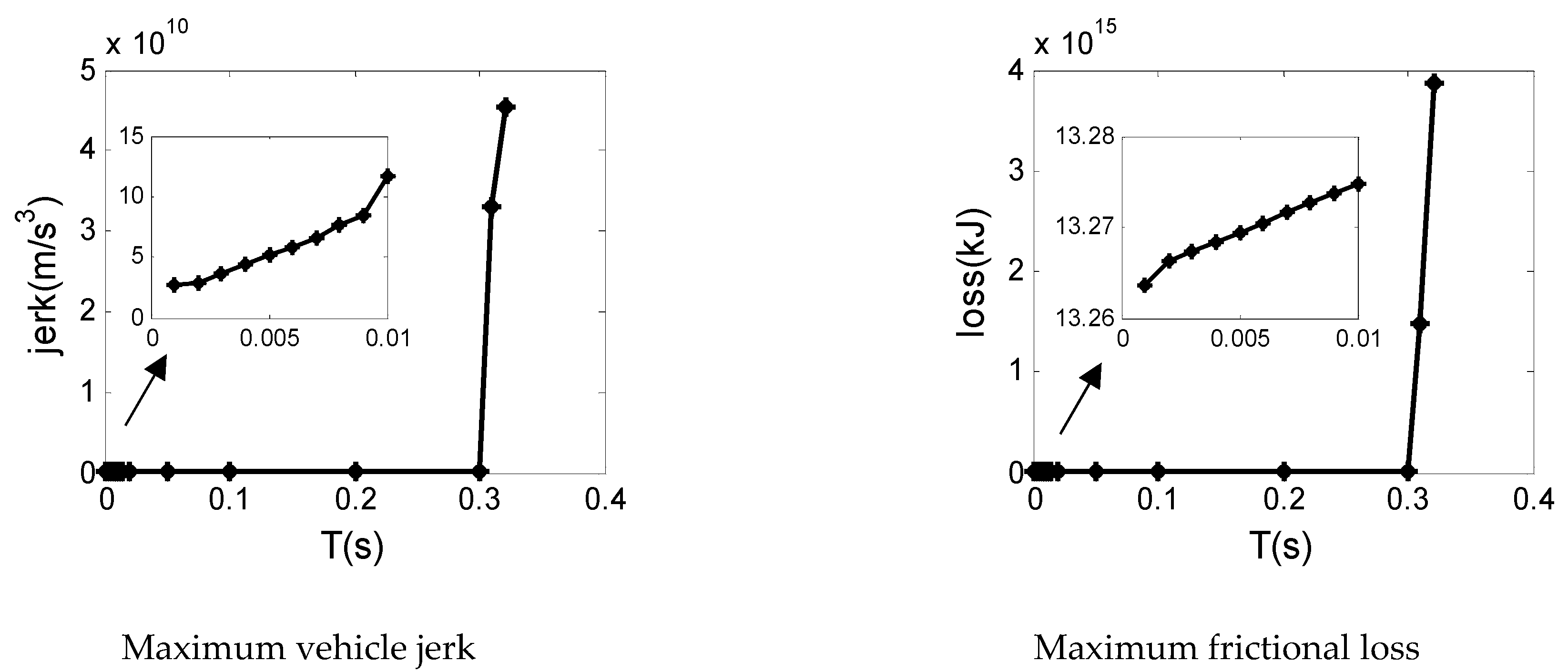
As shown in Figure 9, in order to find the sub-boundary, tests for the task scheduling period T ranging from 0.001 to 0.32 s are performed every 0.001 s. The test runs for 10 s in each case. The vehicle jerk is calculated, and the maximum value is recorded. The evolution of the maximum vehicle jerk and frictional loss with respect to the task scheduling period is plotted in Figure 8. It can be seen that the maximum vehicle jerk and frictional loss increase rapidly when the task scheduling period $T$ is longer than 0.3 s, which is the critical period that separates the stable and unstable regions. When the task scheduling period $T$ is less than 0.3 s, the rate of increase is rather low. In particular, the maximum vehicle jerk is less than 10 m/s³ when the task scheduling period is in the range of T < 0.01 s. Therefore, the sub-boundary here is 0.01 s.

The influence of the task scheduling period is summarized in

Table 3. Summary of the influence of the task scheduling period on the engagement performance.

	T < 0.01 s	0.01 s ≤ T ≤ 0.30 s	T > 0.30 s
Average increasing rate of vehicle jerk (m/s4)	7.1 × 102	1.6 × 105	2.3 × 1012
Average increasing rate of frictional loss (J/s)	1.2 × 103	2.7 × 105	1.9 × 1020

. The critical period obtained in the first step is significant for the whole process because it is an obvious turning point in terms of the clutch engagement performance. As seen from the real-time hardware-in-the-loop test results, the critical period for the clutch engagement process is 0.30 s. Furthermore, as a practical reference, the scheduling period should be selected within the sub-boundary, which is 0.01 s, so as to realize a smooth engagement process.

5. Conclusions

This paper proposes a systematic control–scheduling co-design methodology for selecting the task scheduling period for clutch engagement control. The co-design has two steps. In the first step, stability analysis is conducted for the slipping phase based on a linearized system model enveloping the driving and driven part of the clutch, feed-forward and feedback control loop together with a zero-order signal holder. The critical period is determined according to pole locations. The evolution of the critical period with respect to five key parameters—the natural frequency, damping coefficient, proportional gain, integral gain, and time delay—is illustrated. In the second step, hardware-in-the-loop experiments are performed in a dSPACE real-time environment to inspect the dynamic response concerning the friction state transition. The results show that the critical period identified in the first step can induce intensive slip-stick motion and it represents a turning point in terms of clutch engagement performance. Specifically, the vehicle jerk and clutch frictional loss generally increase with the increase in the scheduling period. When the scheduling period is shorter than the critical period, the rate of increase is mild. However, once the scheduling period exceeds the critical period, the rate of increase becomes very high. Furthermore, a sub-boundary of the scheduling period is found to guarantee the control performance to satisfy the engineering requirements.

The proposed methodology provides a useful reference for the design of clutch control systems, especially for the case of the advanced optimal control algorithm that requires a predefined task scheduling period. The methodology can also be extended to other industrial applications that employ electronic controllers.

References

- Xiong, W.; Zhang, Y.; Yin, C. Optimal energy management for a series–parallel hybrid electric bus. Energy Convers. Manag. 2009, 50, 1730–1738. [Google Scholar] [CrossRef]
- Chao, Y.; Jian, S.; Liang, L.; Li, S.; Cao, D. Economical launching and accelerating control strategy for a single-shaft parallel hybrid electric bus. Mech. Syst. Signal Process. 2016, 76, 649–664. [Google Scholar]
- Vasca, F.; Iannelli, L.; Senatore, A.; Reale, G. Torque Transmissibility Assessment for Automotive Dry-Clutch Engagement. IEEE/ASME Trans. Mechatron. 2010, 16, 564–573. [Google Scholar] [CrossRef]
- Chen, L.; Xi, G. Stability and response of a self-amplified braking system under velocity-dependent actuation force. Nonlinear Dyn. 2014, 78, 2459–2477. [Google Scholar] [CrossRef]
- Chen, L.; Liu, F.; Yao, J.; Ding, Z.; Lee, C.; Kao, C.-K.; Samie, F.; Huang, Y.; Yin, C. Design and validation of clutch-to-clutch shift actuator using dual-wedge mechanism. Mechatronics 2017, 42, 81–95. [Google Scholar] [CrossRef]
- Liu, F.; Chen, L.; Li, D.; Yin, C. Improved clutch slip control for automated transmissions. Proc. Inst. Mech. Eng. Part C J. Mech. Eng. Sci. 2017, 232, 3181–3199. [Google Scholar] [CrossRef]
- Yao, J.; Chen, L.; Liu, F.; Yin, C. Experimental study on improvement in the shift quality for an automatic transmission using a motor-driven wedge clutch. Proc. Inst. Mech. Eng. Part D J. Automob. Eng. 2014, 228, 663–673. [Google Scholar] [CrossRef]
- Li, D.; Liu, L.; Liu, Y.-J.; Tong, S.; Chen, C.L.P. Fuzzy Approximation-Based Adaptive Control of Nonlinear Uncertain State Constrained Systems with Time-Varying Delays. IEEE Trans. Fuzzy Syst. 2019, 28, 1620–1630. [Google Scholar] [CrossRef]
- Tafti, H.D.; Sangwongwanich, A.; Yang, Y.; Pou, J.; Konstantinou, G.; Blaabjerg, F. An Adaptive Control Scheme for Flexible Power Point Tracking in Photovoltaic Systems. IEEE Trans. Power Electron. 2019, 34, 5451–5463. [Google Scholar] [CrossRef] [Green Version]
- Huang, T.; Yang, K.; Zhu, Y.; Tang, Q.; Cheng, M.; Wang, Y. LFT-Structured Uncertainty State-Space Modeling for State Feedback Robust Control of the Ultra-Precision Wafer Stage. IEEE Trans. Ind. Electron. 2019, 66, 8567–8577. [Google Scholar] [CrossRef]
- Wang, T.; Zhang, Y.; Chen, Z.; Zhu, S. Parameter Identification and Model-Based Nonlinear Robust Control of Fluidic Soft Bending Actuators. IEEE/ASME Trans. Mechatron. 2019, 24, 1346–1355. [Google Scholar] [CrossRef]
- Gu, K. A further refinement of discretized Lyapunov functional method for the stability of time-delay systems. Int. J. Control 2001, 74, 967–976. [Google Scholar] [CrossRef]
- Wang, B.; Yu, X.; Li, X. ZOH Discretization Effect on Higher-Order Sliding-Mode Control Systems. IEEE Trans. Ind. Electron. 2008, 55, 4055–4064. [Google Scholar] [CrossRef]
- Liu, J.; Peng, B.; Zhang, T. Effect of discretization on dynamical behavior of SEIR and SIR models with nonlinear incidence. Appl. Math. Lett. 2015, 39, 60–66. [Google Scholar] [CrossRef]
- Wu, Y.; Buttazzo, G.; Bini, E.; Cervin, A. Parameter Selection for Real-Time Controllers in Resource-Constrained Systems. IEEE Trans. Ind. Inform. 2010, 6, 610–620. [Google Scholar] [CrossRef]
- Aydin, H.; Melhem, R.; Mosse, D.; Mejfa-Alvarez, P. Optimal reward-based scheduling of periodic real-time tasks. IEEE Trans. Comput. 2003, 1, 50. [Google Scholar] [CrossRef] [Green Version]
- Mayank, J.; Mondal, A.; Sarkar, A. Control-schedule co-design for fast stabilization in real time systems facing repeated reconfigurations. Des. Autom. Embed. Syst. 2019, 23, 79–101. [Google Scholar] [CrossRef]
- Wang, T.; Zhou, C.; Hui, L.; He, J.; Jian, G. Hybrid Scheduling and Quantized Output Feedback Control for Networked Control Systems. Int. J. Control. Autom. Syst. 2018, 16, 197–206. [Google Scholar] [CrossRef]
- Dai, S.-L.; Lin, H.; Ge, S.S. Scheduling-and-Control Codesign for a Collection of Networked Control Systems with Uncertain Delays. IEEE Trans. Control Syst. Technol. 2009, 18, 66–78. [Google Scholar] [CrossRef]
- Cervin, A.; Velasco, M.; Marti, P.; Camacho, A. Optimal Online Sampling Period Assignment: Theory and Experiments. IEEE Trans. Control Syst. Technol. 2011, 19, 902–910. [Google Scholar] [CrossRef]
- Min, Z.; Jin, W.; Ma, A. Co-design of optimal feedback scheduling strategy and fault detection for networked control systems. In Proceedings of the 2016 IEEE Chinese Guidance, Navigation and Control Conference (CGNCC), Nanjing, China, 12–14 August 2016; pp. 216–221. [Google Scholar]
- Yun, N.; Liang, Y.; Yang, H. Event-triggered robust control and dynamic scheduling co-design for networked control system. In Proceedings of the 2017 14th International Bhurban Conference on Applied Sciences and Technology (IBCAST), Islamabad, Pakistan, 10–14 January 2017; pp. 237–243. [Google Scholar]
- Wen, S.; Guo, G.; Wong, W.S. Hybrid event-time-triggered networked control systems: Scheduling-event-control co-design. Inf. Sci. 2015, 305, 269–284. [Google Scholar] [CrossRef]
- ArnellP, R.D.; Davies, B.; Halling, J.; Whomes, T.L. Tribology: Principles and Design Applications, 1st ed.; Springer: Berlin/Heidelberg, Germany, 1991. [Google Scholar]
- Chen, L.; Xi, G.; Sun, J. Torque Coordination Control During Mode Transition for a Series–Parallel Hybrid Electric Vehicle. IEEE Trans. Veh. Technol. 2012, 61, 2936–2949. [Google Scholar] [CrossRef]
- Wang, X.; Li, L.; Yang, C. Hierarchical Control of Dry Clutch for Engine-Start Process in a Parallel Hybrid Electric Vehicle. IEEE Trans. Transp. Electrif. 2016, 2, 231–243. [Google Scholar] [CrossRef]
- Zhang, J.; Chen, L.; Xi, G. System dynamic modelling and adaptive optimal control for automatic clutch engagement of vehicles. Proc. Inst. Mech. Eng. Part D J. Automob. Eng. 2002, 216, 983–991. [Google Scholar] [CrossRef]
- Chen, Y.; Wang, X.; He, K.; Yang, C. Model reference self-learning fuzzy control method for automated mechanical clutch. Int. J. Adv. Manuf. Technol. 2016, 94, 3163–3172. [Google Scholar] [CrossRef]
- Dorf, C.R.; Bishop, R. Modern Control Systems, 7th ed.; Pearson Prentice Hall: Hoboken, NJ, USA, 1994. [Google Scholar]
- Seto, D.; Lehoczky, J.P.; Sha, L.; Shin, K.G. On task schedulability in real-time control systems. In Proceedings of the 17th IEEE Real-Time Systems Symposium, Washington, WA, USA, 4–6 December 1996; pp. 13–21. [Google Scholar] [CrossRef]
- Bini, E.; Natale, M.D. Optimal Task Rate Selection in Fixed Priority Systems. In Proceedings of the IEEE International Real-Time Systems Symposium, Miami, FL, USA, 5–8 December 2005; pp. 399–409. [Google Scholar]
- Balbastre, P.; Ripoll, I.; Crespo, A. Optimal deadline assignment for periodic real-time tasks in dynamic priority systems. In Proceedings of the Euromicro Conference on Real-Time Systems, Dresden, Germany, 5–7 July 2006. [Google Scholar] [CrossRef]
- Hoang, H.; Buttazzo, G.; Jonsson, M.; Karlsson, S. Computing the Minimum EDF Feasible Deadline in Periodic Systems. In Proceedings of the IEEE International Conference on Embedded and Real-Time Computing Systems and Applications, Sydney, Australia, 16–18 August 2006; pp. 125–134. [Google Scholar]
- Reimann, S.; Wu, W.; Liu, S. Real-Time Scheduling of PI Control Tasks. IEEE Trans. Control. Syst. Technol. 2015, 24, 1118–1125. [Google Scholar] [CrossRef]
Figure 1.
Two-step framework of the proposed control–scheduling co-design.
Figure 2.
Diagram of closed-loop control system during clutch engagement.