
Adaptive Volt–Var Control in Smart PV Inverter for Mitigating Voltage Unbalance at PCC Using Multiagent Deep Reinforcement Learning


Abstract
:1. Introduction
2. Problem Formulation
2.1. Voltage Unbalance Factors and Sequence Voltage
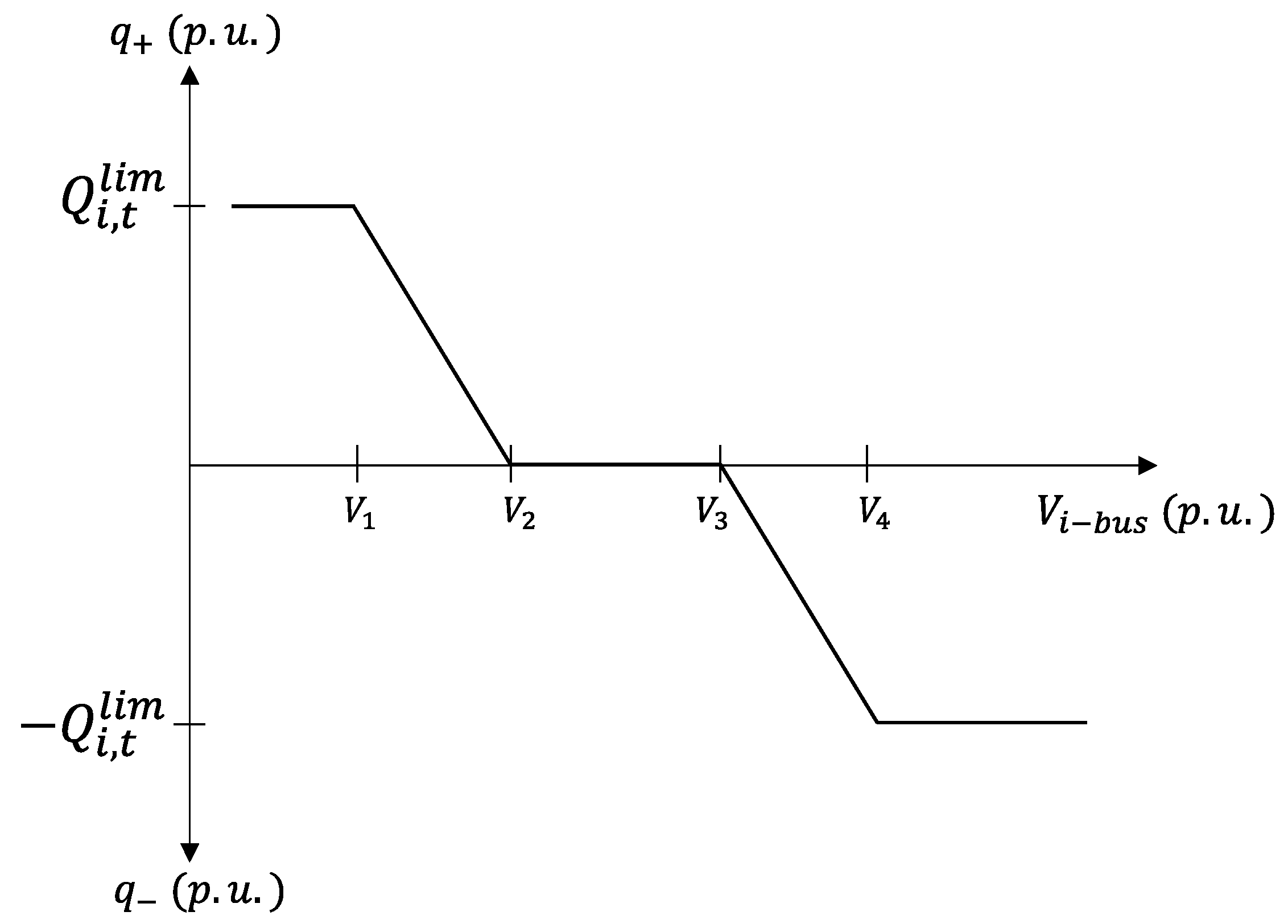
2.2. Volt–Var Curve
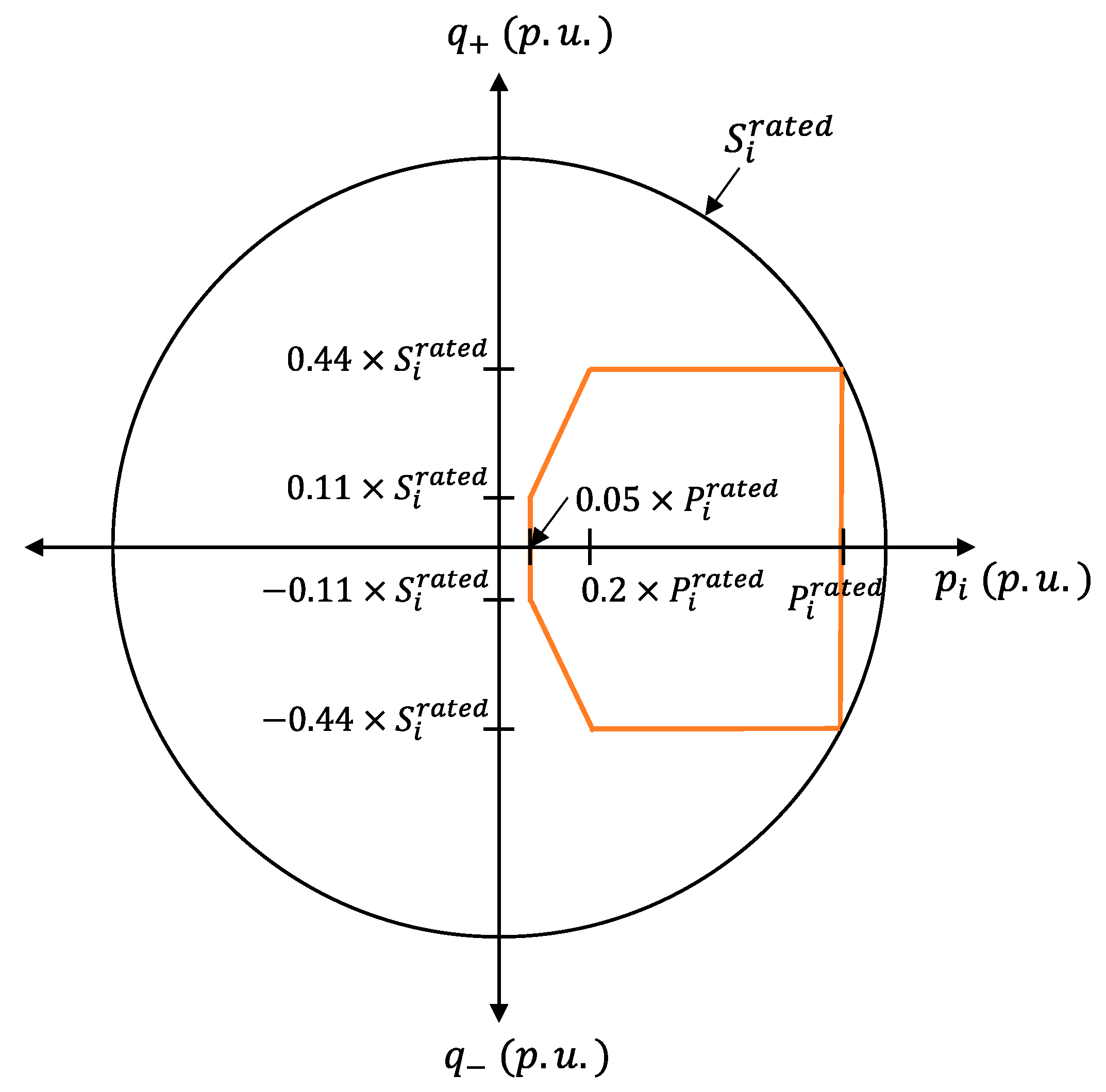
2.3. Reactive Power Capability
3. Multiagent DRL Design for Proposed Method
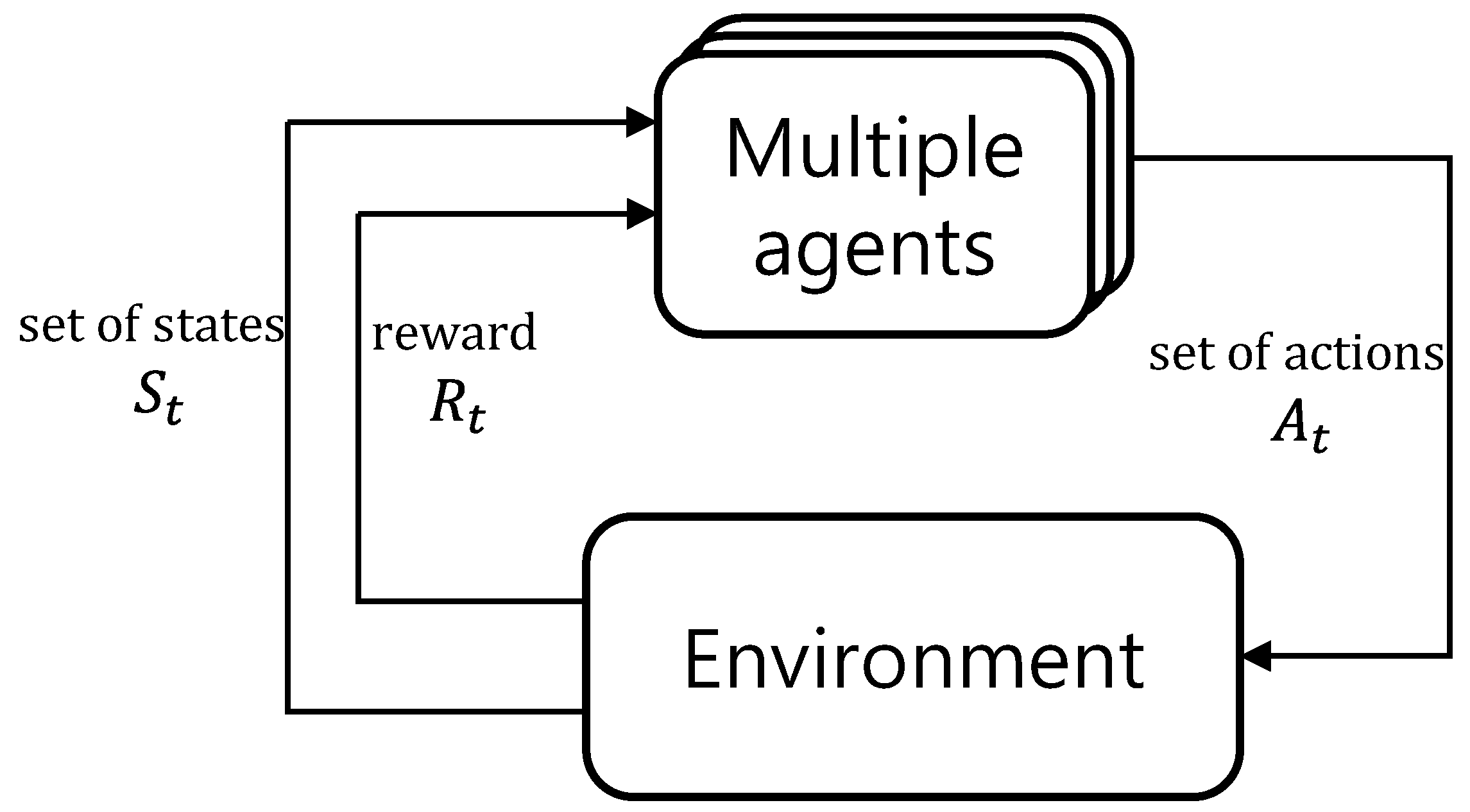
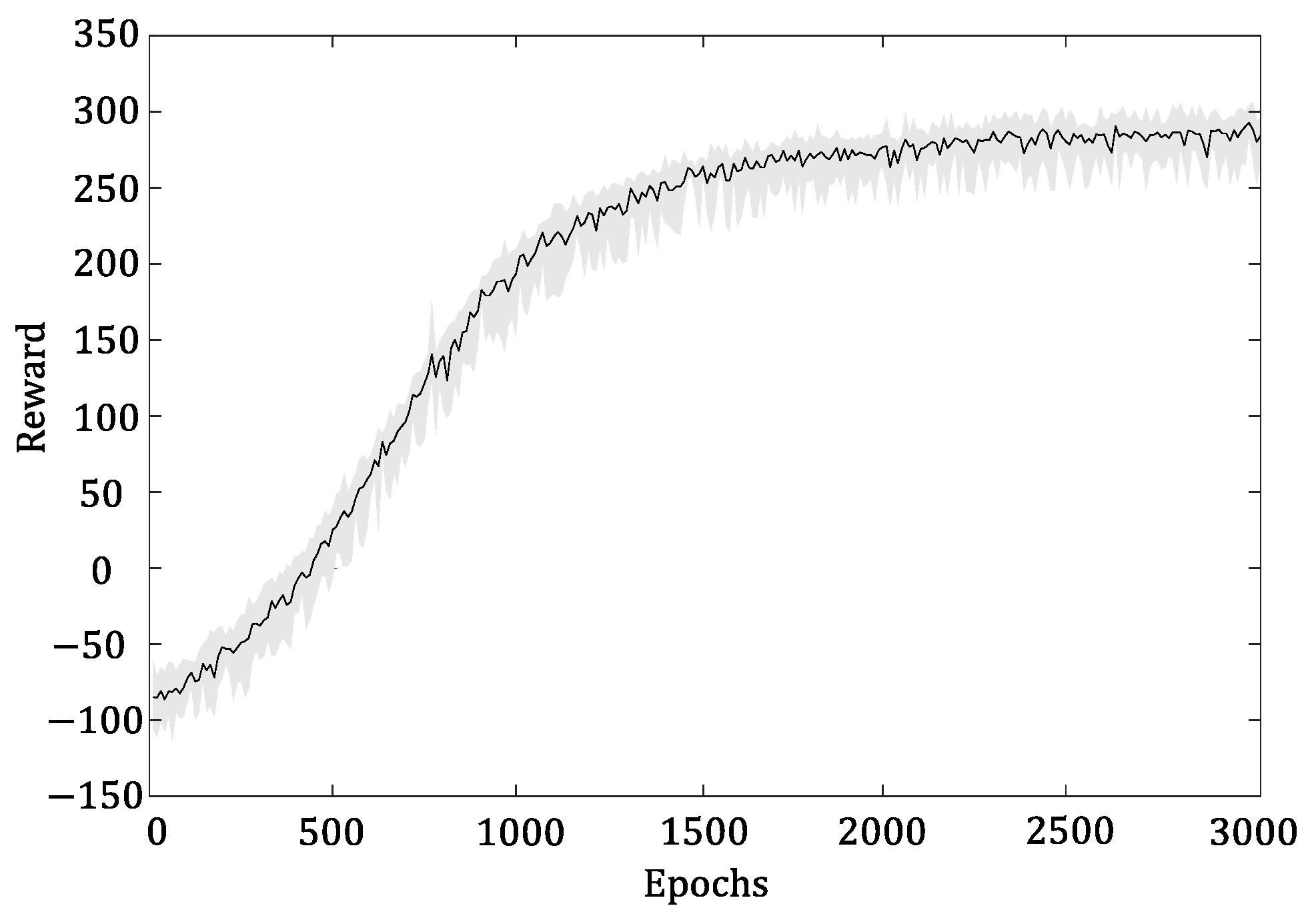
3.1. Principles of Deep Reinforcement Learning
3.2. Proximal Policy Optimization
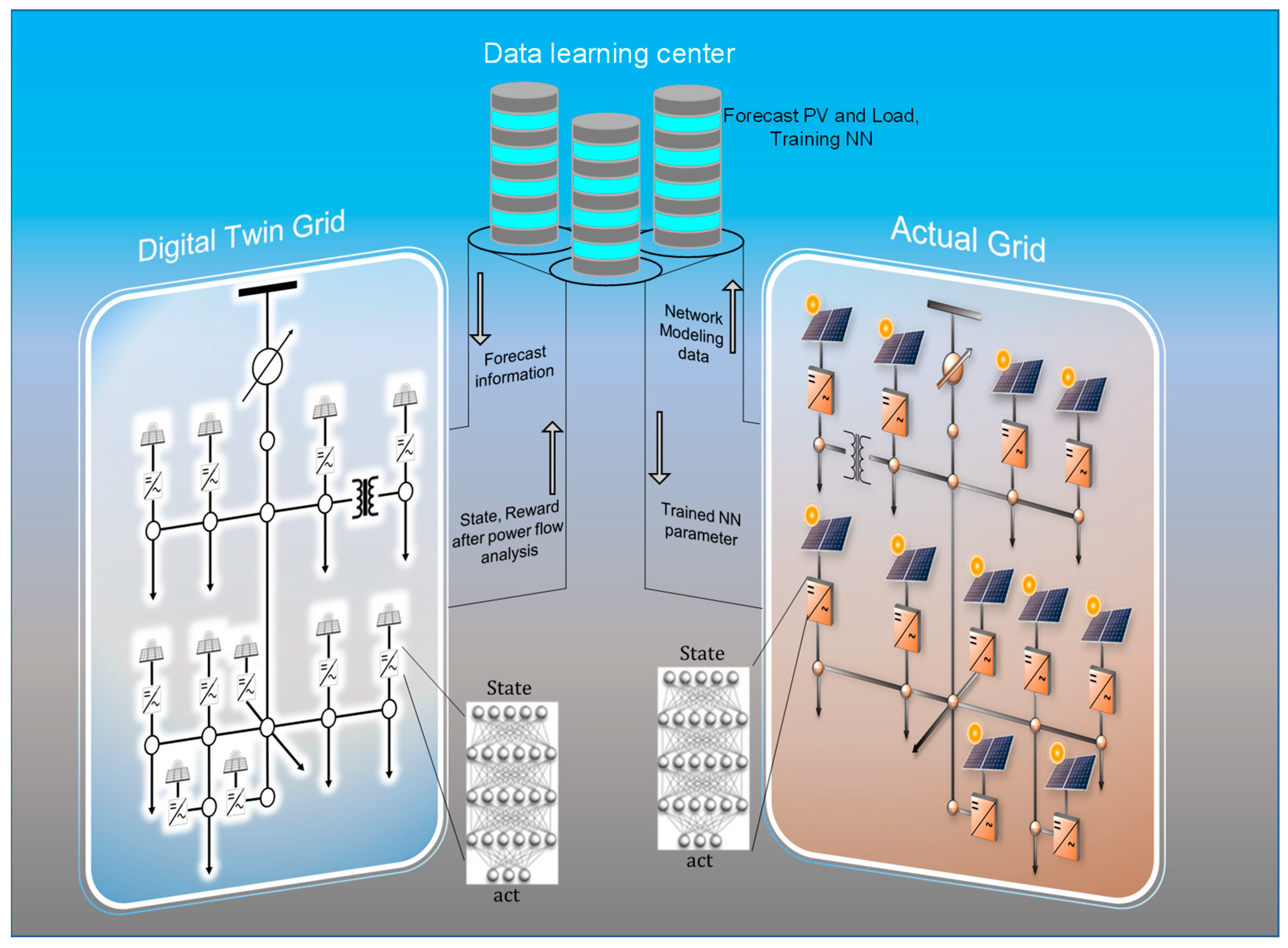
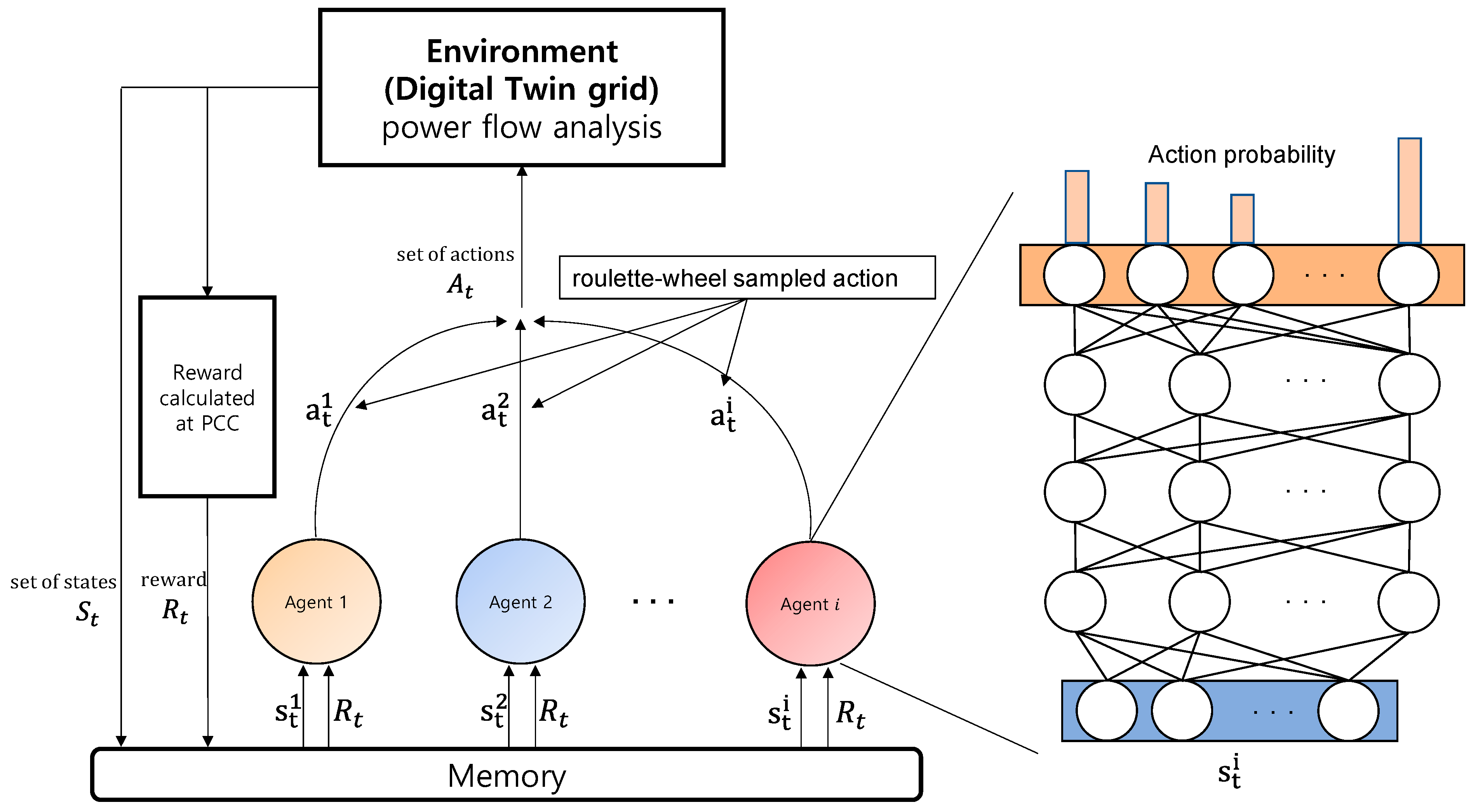
3.3. PPO-Based Multiagent DRL Framework for Autonomous Control
3.3.1. State
3.3.2. Action
3.3.3. Reward
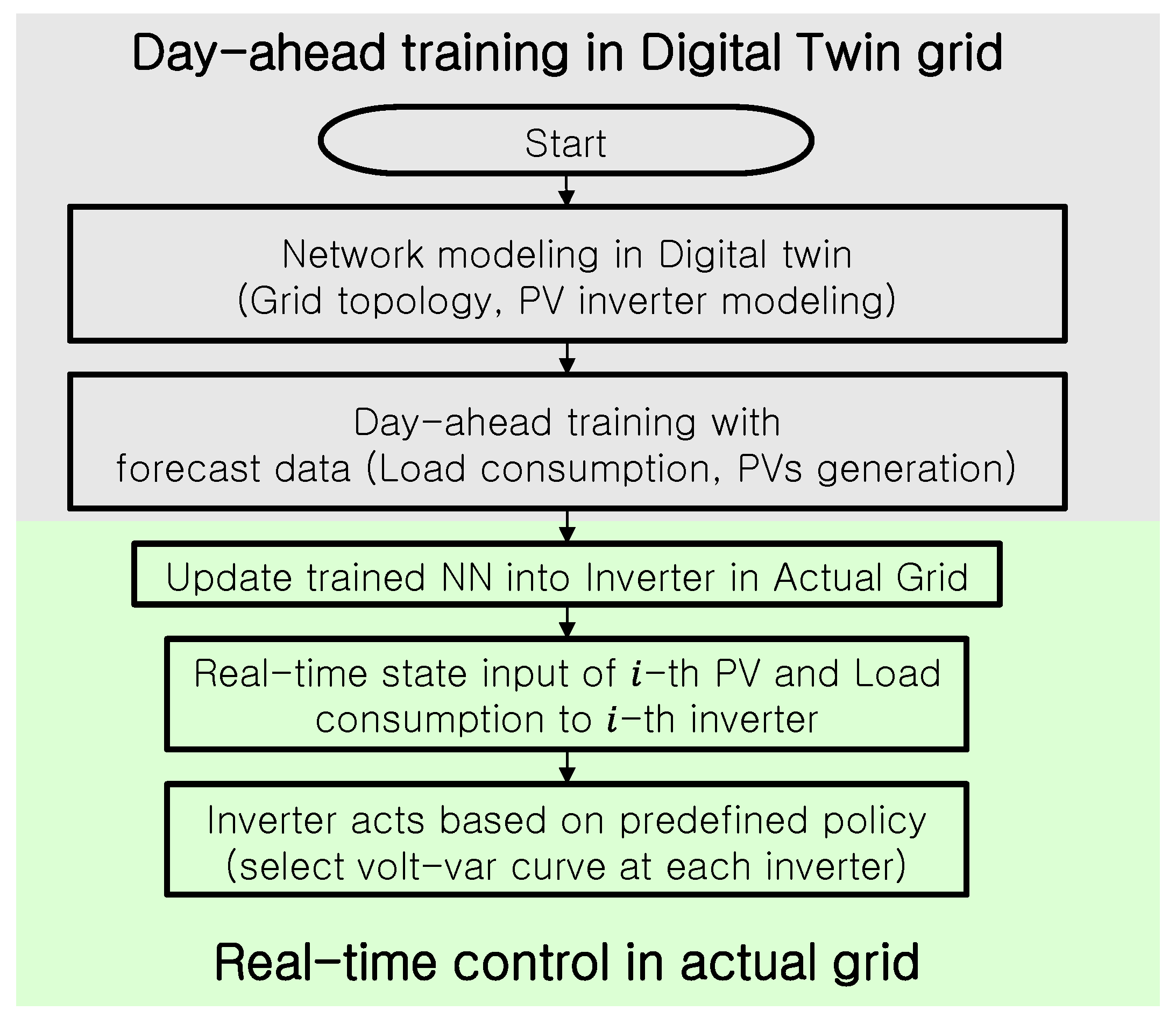
3.4. Proposed Algorithm
| Algorithm 1. Training algorithm based on PPO. |
| 1: Initialize network |
| 2: Initialize the critic and actor networks with weights |
| 3: for episode = 1 to N do |
| 4: for time step = 360 min (6 h) to 1200 min (20 h) do |
| 5: each agent selects an action for each |
| 6: Execute in environment |
| 7: for time step = 0 s (0 min) to 60 s (1 min) do |
| 8: Solve power flow with proposed volt–var curve |
| 9: Calculate at PCC |
| 10: Solve power flow with fixed volt–var curve |
| 11: Calculate at PCC |
| 12: reward calculate |
| 13: end |
| 14: Send a set of states and reward to each agent |
| 15: Each agent selects through |
| 16: Store the transition pairs in replay buffer |
| 17: Sample a random minibatch |
| 18: Update target critic and actor by stochastic gradient |
| descent to the loss function of network |
| 19: step+ =1 |
| 20: end |
| 21: end |
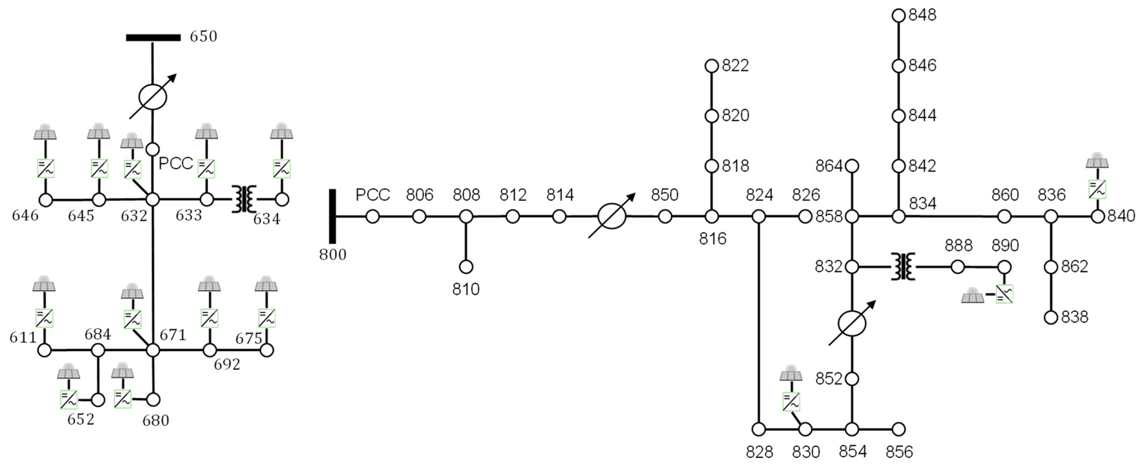
4. Case Study
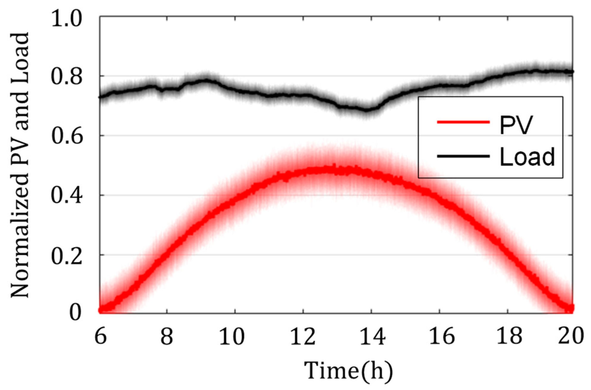
4.1. Simulation Data
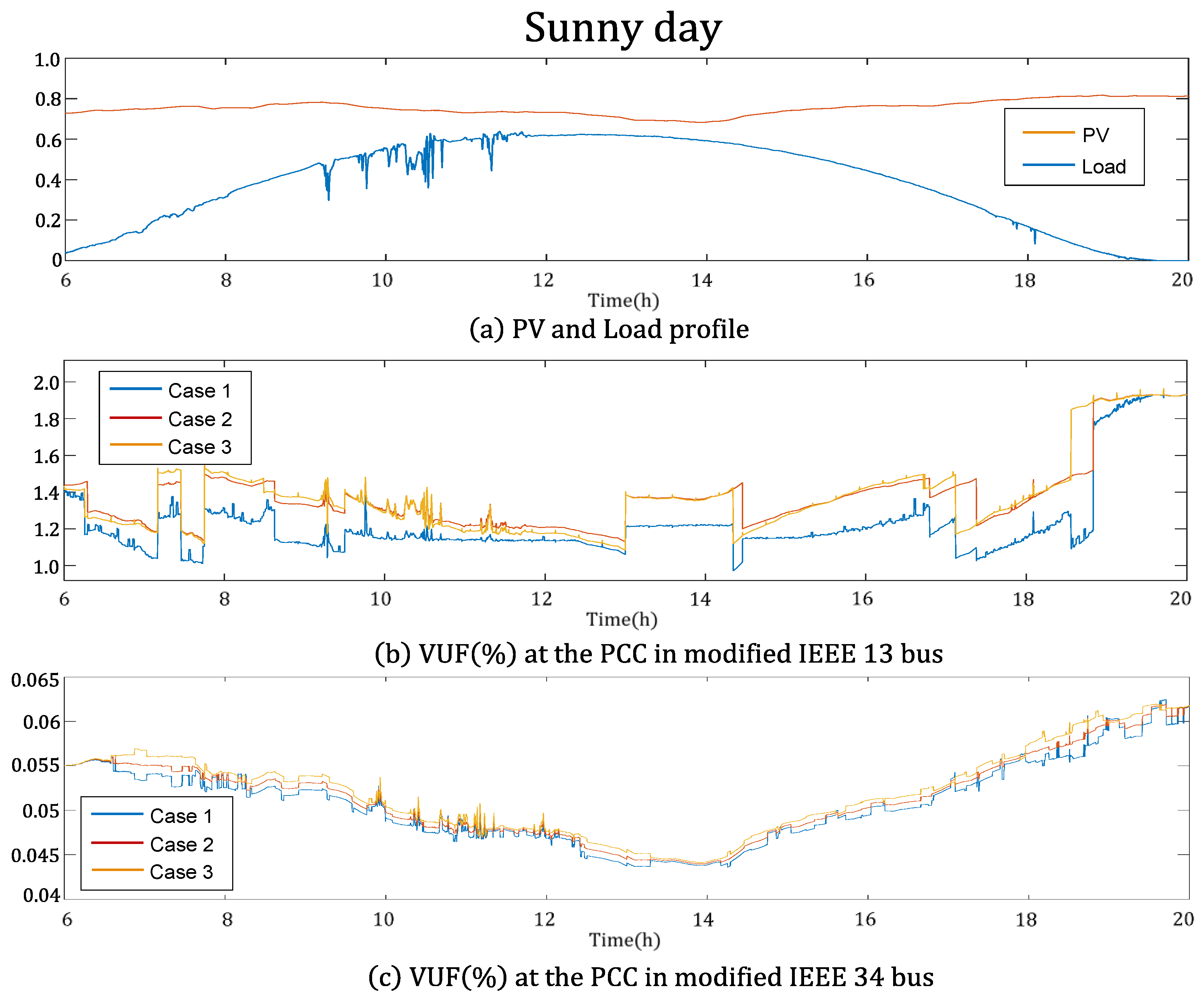
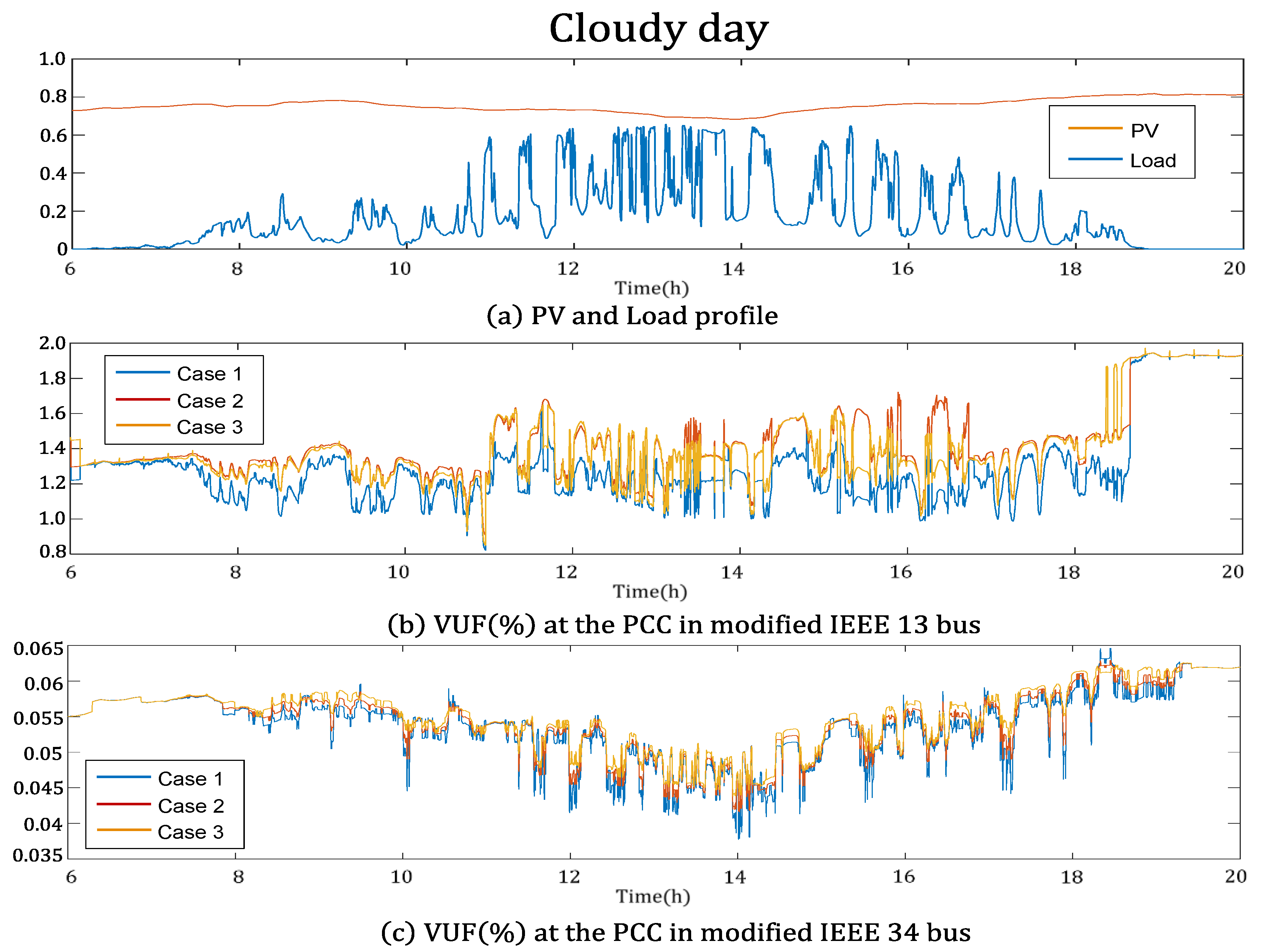
4.2. Comparison
- Case 1: inverters with volt–var curve controlled by the proposed method
- Case 2: inverters with volt–var curve with a fixed value
- Case 3: inverters with no reactive power compensation
4.3. Simulation Result
5. Conclusions and Future Work
Author Contributions
Funding
Conflicts of Interest
References
- Putrus, G.A.; Suwanapingkarl, P.; Johnston, D.; Bentley, E.C.; Narayana, M. Impact of electric vehicles on power distribution networks. In Proceedings of the 2009 IEEE Vehicle Power and Propulsion Conference, Dearborn, MI, USA, 7–10 September 2009; pp. 827–831. [Google Scholar]
- Balamurugan, K.; Srinivasan, D.; Reindl, T. Impact of distributed generation on power distribution system. Energy Procedia 2012, 25, 93–100. [Google Scholar] [CrossRef] [Green Version]
- Kersting, W.; Phillips, W. Phase frame analysis of the effects of voltage unbalance on induction machines. IEEE Trans. Ind. Appl. 1997, 33, 415–420. [Google Scholar] [CrossRef]
- Lee, C.Y. Effects of unbalanced voltage on the operation performance of a three-phase induction motor. IEEE Trans. Energy Convers. 1999, 14, 202–208. [Google Scholar]
- Jha, R.R.; Dubey, A.; Liu, C.C.; Schneider, K.P. Bi-level volt-var optimization to coordinate smart inverters with voltage control devices. IEEE Trans. Power Syst. 2019, 34, 1801–1813. [Google Scholar] [CrossRef] [Green Version]
- Nájera, J.; Mendonça, H.; de Castro, R.M.; Arribas, J.R. Strategies comparison for voltage unbalance mitigation in LV distribution networks using EV chargers. Electronics 2019, 8, 289. [Google Scholar] [CrossRef] [Green Version]
- Nejabatkhah, F.; Li, Y.W. Flexible unbalanced compensation of three-phase distribution system using single-phase distributed generation inverters. IEEE Trans. Smart Grid 2019, 10, 1845–1857. [Google Scholar] [CrossRef]
- Yao, M.; Hiskens, I.A.; Mathieu, J.L. Mitigating Voltage Unbalance Using Distributed Solar Photovoltaic Inverters. IEEE Trans. Power Syst. 2021, 36, 2642–2651. [Google Scholar]
- Schmidhuber, J. Deep learning in neural networks: An overview. Neural Netw. 2015, 61, 85–117. [Google Scholar] [CrossRef] [Green Version]
- Nguyen, T.T.; Nguyen, N.D.; Nahavandi, S. Deep reinforcement learning for multiagent systems: A review of challenges, solutions, and applications. IEEE Trans. Cybern. 2020, 50, 3826–3839. [Google Scholar] [CrossRef] [Green Version]
- Duan, J.; Yi, Z.; Shi, D.; Lin, C.; Lu, X.; Wang, Z. Reinforcement-learning-based optimal control of hybrid energy storage systems in hybrid AC–DC microgrids. IEEE Trans. Ind. Inform. 2019, 15, 5355–5364. [Google Scholar] [CrossRef]
- Duan, J.; Shi, D.; Diao, R.; Li, H.; Wang, Z.; Zhang, B.; Bian, D.; Yi, J. Deep-reinforcement-learning-based autonomous voltage control for power grid operations. IEEE Trans. Power Syst. 2019, 35, 814–817. [Google Scholar] [CrossRef]
- Wang, W.; Yu, N.; Shi, J.; Gao, Y. Volt-VAR control in power distribution systems with deep reinforcement learning. In Proceedings of the 2019 IEEE International Conference on Communications, Control and Computing Technologies for Smart Grids (SmartGridComm), Beijing, China, 21–23 October 2019; pp. 1–7. [Google Scholar]
- Huang, Q.; Huang, R.; Hao, W.; Tan, J.; Fan, R.; Huang, Z. Adaptive power system emergency control using deep reinforcement learning. IEEE Trans. Smart Grid 2020, 11, 1171–1182. [Google Scholar] [CrossRef] [Green Version]
- Zhang, Y.; Wang, X.; Wang, J.; Zhang, Y. Deep reinforcement learning based volt-var optimization in smart distribution systems. IEEE Trans. Smart Grid 2020, 12, 361–371. [Google Scholar] [CrossRef]
- Schulman, J.; Wolski, F.; Dhariwal, P.; Radford, A.; Klimov, O. Proximal policy optimization algorithms. arXiv 2017, arXiv:1707.06347. [Google Scholar]
- Fuller, A.; Fan, Z.; Day, C.; Barlow, C. Digital twin: Enabling technologies, challenges and open research. IEEE Access 2020, 8, 108952–108971. [Google Scholar] [CrossRef]
- Jouanne, A.V.; Banerjee, B. Assessment of voltage unbalance. IEEE Trans. Power Deliv. 2001, 16, 782–790. [Google Scholar] [CrossRef]
- Singh, A.K.; Singh, G.K.; Mitra, R. Some observations on definitions of voltage unbalance. In Proceedings of the 2007 39th North American Power Symposium, Las Cruces, NM, USA, 30 September–2 October 2007; pp. 473–479. [Google Scholar]
- Dzafic, I.; Donlagic, T.; Henselmeyer, S. Fortescue transformations for three-phase power flow analysis in distribution networks. In Proceedings of the 2012 IEEE Power and Energy Society General Meeting, San Diego, CA, USA, 22–26 July 2012; pp. 1–7. [Google Scholar]
- IEEE standard for interconnection and interoperability of distributed energy resources with associated electric power systems interfaces. In IEEE Std 1547–2018 (Revis. IEEE Std 1547–2003); IEEE: Piscataway Township, NJ, USA, 2018; pp. 1–138.
- Lipowski, A.; Lipowska, D. Roulette-wheel selection via stochastic acceptance. Phys. A Stat. Mech. Appl. 2012, 391, 2193–2196. [Google Scholar] [CrossRef] [Green Version]
- Korea Power Exchange. Available online: http://kpx.or.kr (accessed on 16 August 2021).
- Tostado-Véliz, M.; Kamel, S.; Jurado, F. Development and Comparison of Efficient Newton-Like Methods for Voltage Stability Assessment. Electr. Power Compon. Syst. 2020, 48, 1798–1813. [Google Scholar]
- Swief, R.A.; Hassan, N.M.; Abdelaziz, A.Y.; Kamh, M.Z. Multi-Regional Optimal Power Flow Using Marine Predators Algorithm Considering Load and Generation Variability. IEEE Access 2021, 9, 74600–74613. [Google Scholar] [CrossRef]
- Tostado-Véliz, M.; Kamel, S.; Jurado, F. Power flow solution of Ill-conditioned systems using current injection formulation: Analysis and a novel method. Int. J. Electr. Power Energy Syst. 2021, 127, 106669. [Google Scholar] [CrossRef]
- Dugan, R.C.; McDermott, T.E. An open source platform for collaborating on smart grid research. In Proceedings of the 2011 IEEE Power and Energy Society General Meeting, Detroit, MI, USA, 24–28 July 2011; pp. 1–7.
- PyTorch. Available online: http://pytorch.org (accessed on 19 August 2021).
- Bedawy, A.; Yorino, N.; Mahmoud, K.; Zoka, Y.; Sasaki, Y. Optimal Voltage Control Strategy for Voltage Regulators in Active Unbalanced Distribution Systems Using Multi-Agents. IEEE Trans. Power Syst. 2019, 35, 1023–1035. [Google Scholar] [CrossRef]


| Line-to-Line | Line-to-Neutral | ||||||||||||||
|---|---|---|---|---|---|---|---|---|---|---|---|---|---|---|---|
| Network | IEEE 13 Bus | IEEE 34 Bus | IEEE 13 Bus | ||||||||||||
| Location | 646 | 645 | 632 | 633 | 634 | 671 | 840 | 890 | 830 | 611 | 692 | 675 | 652 | 680 | |
| Capacity | (kVA) | 110 | 110 | 110 | 165 | 70 | 60 | 110 | 110 | 110 | 60 | 110 | 122 | 110 | 60 |
| (kW) | 100 | 100 | 100 | 150 | 60 | 50 | 100 | 100 | 100 | 50 | 100 | 110 | 100 | 50 | |
| Phase | 2 | 2 | 1 | 1 | 1 | 3 | 1, 2, 3 | 1, 2, 3 | 1, 2, 3 | 3 | 3 | 1 | 1 | 1 | |
| Network | Case 1 | Case 2 | Case 3 | ||
|---|---|---|---|---|---|
| Sunny day | IEEE 13 | 1.23 | 1.38 | 1.37 | |
| IEEE 34 | 0.05 | 0.0514 | 0.52 | ||
| Cloudy day | IEEE 13 | 1.29 | 1.40 | 1.42 | |
| IEEE 34 | 0.053 | 0.054 | 0.055 | ||
Publisher’s Note: MDPI stays neutral with regard to jurisdictional claims in published maps and institutional affiliations. |
© 2021 by the authors. Licensee MDPI, Basel, Switzerland. This article is an open access article distributed under the terms and conditions of the Creative Commons Attribution (CC BY) license (https://creativecommons.org/licenses/by/4.0/).
Share and Cite
Jung, Y.; Han, C.; Lee, D.; Song, S.; Jang, G. Adaptive Volt–Var Control in Smart PV Inverter for Mitigating Voltage Unbalance at PCC Using Multiagent Deep Reinforcement Learning. Appl. Sci. 2021, 11, 8979. https://0-doi-org.brum.beds.ac.uk/10.3390/app11198979
Jung Y, Han C, Lee D, Song S, Jang G. Adaptive Volt–Var Control in Smart PV Inverter for Mitigating Voltage Unbalance at PCC Using Multiagent Deep Reinforcement Learning. Applied Sciences. 2021; 11(19):8979. https://0-doi-org.brum.beds.ac.uk/10.3390/app11198979
Chicago/Turabian StyleJung, Yoongun, Changhee Han, Dongwon Lee, Sungyoon Song, and Gilsoo Jang. 2021. "Adaptive Volt–Var Control in Smart PV Inverter for Mitigating Voltage Unbalance at PCC Using Multiagent Deep Reinforcement Learning" Applied Sciences 11, no. 19: 8979. https://0-doi-org.brum.beds.ac.uk/10.3390/app11198979