A General Framework for Crankshaft Balancing and Counterweight Design

Abstract

In the automotive field, the requirements in terms of carbon emissions and improved efficiency are shifting the focus of designers towards reduced engine size. As a result, the dynamic balancing of an engine with strict limitations on the number of cylinders, the weight and the available space becomes a challenging task. The present contribution aims at providing the designer with a tool capable of selecting fundamental parameters needed to correctly balance an internal combustion engine, including the masses and geometry of the elements to be added directly onto the crankshaft and onto the balancing shafts. The relevant elements that distinguish the tool from others already proposed are two. The first is the comprehensive matrix formulation which makes the tool fit for a wide variety of engine configurations. The second is an optimisation procedure that selects not only the position of the mass and centre of gravity of the counterweight but also its complete geometric configuration, thus instantaneously identifying the overall dimensions and weight of the crankshaft.

1. Introduction

The modern automotive market requires a continuous reduction of carbon emissions and fuel consumption and an ever increasing engine efficiency [1,2]. These goals can be achieved by the use of a support electric motor for functions such as the Start/Stop or real hybrid engines. The engine compartment must then accommodate these new components; therefore, engine dimensions must be as small as possible, especially in the case of small/medium size cars. Furthermore, engine downsizing is recognised, in itself, as an effective method to reduce consumption and increase efficiency [3,4] and many manufacturers are reducing engine displacement and the number of cylinders.

From a design point of view, the combination of a reduced number of cylinders with weight and space limitations makes the task of balancing the crankshaft more difficult. Crankshaft unbalance translates into high vibrations that are transmitted to the entire car, thus compromising the user comfort level [5]. Crankshaft balancing is typically performed in two subsequent phases. The first is during the early design, where the configuration of the masses to be added to the crankshaft and to the additional balance shafts are defined [6]. The second involves the measurement of the residual unbalance [7] in machined crankshafts and the subsequent correction on a sample-to-sample basis [8,9]. The contribution of the present work fits precisely into the first step of the balancing process and was developed to aid the designer in choosing, since the early stages, the weight and the configuration of masses to be added to the crankshaft and, when present, to the balance shafts.

It must be noted that the goal of the present tool is to perform a “global” balancing of the system, in order to find the optimal counterweight configuration. The introduction of the counterweights produces a change in the reaction forces and in the loading diagram of each journal bearing. Therefore, once the counterweight configuration has been defined, it is of paramount importance to evaluate how this change may influence the design of the journal bearings themselves [10,11,12,13], an aspect which is, however, beyond the scope of the present work.

The proposed tool, equipped with a Graphical User Interface, is based on a comprehensive formulation which allows the user to analyse a wide range of scenarios, i.e., crankshafts with any number of cylinders and counterweights, in-line and V configurations alike. The proposed framework needs as input only the main geometrical dimensions and key operating conditions (e.g., piston firing order), and offers, as outputs, the rotating vectors diagrams and the counterweights mass and configuration necessary to balance the centrifugal forces and the first and second order reciprocating forces and the respective moments.

The basic concepts and formulation adopted by the tool are presented in Section 2.

The matrix formulation adopted to express the balancing equations is presented and discussed to highlight its versatility in Section 3. Section 4 is devoted to the parametrization of the counterweight shape and its subsequent optimisation, a problem which is either tackled through an iterative procedure requiring a lengthy direct involvement from the designer [14] or through the use of computationally intensive CAD-based genetic algorithms [15].

The numerical tool, whose user interface is described in Section 5, is then used in Section 6 to investigate different scenarios, demonstrating its effectiveness in exploring the counterweights’ minimum weight-minimum dimension trade-off.

2. Methodology

Balancing Concepts

The creation of the tool starts from the definition of a suitable model of the crankshaft with the relative forces that need balancing. A generic crankshaft can be divided into multiple elementary elements, called cranks, identified and oriented based on the firing order of the engine. Each crank is made of three parts:

• two main journals, which are supported by the engine block;
• one crank-pin, on which the big-eye of the connecting rod is placed;
• two crank webs, which connect the main journals and the crank-pin.

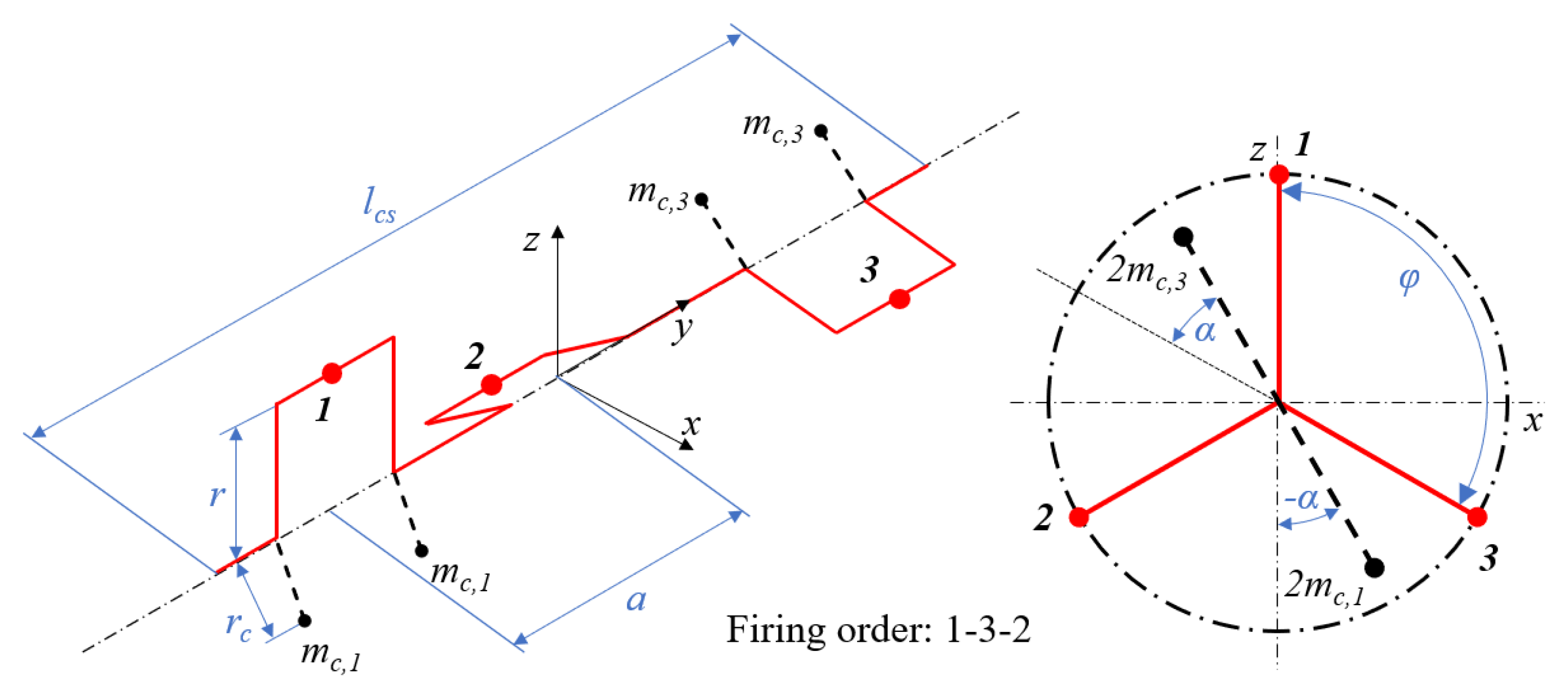
These components are modelled as rigid beams, made of the same material. Such model can be seen in Figure 1. In this figure the dimensions relevant to the balancing process can be identified, alongside the reference system adopted throughout the analysis.

It is possible to identify three forces in need of balancing in the engine:

• Centrifugal force, $F_{\omega }=m_{rot}{\omega }^{2}r$;
• Primary reciprocating force, $F_a^{{}^{\prime }}=-m_{alt}{\omega }^{2}r\left(cos\theta \right)$;
• Secondary reciprocating force, $F_a^{{}^{″}}=-m_{alt}{\omega }^{2}r\left(\mathsf{\Lambda }cos2\theta \right)$

where $m_{rot}$ is the rotational mass of the crank mechanism (including crank webs, crankpin and conrod’s big-eye), $m_{alt}$ is the crank mechanism reciprocating mass (including piston, wristpin, piston rings and conrod’s small-eye), $\omega$ is the crankshaft rotational speed, $\theta$ is the crank-angle with respect to the z-axis and $\mathsf{\Lambda }$ is the elongation ratio, equal to the ratio between the crank radius r and the conrod length. The minus sign for the reciprocating forces is representative of the fact that the inertia forces have opposite direction with respect to the direction of motion of the pistons. The centrifugal force $F_{\omega }$ has constant magnitude but its direction continuously changes coherently with the crankshaft rotation angle, meanwhile the reciprocating forces $F_a^{{}^{\prime }},F_a^{{}^{″}}$ are always aligned with their respective cylinder axis and the magnitude changes continuously, with the secondary one having double the frequency of the primary reciprocating force. In any case, the behaviour is clearly oscillating; therefore, these forces, and the possible moments they may form, can generate deformations of the crankshaft which must be minimised.

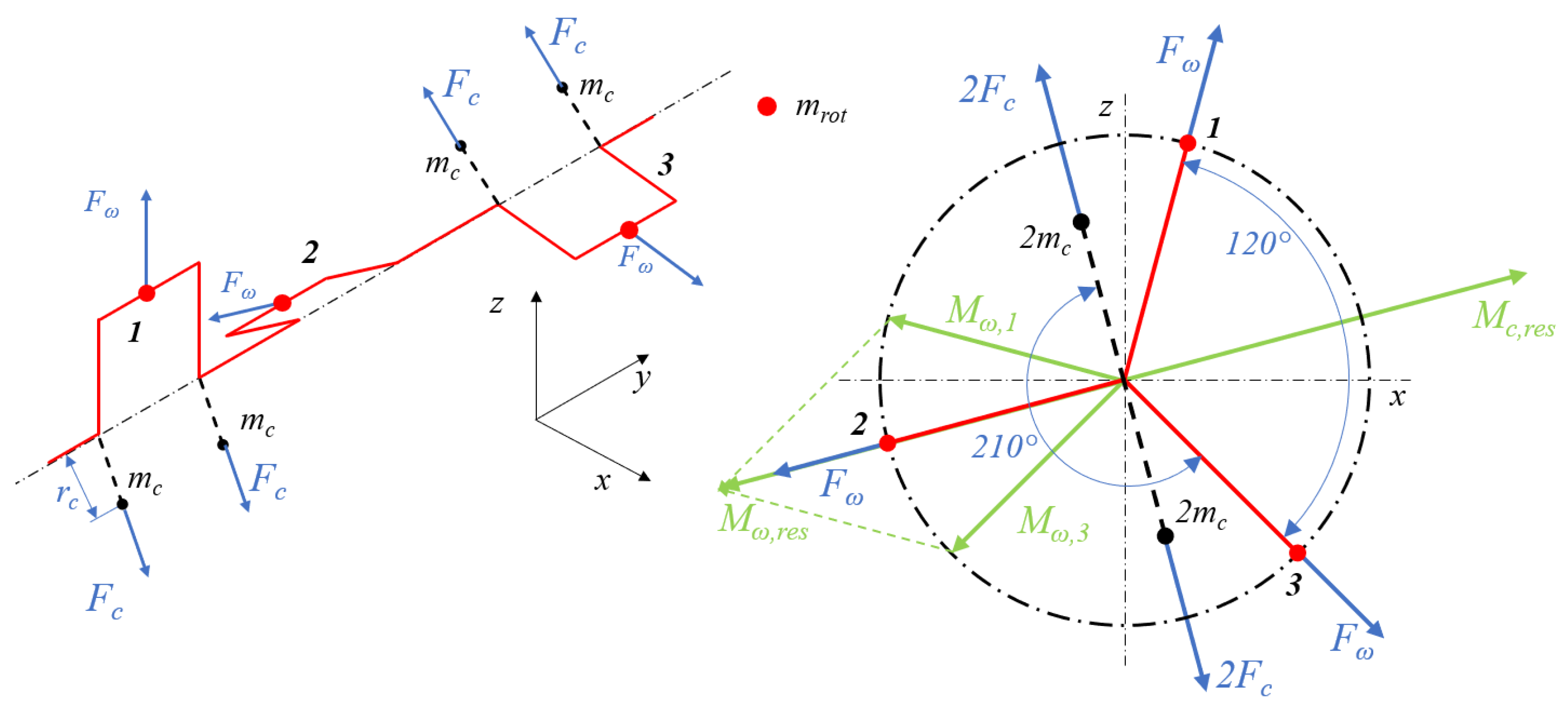
The balancing of the forces can be performed by adding to the engine properly sized masses, called counterweights. These masses will rotate during the operation of the engine, generating centrifugal forces that counter those of the crankshaft. It is possible to place the counterweights through two main methods: either directly on the crankshaft or on additional components called balancing shafts. For what concerns the centrifugal force balancing, it depends on the rotational masses of the crankshaft $m_{rot}$, composed of the masses of the crank-pin, the two crank-webs and the big-eye of the connecting rod, and, due to its constant magnitude, it is sufficient to place the counterweights on the crankshaft, as shown in Figure 2, where the following quantities can be identified: $F_c$ are the centrifugal forces generated by the counterweights $m_c$, $M_{\omega ,1}$ and $M_{\omega ,3}$ are the moments by the cranks (1 and 3 respectively), $M_{\omega ,res}$ is the resultant of the previously defined moments and $M_{c,res}$ is the moment generated by the counterweight centrifugal forces. The numerical subscripts refer to the cylinder number and in the following discussion are removed for simplicity, since the elements share the same magnitude (e.g., $m_{c,1}$ and $m_{c,3}$ will be defined as $m_c$).

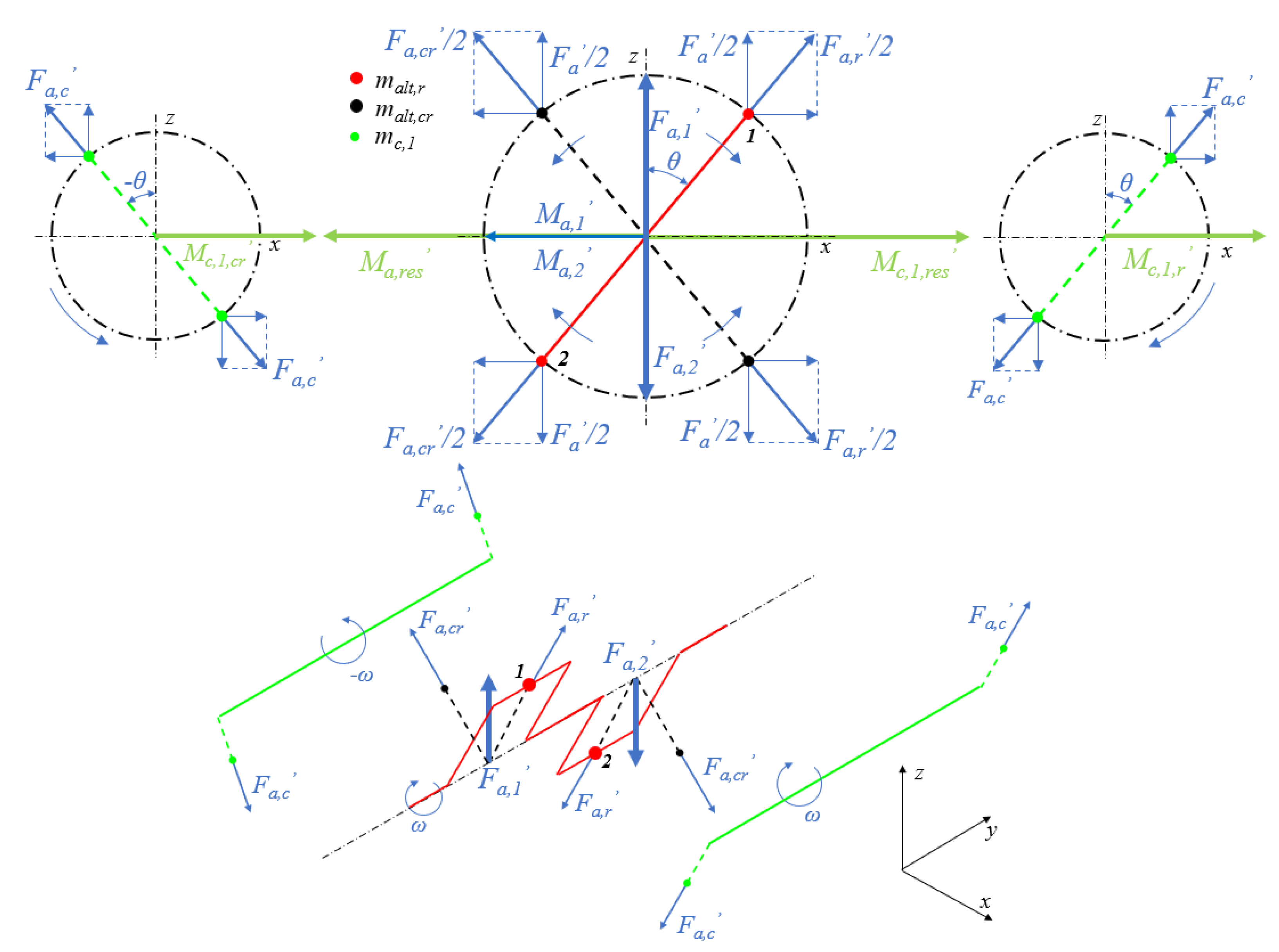
The reciprocating forces, instead, due to their direction always aligned with the cylinders axis, cannot be treated as the centrifugal force. The most commonly adopted model converts the force into two “equivalent” contributions: considering the radius of these contributions equal to the crank radius, the ones for the primary reciprocating forces are equal to $\frac{m_{alt}}{2}$, while the ones for the secondary reciprocating forces are equal to $\frac{m_{alt}\mathsf{\Lambda }}{8}$. One of these fictitious masses rotates, while the other one counter-rotates, along with the trajectory of the centre of mass of the crank-pin. These masses have the same speed as the crankshaft when considering the primary reciprocating force; meanwhile, the masses for the secondary reciprocating force has double the speed of the crankshaft. The sum of the z-components of the centrifugal forces that these masses generate is then equal to the corresponding actual reciprocating force. With such conversion, it is possible to balance each individual force through the addition of the counterweights. For the primary reciprocating force, the main method makes use of two balancing shafts, one for the rotating and one for the counter-rotating masses, as shown in Figure 3, where the following quantities can be identified: $m_{alt,r}$ and $m_{alt,cr}$, which are respectively the rotating and counter-rotating fictitious masses, both equal to $m_{alt}/2$, $m_{c,1}$, the counterweights mass for the primary reciprocating force, $F_{a,r}^{{}^{\prime }}$ and $F_{a,cr}^{{}^{\prime }}$, which are the centrifugal forces for respectively the rotating and counter-rotating fictitious masses, $F_{a,1}^{{}^{\prime }}$ and $F_{a,2}^{{}^{\prime }}$, which are the primary reciprocating force for each cylinder (1 and 2, respectively) and each one equal to $F_a^{{}^{\prime }}$, $M_{a,1}^{{}^{\prime }}$ and $M_{a,2}^{{}^{\prime }}$, the moments generated by the previously defined forces, $F_{a,c}^{{}^{\prime }}$, which is the centrifugal force generated by the counterweights, $M_{c,1,r}^{{}^{\prime }}$ and $M_{a,1,cr}^{{}^{\prime }}$, the moments generated by the rotating and counter-rotating shafts, and $M_{a,res}^{{}^{\prime }}$ and $M_{c,1,res}^{{}^{\prime }}$, the resultants of, respectively, the crankshaft and the balancing shafts moments.

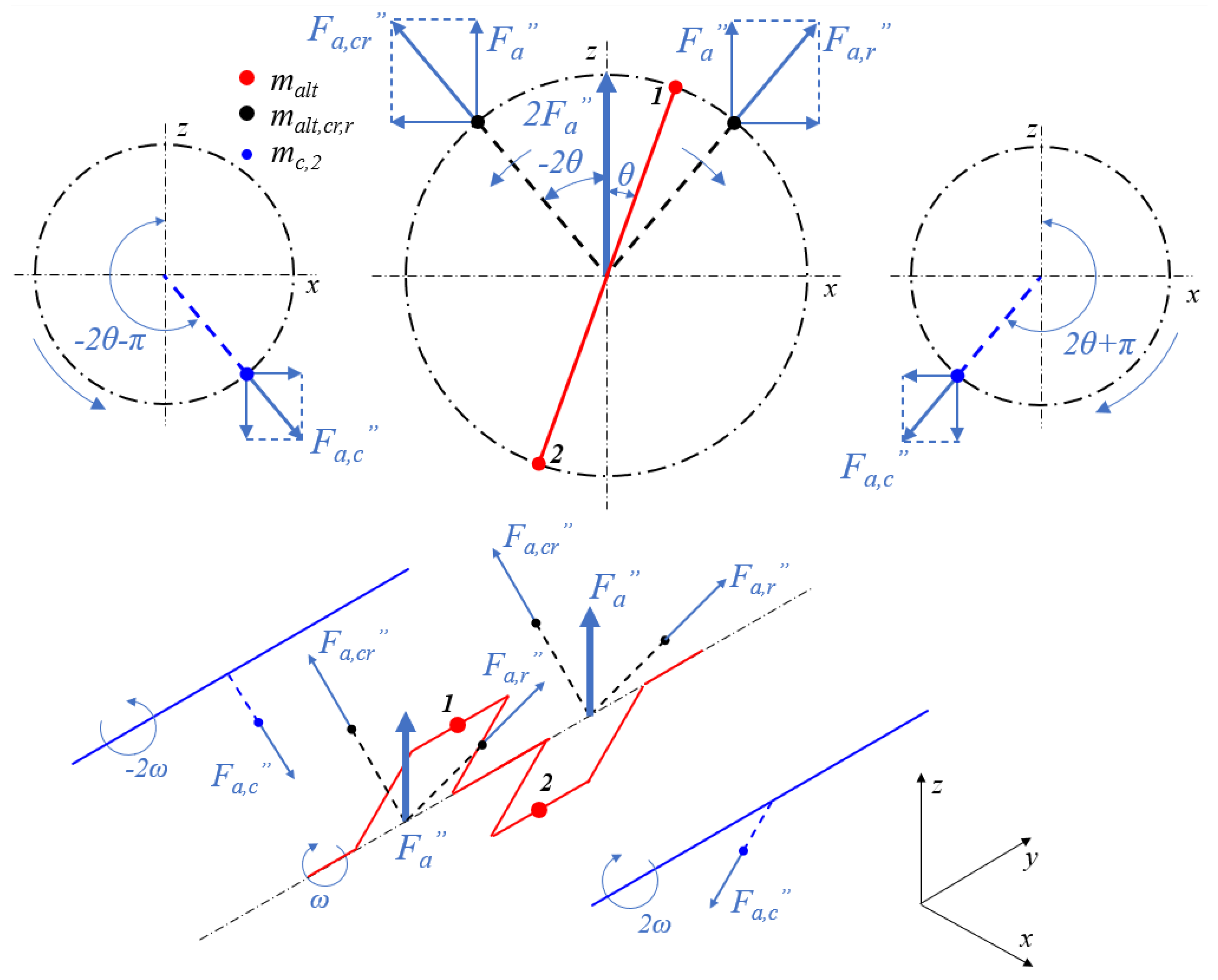
A similar balancing method can be used for the secondary reciprocating forces. In this case the balancing shaft will rotate at double the speed of the crankshaft, as it is reported in Figure 4, where the following quantities can be identified: $m_{alt,cr,r}$, which represents both the rotating and counter-rotating fictitious masses, which, in this view, in this specific configuration, are overlapping, and are both equal to $m_{alt}/2$, $m_{c,2}$, the counterweights mass for the secondary reciprocating force, $F_{a,r}^{{}^{″}}$ and $F_{a,cr}^{{}^{″}}$, which are the centrifugal forces for respectively the rotating and counter-rotating fictitious masses, $F_{a,c}^{{}^{″}}$, which is the centrifugal force generated by the counterweights.

3. Tool Design

Once the balancing requirements in terms of dynamic equilibrium of the crankshaft are defined, it is possible to proceed with the creation of the code in charge of computing the masses and orientation of the balancing components required by the engine configuration defined by the inputs provided by the user. Unlike other existing codes, the one proposed here can be easily adapted to a wide range of crankshaft configurations. This flexibility is achieved thanks to a modular matrix-based formulation, which will be extensively presented in the following paragraphs. It must be noted that the balancing performed by the code is a "global" one, so it does not consider the specific local forces on each individual bearing and the forces that the addition of counterweights could generate on the crankshaft, for which much more extensive analysis should be performed.

The first section of the code is designed to create the matrices useful to define the geometry of the crankshaft with its counterweights. The inputs used in the definition of such matrices are the following:

• Number of cranks, $N_{cr}$;
• Vector of the firing order, $F{O}_{1,N_{cr}}$;
• Crank angle of the first crank, $\theta$;
• Distance between the mid-points of two consecutive cranks, a;
• Phase between two cranks (based on firing order), $\varphi$;
• Angle between counterweight and crankpin symmetrical opposite, $\alpha$;
• Vector for definition of counterweight configuration, $Y_{cw}$.

The creation of the crankshaft matrix $CS$ starts by defining the reference system of the crankshaft: it is positioned at the mid-length of the component, with the y-axis aligned with the rotational axis of the crankshaft itself. Such reference system and the inputs previously defined are reported in Figure 1.

The crankshaft is thus defined by obtaining the position and orientation of each crank with respect to the reference system. The reference point taken for each crank corresponds to the mid-length of the crank journal, which also coincides with the centre point of the big eye of the con-rod. If we define $N_{fo}=FO\left(i\right)$ with $1\le i\le N_{cr}\in \mathbb{N}$, the formulation of $CS$, is as follows:

$$CS(1,N_{fo})=\left[\sin (\theta +(i-1)\varphi )\right]$$

(1)

$$CS(2,N_{fo})=\left[(N_{fo}-1)a-\frac{(N_{cr}-1)}{2}a\right]$$

(2)

$$CS(3,N_{fo})=\left[\cos (\theta +(i-1)\varphi )\right]$$

(3)

From these equations we can see that the geometry matrix for the crankshaft will be a $3-by-N_{cr}$ matrix, with the first, second and third row, i.e., Equations (1)–(3), the x, y and z components of the crankpin centre position respectively. Meanwhile, each column represents the set of components for each crank of the crankshaft. The following equation is an example of matrix for the crankshaft geometry, shown in Figure 1:

$$CS=\left(\begin{array}{ccc}0& sin\left(\frac{4}{3}\pi \right)& sin\left(\frac{2}{3}\pi \right)\\ -a& 0& a\\ 1& cos\left(\frac{4}{3}\pi \right)& cos\left(\frac{2}{3}\pi \right)\end{array}\right)$$

(4)

The matrix of the crankshaft counterweights $CW$ is then created. The reference system and method is the same as those followed for $CS$: for each counterweight, a column representing the three components of the counterweight position will be defined. Since not all crankswebs will be equipped with a counterweight, a vector of ones and zeros, termed $Y_{cw}$, is used to signal the presence of a counterweight in a given position.

$$Y_{cw}=\left[110011\right]$$

(5)

The example in Equation (5) is the vector for the 3 cylinder in-line engine with four counterweight presented in Figure 1. It should be noted that, since we have two crankwebs for each crank, the dimension of $Y_{cw}$ is twice the number of cranks, with ones that indicate the presence and zeros the absence of a counterweight. So, if we define $N_{fo}=FO\left(i\right)$ with $1\le i\le N_{cr}\in \mathbb{N}$ and, $\forall i$$N_{cw}=Y_{cw}\left(j\right)$ with $j=2i-1$∧$j=2i$, we can create the matrix as follows:

$$CW(1,j)=\left[\sin (\theta +(i-1)\varphi +\alpha )\right](-N_{cw})$$

(6)

$$\left\{\begin{array}{c}CW(2,j)=\left[\left[(N_{fo}-1)a-\frac{(N_{cr}-1)}{2}a\right]-a/4\right]\left(N_{cw}\right)forj=2i-1\hfill \\ CW(2,j)=\left[\left[(N_{fo}-1)a-\frac{(N_{cr}-1)}{2}a\right]+a/4\right]\left(N_{cw}\right)forj=2i\hfill \end{array}\right.$$

(7)

$$CW(3,j)=\left[\cos (\theta +(i-1)\varphi +\alpha )\right](-N_{cw})$$

(8)

where $\alpha$ is negative when $N_{fo}\le N_{cr}/2$ and is positive when $N_{fo}\ge N_{cr}/2$. The matrix for the counterweight configuration of the 3 cylinder engine previously defined becomes as follows:

$$CW=\left(\begin{array}{cccccc}-sin\left(-\alpha \right)& -sin\left(-\alpha \right)& 0& 0& -sin\left(\frac{2}{3}\pi +\alpha \right)& -sin\left(\frac{2}{3}\pi +\alpha \right)\\ -a-a/4& -a+a/4& 0& 0& a-a/4& a+a/4\\ -cos\left(-\alpha \right)& -cos\left(-\alpha \right)& 0& 0& -cos\left(\frac{2}{3}\pi +\alpha \right)& -cos\left(\frac{2}{3}\pi +\alpha \right)\end{array}\right)$$

(9)

The matrix $CW$ has dimensions 3-by-6, with the three x-y-z components as rows and as many columns as the number of crank webs, with the two central columns equal to zero because the counterweights are not applied in those positions.

3.1. Centrifugal Forces Balancing

Once the matrices for the crankshaft and relative counterweights have been created, the next step that the code undertakes is the computation of the mass of each counterweight, which is assumed the same for each counterweight. This assumption seems reasonable since, given the similarity among cylinders belonging to the same engine and the symmetry of the crankshaft, a uniform distribution of the counterweight masses is the best option to avoid additional unbalance. The method used for the calculation starts from the equations of equilibrium, both of forces and moments, and expresses them using the matrices previously defined.

The equations of equilibrium that we can define are four, two for the forces and two for the moments:

$$\left\{\begin{array}{c}\sum _{i=1}^{N_{cr}}{m}_{rot}{\omega }^{2}rCS(1,i)=\sum _{j=1}^{2N_{cr}}{m}_c{\omega }^2{r}_{c}CW(1,j)\hfill \\ \sum _{i=1}^{N_{cr}}{m}_{rot}{\omega }^{2}rCS(3,i)=\sum _{j=1}^{2N_{cr}}{m}_c{\omega }^2{r}_{c}CW(3,j)\hfill \\ \sum _{i=1}^{N_{cr}}{m}_{rot}{\omega }^{2}rCS(1,i)CS(2,i)=\sum _{j=1}^{2N_{cr}}{m}_c{\omega }^2{r}_{c}CW(1,j)CW(2,j)\hfill \\ \sum _{i=1}^{N_{cr}}{m}_{rot}{\omega }^{2}rCS(3,i)CS(2,i)=\sum _{j=1}^{2N_{cr}}{m}_c{\omega }^2{r}_{c}CW(3,j)CW(2,j)\hfill \end{array}\right.$$

(10)

where $r_c$ is the radius of the centre of gravity of the crankshaft counterweights. The first two equations are the equilibrium of the forces, the first being for the x-component and the second for the z-component; the last two equations, instead, are for the moments, in this case around the x and z axis. We can also see that the first term of each equation represents the resultant of forces and moments generated by the cranks, while the second term is for the counterweights resultants. From these equations it is possible to derive an equation to obtain the needed unknown quantities. For instance, fixing $r_c$ to a given value, one can derive $m_c$:

$$\left\{\begin{array}{c}{m}_c=\frac{{\sum }_{i=1}^{N_{cr}}{m}_{rot}rCS(1,i)}{{\sum }_{j=1}^{2N_{cr}}{r}_{c}CW(1,j)}\hfill \\ m_c=\frac{{\sum }_{i=1}^{N_{cr}}{m}_{rot}rCS(3,i)}{{\sum }_{j=1}^{2N_{cr}}{r}_{c}CW(3,j)}\hfill \\ m_c=\frac{{\sum }_{i=1}^{N_{cr}}{m}_{rot}rCS(1,i)CS(2,i)}{{\sum }_{j=1}^{2N_{cr}}{r}_{c}CW(1,j)CW(2,j)}\hfill \\ m_c=\frac{{\sum }_{i=1}^{N_{cr}}{m}_{rot}rCS(3,i)CS(2,i)}{{\sum }_{j=1}^{2N_{cr}}{r}_{c}CW(3,j)CW(2,j)}\hfill \end{array}\right.$$

(11)

It must be noted that not all of these equations are needed to find the counterweight mass, but just one is necessary. However, it is important to consider them all, initially, because some crankshaft configurations have a null resultant of the forces and others a null resultant of the moments. Therefore, the equation that must be used from the set in Equation (11) is the one that has a numerator different from zero.

A particular situation that can be encountered is when all of the resultants previously defined are null. This means that both in terms of forces and in terms of moments around the mid-point of the crankshaft, the engine is balanced. However, this usually happens in relatively long crankshafts, like 4 and 6 cylinder in-line engines, in which each half-crankshaft can create unbalancing moments. In this case, the code will automatically recognise the situation and compute the masses of the counterweights based on the same equations but considering only half of the crankshaft: this is managed by having the sums in Equation (10) starting from one and reaching $N_{cr}/2$ and $N_{cr}$ for the crank and counterweights term, respectively.

3.2. Primary Reciprocating Forces Balancing

The balancing of the primary reciprocating force needs, along with some of the data already used for the centrifugal balancing, the following additional inputs:

• The total length of the primary balancing shafts (which corresponds to the distance between the outer counterweights of the shafts), $l_{sh,1}$;
• The radius of the centre of gravity of the primary counterweights, $r_{c,1}$.

Such inputs can be visualised in Figure 7. For the perfect balancing of the primary reciprocating forces, as described in Section 2, two balancing shafts are needed. Each of the shafts must balance the forces and moments that the reciprocating components generate. Therefore, the first step is to create the geometry matrix for the shafts. Two main cases can originate in terms of reciprocating forces: one with the force resultant different from zero and one with the moment resultant different from zero. Based on the case, the counterweights can be one per shaft, in their mid-position, or two at the extremities. The matrices for the rotating and counter-rotating shafts can be defined as follows:

$$C{W}_{1,r}(1,k)=CW(1,i)C{W}_{1,cr}(1,k)=-CW(1,i)$$

(12)

$$C{W}_{1,r}\left(2\right)=[-l_{sh,1}{l}_{sh,1}]C{W}_{1,cr}\left(2\right)=[-l_{sh,1}{l}_{sh,1}]$$

(13)

$$C{W}_{1,r}(3,k)=CW(3,i)C{W}_{1,cr}(3,k)=-CW(3,i)$$

(14)

where for $k=1$, $i=1$ and for $k=2$, $i=2N_{cr}$. The matrices found with these equations are the ones relative to the case when the moment resultant is different from zero. When the other case is encountered the matrix becomes a vertical array per shaft with the same x and z components for $k=1$ and the y-component equal to zero. The single mass on each shaft can be also divided into multiple masses, if the symmetry around the mid-point of the shafts is maintained.

With the matrices defined, it is then possible to formulate the equations for the computation of the masses that must be applied to the balancing shafts, $m_{c1}$:

$$\left\{\begin{array}{c}\sum _{i=1}^{N_{cr}}{m}_{alt}{\omega }^{2}rCS(3,i)=\sum _{j=1}^{N_{cw,1}}{m}_{c,1}{\omega }^2{r}_{c,1}C{W}_{1,r}(3,j)+\hfill \\ +\sum _{j=1}^{N_{cw,1}}{m}_{c,1}{\omega }^2{r}_{c,1}C{W}_{1,cr}(3,j)\hfill \\ \\ \sum _{i=1}^{N_{cr}}{m}_{alt}{\omega }^{2}rCS(3,i)CS(2,i)=\sum _{j=1}^{N_{cw,1}}{m}_{c,1}{\omega }^2{r}_{c,1}C{W}_{1,r}(3,j)C{W}_{1,r}(2,j)+\hfill \\ +\sum _{j=1}^{N_{cw,1}}{m}_{c,1}{\omega }^2{r}_{c,1}C{W}_{1,cr}(3,j)C{W}_{1,cr}(2,j)\hfill \end{array}\right.$$

(15)

where $N_{cw,1}$ is the number of counterweights per shaft and $m_{alt}$ is the reciprocating mass of one cylinder. We can notice that the equations for the equilibrium are two: one for the equilibrium of the forces and one for the moments. Unlike the centrifugal forces, the primary reciprocating forces do not need the definition of the two components, since they are always coincident with the cylinder axis. The first term in the equations represents the sum of the forces/moments generated by the crankshaft, meanwhile the second term is given by the sum of the total forces/moments generated by the masses $m_{c,1}$ on the rotating and counter-rotating shafts. From Equation (15), we can then derive the following ones:

$$\left\{\begin{array}{c}{m}_{c,1}=\frac{{\sum }_{i=1}^{N_{cr}}{m}_{alt}rCS(3,i)}{{\sum }_{j=1}^{N_{cw,1}}{r}_{c,1}C{W}_{1,r}(3,j)+{\sum }_{j=1}^{N_{cw,1}}{r}_{c,1}C{W}_{1,cr}(3,j)}\hfill \\ \\ m_{c,1}=\frac{{\sum }_{i=1}^{N_{cr}}{m}_{alt}rCS(3,i)CS(2,i)}{{\sum }_{j=1}^{N_{cw,1}}{r}_{c,1}C{W}_{1,r}(3,j)C{W}_{1,r}(2,j)+{\sum }_{j=1}^{N_{cw,1}}{r}_{c,1}C{W}_{1,cr}(3,j)C{W}_{1,cr}(2,j)}\hfill \end{array}\right.$$

(16)

Similarly to the equations for the centrifugal counterweights, it is not necessary to use both equations of Equation (16) to compute the mass. Instead, the equation with a non-zero numerator must be used, since, as described earlier, the cases that are most likely encountered are those with the force resultant different from zero and one with the moment resultant different from zero. This means that the code would use, respectively, the first and second equation.

In order to reduce the complexity of the engine, it is possible to choose to eliminate the rotating shaft and substituting it with an additional mass that is included to each crankshaft counterweight. Since the forces and moment resultants must be the same, it is just needed to perform a conversion based on the radii of the counterweights and their number, as such:

$$m_{c,1,cs}=\frac{m_{c,1}r{N}_{cw,1}}{r_{c,1}{N}_{cw}}$$

(17)

where $N_{cw}$ is the number of crankshaft counterweights. It must be noted that such configuration may generate an additional moment around the y-axis in case of unbalanced primary reciprocating forces. This is due to the distance between the crankshaft and the counterrotating shaft and the absence of the rotating shaft, which would provide the balance around said axis.

3.3. Secondary Reciprocating Forces Balancing

The balancing of the secondary reciprocating forces needs the following additional inputs:

• The total length of the secondary balancing shafts (which corresponds to the distance between the outer counterweights of the shafts), $l_{sh,2}$;
• The radius of the centre of gravity of the secondary counterweights, $r_{c,2}$.

Such inputs can be visualised in Figure 7. Unlike the centrifugal and primary reciprocating forces, where the geometry matrix of the counterweights can be directly derived from the crankshaft matrix, the geometry matrices for the counterweights of the secondary reciprocating forces are more complex to derive, since they rotate at double the speed of the crankshaft and the relative position to the other components can change drastically between different crankshaft configurations.

The method exploits the fact that the reciprocating forces are always aligned with the cylinder axis and, therefore, the counterweights are parallel to the cylinder axis when the resultant force/moment of the cranks is maximum: in fact, only when the counterweights are parallel to the z-axis they generate the maximum vertical force and maximum moment around the x-axis. So, the code will proceed to compute the maximum values of resultant force and moments generated by the crankshaft, through the following equations:

$$\left\{\begin{array}{c}{F}_{a,2,res}=\sum _{i=1}^{N_{cr}}{m}_{alt}\mathsf{\Lambda }{\omega }^{2}rcos(2arccos\left(CS(3,i)\right))\hfill \\ M_{a,2,res}=\sum _{i=1}^{N_{cr}}{m}_{alt}\mathsf{\Lambda }{\omega }^{2}rcos(2arccos\left(CS(3,i)\right))CS(2,i)\hfill \end{array}\right.$$

(18)

When the maximum value of the force and moment is obtained, the corresponding crank angle of the first crank is saved and defined as $ϵ$. With this premise, it is then possible to create the geometry matrices for the counterweights of both shafts:

$$C{W}_{2,r}(1,k)=\sin (2\theta -2ϵ+\pi (k-1))C{W}_{2,cr}(1,k)=-C{W}_{2,r}(1,k)$$

(19)

$$C{W}_{2,r}(2,k)=\frac{-l_{sh,2}}{2}+l_{sh,2}(k-1)C{W}_{2,cr}(2,k)=\frac{-l_{sh,2}}{2}+l_{sh,2}(k-1)$$

(20)

$$C{W}_{2,r}(3,k)=\sin (2\theta -2ϵ+\pi (j-1))C{W}_{2,cr}(3,k)=C{W}_{2,r}(3,k)$$

(21)

where $k=1$ ∧ $k=2$, and $j=k$. Similarly to the primary reciprocating forces, the matrices found with these equations are those relative to the case where the moment resultant is different from zero. When the other case is encountered the matrix becomes a vertical array per shaft with the same x and z components for $k=1$, with $j=2$, and the y-component equal to zero. The single mass on each shaft can be also divided into multiple masses, if the symmetry around the mid-point of the shafts is maintained.

Once the matrices have been found, the equations of equilibrium are used to find the masses to apply to the counterweights, $m_{c,2}$. Effectively, the method follows the same exact pattern as for the primary reciprocating forces: -4.6cm 0cm

$$\left\{\begin{array}{c}\sum _{i=1}^{N_{cr}}{m}_{alt}\mathsf{\Lambda }{\omega }^{2}rcos(2arccos(3,i))=\sum _{j=1}^{N_{cw,2}}{m}_{c,2}4{\omega }^2{r}_{c,2}C{W}_{2,r}(3,j)+\hfill \\ +\sum _{j=1}^{N_{cw,2}}{m}_{c,2}4{\omega }^2{r}_{c,1}C{W}_{2,cr}(3,j)\hfill \\ \\ \sum _{i=1}^{N_{cr}}{m}_{alt}\mathsf{\Lambda }{\omega }^{2}rcos(2arccos(3,i))CS(2,i)=\sum _{j=1}^{N_{cw,2}}{m}_{c,2}{\omega }^2{r}_{c,2}C{W}_{2,r}(3,j)C{W}_{2,r}(2,j)+\hfill \\ +\sum _{j=1}^{N_{cw,2}}{m}_{c,2}{\omega }^2{r}_{c,2}C{W}_{2,cr}(3,j)C{W}_{2,cr}(2,j)\hfill \end{array}\right.$$

(22)

From these equations, we can then derive:

$$\left\{\begin{array}{c}{m}_{c,2}=\frac{{\sum }_{i=1}^{N_{cr}}{m}_{alt}\mathsf{\Lambda }rcos(2arccos(3,i))}{{\sum }_{j=1}^{N_{cw,2}}4r_{c,2}C{W}_{2,r}(3,j)+{\sum }_{j=1}^{N_{cw,2}}4r_{c,2}C{W}_{2,cr}(3,j)}\hfill \\ m_{c,2}=\frac{{\sum }_{i=1}^{N_{cr}}{m}_{alt}\mathsf{\Lambda }rcos(2arccos(3,i))CS(2,i)}{{\sum }_{j=1}^{N_{cw,2}}4r_{c,2}C{W}_{2,r}(3,j)C{W}_{2,r}(2,j)+{\sum }_{j=1}^{N_{cw,2}}4r_{c,2}C{W}_{2,cr}(3,j)C{W}_{2,cr}(2,j)}\hfill \end{array}\right.$$

(23)

Just like the primary reciprocating forces, only one equation from the set in Equation (23) is necessary to find the mass of the counterweights. The choice is based on which numerator is different from zero, because it corresponds to a resultant different from zero, and, therefore, it needs to be balanced.

4. Counterweight Characterisation

Another crucial step in performing a complete crankshaft balancing procedure is the definition of the counterweight final geometry. In fact, most codes are limited to computing the total mass and mass centre position, leaving to the designer the actual design of the counterweight, often through a cumbersome trial and error procedure. The present tool aims at overcoming these limitations through a careful parametrization of the most common counterweight configurations. For balancing purposes, the counterweights can be considered as concentrated masses, as in the previous section. In fact, the actual counterweights added to engines have complex shapes which must be designed in order to cope with both the balancing needs of the system and the weight and geometrical constraints of the system. Specifically, the balancing components that need more careful design are the counterweights added directly onto the crankshaft, since the clearances for the crankshaft are tighter and the biggest balancing masses are involved. Therefore, it is very important to size and shape properly these components in order to maximise their balancing potential and at the same time reduce the volume and masses used.

To this end, a model for the counterweights has been defined, with the necessary dimensional parameters, and it is shown in Figure 5.

It can be noticed that the surfaces of the counterweight have been divided into different zones, each made of a simple geometrical element:

• In red, the circle representing the base crank web (no counterweights), defined by $r_{cw}$;
• A rectangle in orange, defined by $h_R$ and $2r_{cw}$;
• A trapezoid in blue, defined by $2r_{cw}$, $\delta$ and $l_c$;
• A circular segment in green, defined by $R_{cw}$, $r_{cw}$ and $l_c$.

With the variation of these parameters, multiple shapes and sizes for the counterweights can be obtained, closely representing the actual counterweights used in internal combustion engines. A few examples of these elements can be visualised in Figure 6.

It is noticeable that the variety of shapes that can be obtained through this modelling involves the possible intersection of the red area (which is constant for a certain radius $r_{cw}$) with the other ones, with consequent subtraction of varying areas. These quantities are defined, apart from the parameters introduced earlier, by the angles $\gamma$ and $\lambda$. The angle $\lambda$ can be defined as follows:

$$\left\{\begin{array}{cc}\lambda =2co{s}^{-1}\left(\frac{h_R+l_{c}tan\delta }{r_{cw}}\right)\hfill & \mathrm{if}{h}_R+l_{c}tan\delta \le r_{cw}\hfill \\ \lambda =0\hfill & \mathrm{if}{h}_R+l_{c}tan\delta >r_{cw}\hfill \end{array}\right.$$

(24)

While the angle $\gamma$ can be defined as:

$$\left\{\begin{array}{cc}\gamma =2co{s}^{-1}\left(\frac{h_R}{r_{cw}}\right)\hfill & \mathrm{if}{h}_R\le r_{cw}\hfill \\ \gamma =0\hfill & \mathrm{if}{h}_R>r_{cw}\hfill \end{array}\right.$$

(25)

It is then possible to derive the equations for the computation of the total lateral surface area of the counterweights:

$$\left\{\begin{array}{c}{A}_{green}=R_{cw}^2\left(\frac{\alpha }{2}-sin\frac{\alpha }{2}cos\frac{\alpha }{2}\right)-r_{cw}^2\left(\frac{\lambda }{2}-sin\frac{\lambda }{2}cos\frac{\lambda }{2}\right)\hfill \\ A_{blue}=(2r_{cw}+l_c)l_{c}tan\delta -r_{cw}^2\left(\frac{\gamma }{2}-sin\frac{\gamma }{2}cos\frac{\gamma }{2}\right)+r_{cw}^2\left(\frac{\lambda }{2}-sin\frac{\lambda }{2}cos\frac{\lambda }{2}\right)\hfill \\ A_{orange}=2r_{cw}{h}_R-r_{cw}^2\frac{\pi }{2}+r_{cw}^2\left(\frac{\gamma }{2}-sin\frac{\gamma }{2}cos\frac{\gamma }{2}\right)\hfill \\ l_c=\frac{2R_{cw}sin\frac{\alpha }{2}-2r_{cw}}{2}\hfill \end{array}\right.$$

(26)

where $A_{green}$, $A_{blue}$ and $A_{orange}$ are, respectively, the green, blue and orange areas in Figure 5. It can be noticed that the red area has not been included in the system, since it is not part of the balancing components and, being symmetrical with respect to the crankshaft rotational axis, it is naturally centrifugally balanced. From this system of equations, the total lateral area is defined:

$$A_{cw}=A_{green}+A_{blue}+A_{orange}$$

(27)

In order to find the mass of the counterweight, the volume must be found. This is possible by simply considering the sides of the counterweight, as in Figure 5, parallel to each other. This way, the thickness $t_{cw}$ can be identified and then:

$$V_{cw}=A_{cw}{t}_{cw}$$

(28)

From this equation, defining as ${\rho }_{cw}$ the density of the material used for the counterweights, which, generally, is the same as the one for the crankshaft, it becomes possible to find the mass of each counterweight:

$$m_{cw}=V_{cw}{\rho }_{cw}$$

(29)

To complete the characterisation of the counterweight, the centre of gravity of this component, called $r_c$, is to be found. This step can be carried out by deriving the centre of gravity of each geometrical shape previously defined:

$$\left\{\begin{array}{c}{r}_{green}=\frac{R_{cw}^2\left(\frac{\alpha }{2}-sin\frac{\alpha }{2}cos\frac{\alpha }{2}\right)\left[h_R+l_{c}tan\delta -R_{cw}cos\frac{\alpha }{2}+\frac{{\left(2R_{cw}sin\frac{\alpha }{2}\right)}^3}{12R_{cw}^2\left(\frac{\alpha }{2}-sin\frac{\alpha }{2}cos\frac{\alpha }{2}\right)}\right]-\left[\frac{2}{3}{r}_{cw}^3{\left(sin\frac{\lambda }{2}\right)}^3\right]}{A_{green}}\hfill \\ r_{blue}=\frac{(2r_{cw}+l_c)l_{c}tan\delta \left[h_R+l_{c}tan\delta -\frac{l_{c}tan\delta (3r_{cw}+l_c)}{3(2r_{cw}+l_c)}\right]-\left[\frac{2}{3}{r}_{cw}^3{\left(sin\frac{\gamma }{2}\right)}^3-{\left(sin\frac{\lambda }{2}\right)}^3\right]}{A_{blue}}\hfill \\ r_{orange}=\frac{\left(h_R^2{r}_{cw}\right)-\left[r_{cw}^3\left(\frac{1}{3}-\frac{2}{3}{\left(sin\frac{\gamma }{2}\right)}^3\right)\right]}{A_{orange}}\hfill \\ r_c=\frac{y_{orange}{A}_{orange}+y_{blue}{A}_{blue}+y_{green}{A}_{green}}{A_{orange}+A_{blue}+A_{green}}\hfill \end{array}\right.$$

(30)

where $r_{green}$, $r_{blue}$ and $r_{orange}$ are the distances from the rotation axis of the crankshaft of the centres of gravity of, respectively, the green, blue and orange shapes in Figure 5.

5. User-Interface

In order to simplify the insertion of the inputs by the user, a user-interface is included in the code. The interface is designed with four tabs, each related to a specific aspect of the balancing process. The first three tabs group all the inputs needed for the balancing process, while the last one gathers all the outputs and plots relevant to the user. The first tab of the inputs group is reported in Figure 7. The inputs are divided into two panels: the first one, called “Engine general parameters”, is referred to the configuration of the engine; meanwhile, the second panel, called “Balancing components parameters”, includes the geometrical data strictly relative to the balancing components.

Along with these inputs, two schemes of a generic crankshaft have been added, in order to provide the user with a visual indication of the necessary inputs. When the data of this tab has all been included, it is possible to switch to the next tab through the “Next” button on the bottom-right corner. The next tab, called “Masses and other parameters”, which is reported in Figure 8, is composed by two other panels: one dedicated to the speed and other geometrical parameters of the engine and the other one is relative to the masses of the crank mechanism, which will be used to compute the reciprocating and rotating masses.

With all the inputs for this tab defined, it is possible to initiate the balancing computation, performed by the code described in Section 3. If changes to the inputs are needed, it is possible to return to the first tab by clicking on the “Back” button or directly on the name of the tab. Otherwise, through the “Compute results” button it is possible to make the code start the balancing computations.

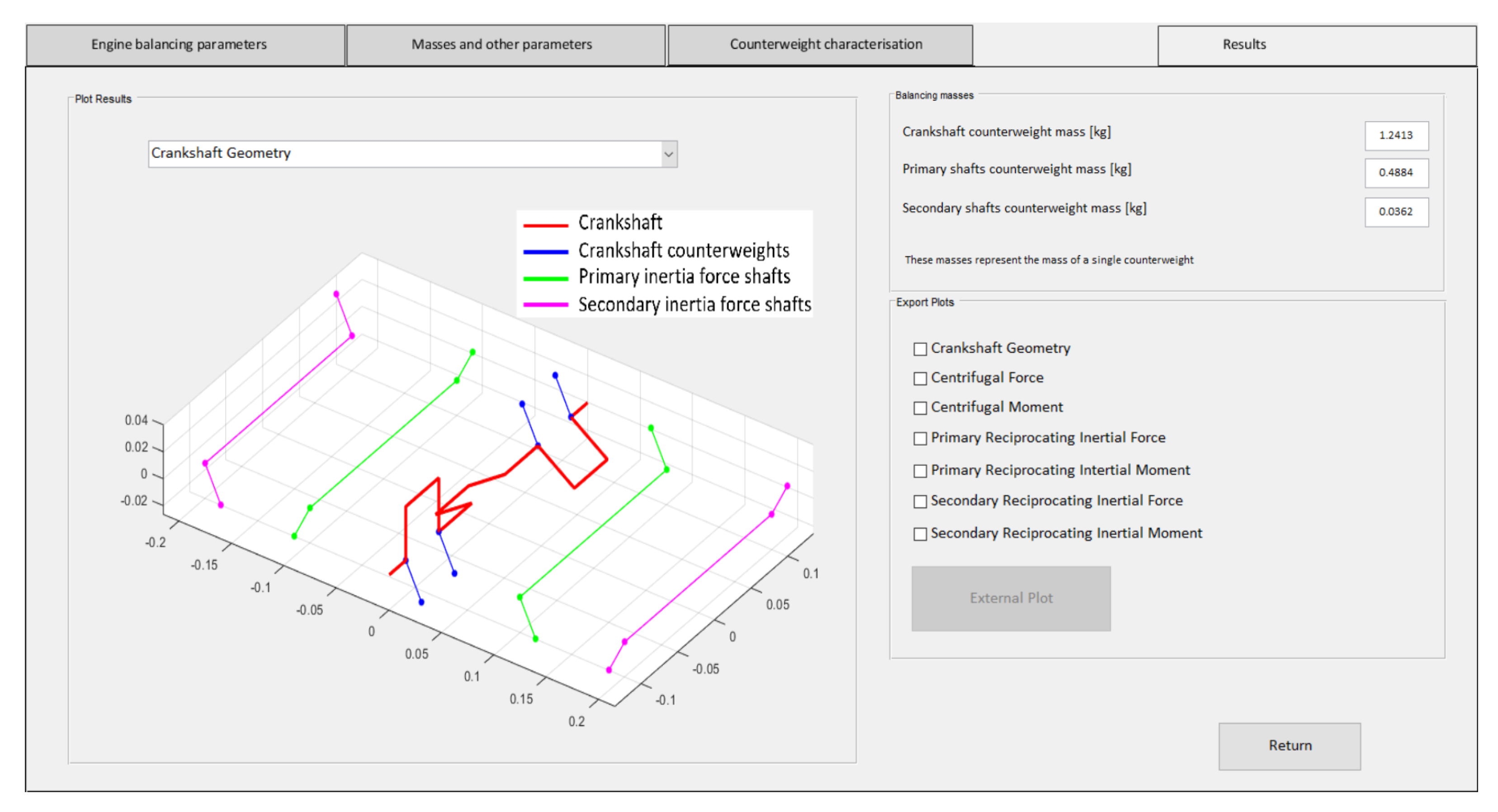
The results computed by the main code are grouped in the fourth tab of the interface, named “Results”. As shown in Figure 9, three panels are included: the first one, called “Plot results”, allows one to visualise the plots for the crankshaft geometry and the resultants for all the forces and moments relative to the balancing process. Such plots enable the user to quickly check the correctness of the process and how the elements are positioned relative to each other. The second panel reports the masses for each balancing counterweight. Finally, the last panel allows for the export of the plots previously presented as separate MATLAB figures. When the results have been checked, the “Return” button allows one to immediately return to the first tab, so that the user can perform again the balancing computations with new inputs.

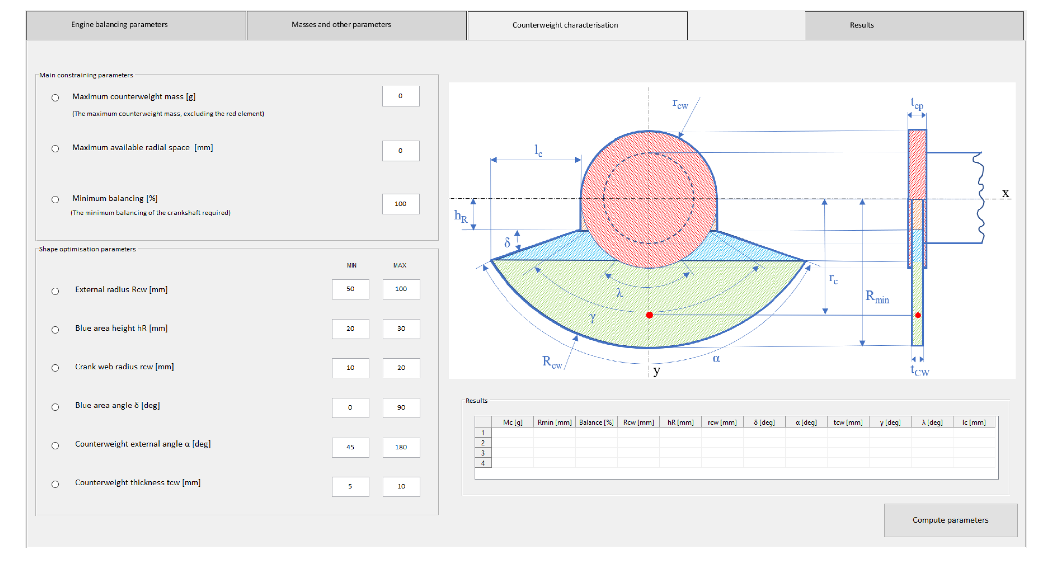
The last tab included in the interface is relative to the characterisation of the counterweights of the crankshaft, which can be used if a more detailed design of the counterweights is desired. This tab, which is reported in Figure 10, uses parts of the main code that is used by the other tabs, with the addition of a specific section, which implements the equations described in Section 4.

It can be noticed that the tab is divided into three panels: two dedicated to the inputs and one to the results. The first one, called “Main constraining parameters”, allows the user to specify the main requirements for the design of the counterweights. These parameters are the most concerning from the design point of view, since they influence the overall performance of the engine:

• The maximum mass of the component;
• The maximum available space for the path of the counterweight permitted by all the other components of the engine;
• The minimum balance requested by the engine.

The second panel groups a set of inputs related to the fine-tuning of the geometry of the counterweight. It is possible to specify a range of limiting values for each parameter which defines the shape of the counterweight. It can be noticed that on the left of each input a selector button has been included: it is used to select which are the parameters that the user wants to modify while the code will have total freedom in what values the others can have. In fact, the code, through the equations defined earlier, will compute all the parameters that characterise the counterweight based on the limiting factors defined by the user. However, it is possible to find multiple solutions (defined as multiple combinations of parameters) for a set of inputs. Therefore, the third panel, called “Results”, will group all the solutions found by the code which respect the constraints imposed. Of course, the more restrictive the inputs, the lower the number of possible solutions and vice versa.

6. Practical Examples

In order to demonstrate the balancing process of the tool, a 3 cylinders in-line and a 4 cylinders V90° engine will be shown.

6.1. 3 Cylinder in-Line Engine

Regarding the preliminary balancing, once the inputs for the configuration, which can be seen in

Table 1. Input data for the optimisation of a 3 cylinder in-line engine.

Engine Type	${\mathit{N}}_{\mathit{cyl}}$	Firing Order	$\mathit{\varphi }$[deg]	a [mm]	${\mathit{N}}_{\mathit{cw}}$	${\mathit{N}}_{\mathit{cw},1}$	${\mathit{N}}_{\mathit{cw},2}$	${\mathit{N}}_{\mathit{sh},1}$	${\mathit{N}}_{\mathit{sh},2}$	${\mathit{r}}_{\mathit{c}}$[mm]	${\mathit{r}}_{\mathit{c},1}$[mm]
In-line	3	1,3,2	120	90	4	2	2	2	2	30	30
${\mathit{L}}_{\mathit{sh},\mathbf{1},\mathit{r}}$  [mm]	${\mathit{L}}_{\mathit{sh},\mathbf{2},\mathit{r}}$  [mm]	${\mathit{L}}_{\mathit{sh},\mathbf{1},\mathit{cr}}$	${\mathit{L}}_{\mathit{sh},\mathbf{2},\mathit{cr}}$	$\mathit{\omega }$  [rpm]	$\mathit{D}$  [mm]	$\mathit{r}$  [mm]	${\mathit{l}}_{\mathit{cr}}$  [mm]	${\mathit{z}}_{\mathit{oc}}$  [mm]	${\mathit{z}}_{\mathit{owp}}$  [mm]	${\mathit{m}}_{\mathit{p}}$  [g]	${\mathit{m}}_{\mathit{wp}}$  [g]
100	200	−100	−200	2000	80	40	135	0	500	240
${\mathit{m}}_{\mathit{cr}}$  [g]	${\mathit{r}}_{\mathit{c},\mathbf{2}}$  [mm]	${\mathit{l}}_{\mathit{sh},\mathbf{1}}$	${\mathit{l}}_{\mathit{sh},\mathbf{2}}$	${\mathit{m}}_{\mathit{cp}}$  [g]	${\mathit{m}}_{\mathit{cw}}$  [g]	${\mathit{r}}_{\mathit{cw}}$   [mm]
600	30	200	200	400	1800	15

, are inserted in the relative tabs (1 and 2), the computation can be started. The numerical results, i.e., the counterweights mass, are reported in

Table 2. Balancing masses for a 3 cylinder in-line engine.

${\mathit{m}}_{\mathit{c}}$ [kg]	${\mathit{m}}_{\mathit{c},1}$ [kg]	${\mathit{m}}_{\mathit{c},2}$ [kg]
1.2413	0.4884	0.0362

.

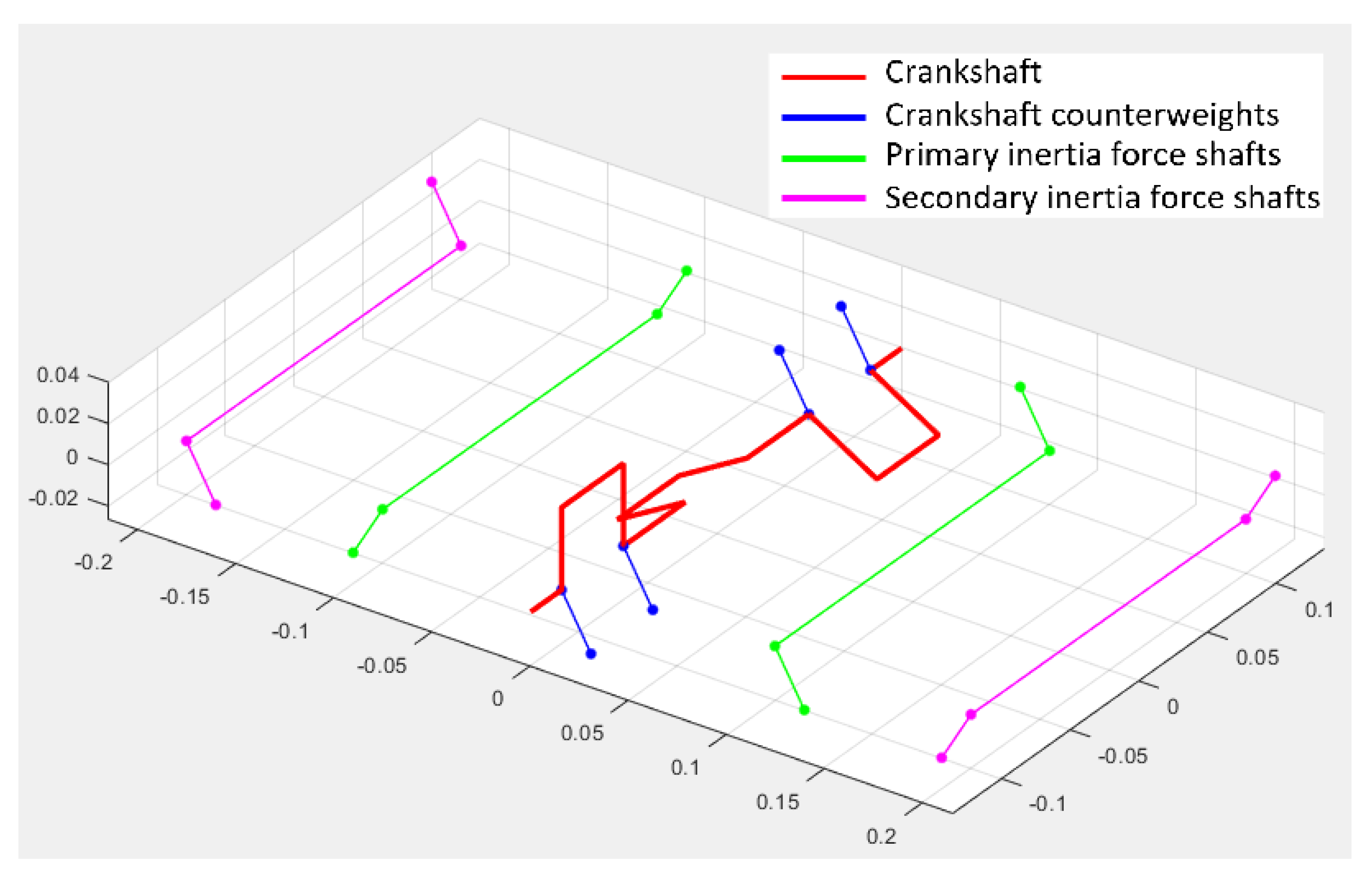
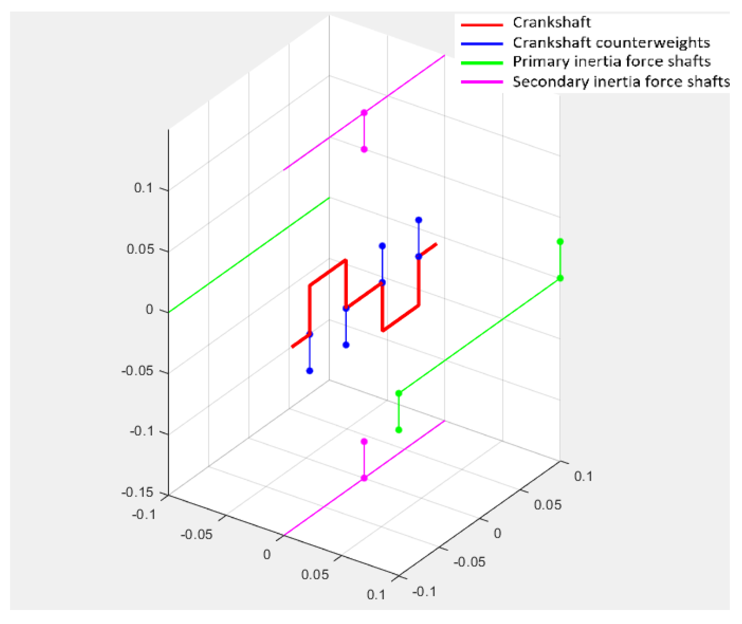
The highest value obtained is the one relative to the crankshaft counterweights: this fact is expected, since, looking at the input data, the rotating masses are larger than the reciprocating ones. Moreover, the mass for the secondary reciprocating forces is quite a small value relative to the others. Therefore, avoiding the secondary balancing shafts may be an option, which would reduce the overall complexity of the engine. The geometry of the defined configuration is shown in Figure 11.

The geometry corresponds to the most used configuration of a 3 cylinder engine. It is also noticeable that the crankshaft counterweights are not symmetrical to their relative crank. It should be noted that, by convention, the geometry is shown with the first crank exhibiting a crank angle equal to zero ($\theta =0$).

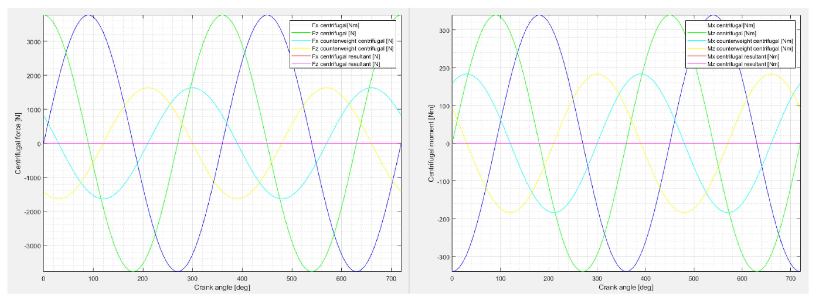
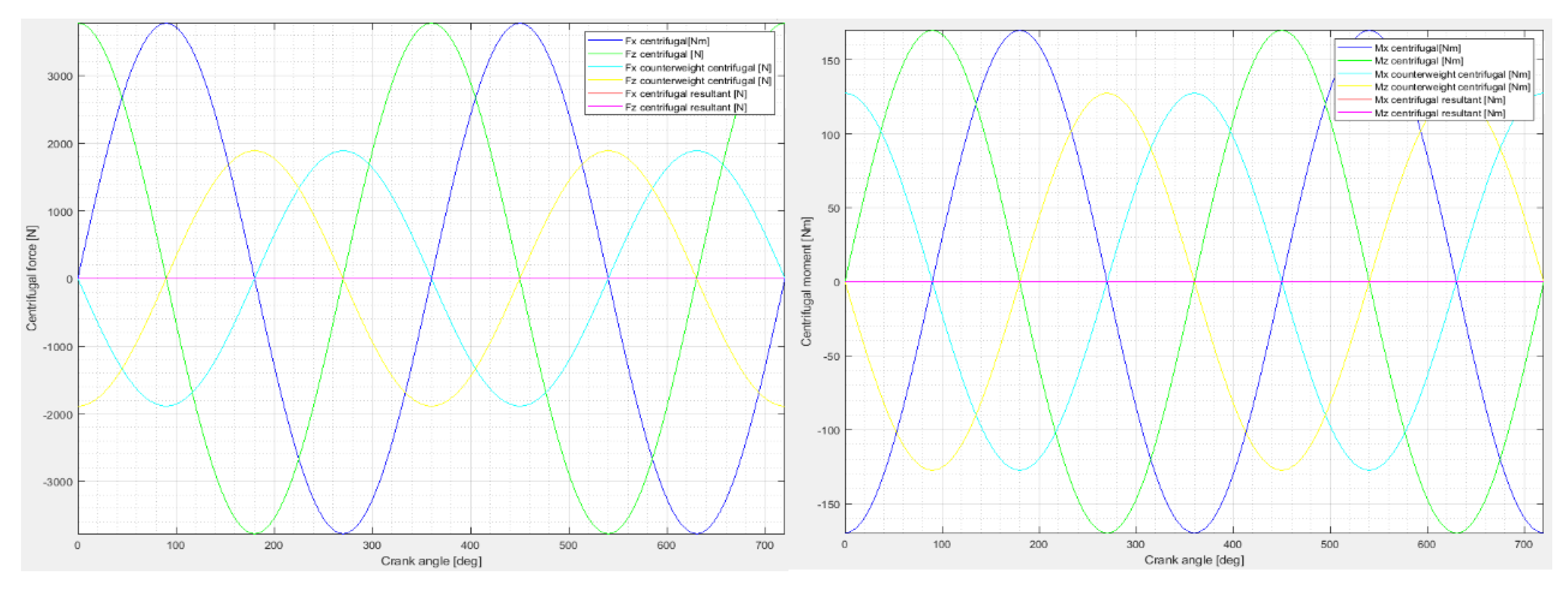
The plots for the equilibrium of the centrifugal forces and moments, with their x and z components, are reported in Figure 12.

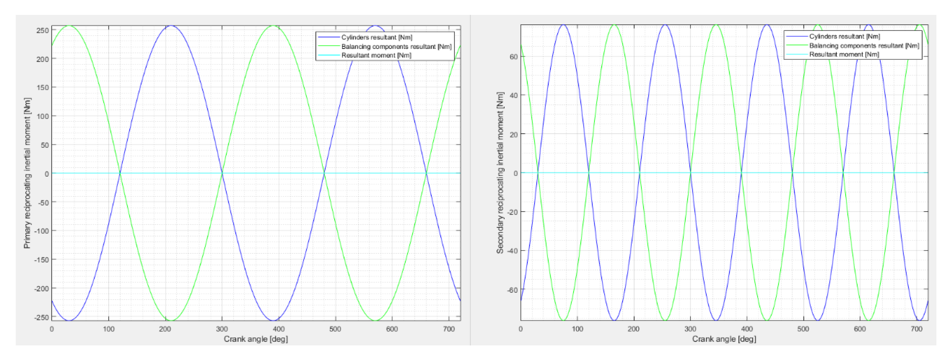
It is possible to see that the application of the counterweights allows one to cancel the resultants and, therefore, to balance the crankshaft. A similar argument can be made for the reciprocating moments, both primary and secondary. Their plots are shown in Figure 13.

It is noticeable that the curves in each plot are symmetrical around the x-axis, allowing for the cancellation of the resultants. This phenomenon can be further confirmed by the geometry plot: in fact, all the balancing shafts have an opposite counterweights configuration, which allows one to counter the moments.

Finally, an optimisation, through an evolutionary algorithm, of the counterweights to be added on the crankshaft, in order to balance it centrifugally, can be performed through the third tab, presented in Section 5. The input values used are those reported in Figure 10, while the results obtained are shown in

Table 3. Results for two optimisations of the counterweights.

Optimisation	CW Mass [g]	${\mathit{R}}_{\mathit{min}}$ [mm]	Balance [%]	${\mathit{R}}_{\mathit{cw}}$ [mm]	${\mathit{h}}_{\mathit{R}}$ [mm]	${\mathit{r}}_{\mathit{cw}}$ [mm]	$\mathit{\delta }$ [rad]	$\mathit{\alpha }$ [rad]	${\mathit{t}}_{\mathit{cw}}$ [mm]	$\mathit{\gamma }$ [rad]	$\mathit{\delta }$ [rad]	${\mathit{l}}_{\mathit{c}}$ [mm]
$M_c$ Minimisation	117.46	161.67	99.90	50.04	29.97	10.01	1.46	0.79	5.00	0.00	0.00	9.28
$R_{min}$ Minimisation	196.80	70.00	99.99	50.00	20.00	20.00	0.00	3.13	6.05	0.00	0.00	30.00

. For what concerns the input data relative to the crankshaft, the set shown in Figure 8 is used.

The optimisation reported is obtained by imposing a perfect balance of the crankshaft (100% Balance), so that the code will find all the solutions abiding by this constraint. From these solutions, the most relevant ones are highlighted: the one with the minimum mass (CW mass) and the one with the maximum possible radial size ($R_{min}$), reported in Table 1 as “MIN Mass” and “MIN Clearance”, respectively. Alongside these two parameters, it is possible to see all the other geometrical dimensions, computed by the code, which define the geometry of the counterweight, and, therefore, complete its characterisation.

6.2. 4 Cylinder V-Engine

The second example presented will be a 4 cylinder V-engine with a 90° bank angle. The setup procedure is the same as the 3 cylinder case; however, for sake of brevity, the counterweight characterisation is not performed for this configuration. In

Table 4. Input data for the optimisation of a 4 cylinder V-engine.

Engine Type	${\mathit{N}}_{\mathit{cyl}}$	Firing Order	$\mathit{\varphi }$[deg]	a [mm]	${\mathit{N}}_{\mathit{cw}}$	${\mathit{N}}_{\mathit{cw},1}$	${\mathit{N}}_{\mathit{cw},2}$	${\mathit{N}}_{\mathit{sh},1}$	${\mathit{N}}_{\mathit{sh},2}$	${\mathit{r}}_{\mathit{c}}$[mm]	${\mathit{r}}_{\mathit{c},1}$[mm]
V	4	1,4,3,2	180	90	4	2	1	2	2	30	30
${\mathit{L}}_{\mathit{sh},\mathbf{1},\mathit{r}}$  [mm]	${\mathit{L}}_{\mathit{sh},\mathbf{2},\mathit{r}}$  [mm]	${\mathit{L}}_{\mathit{sh},\mathbf{1},\mathit{cr}}$	${\mathit{L}}_{\mathit{sh},\mathbf{2},\mathit{cr}}$	$\mathit{\omega }$  [rpm]	$\mathit{D}$  [mm]	$\mathit{r}$  [mm]	${\mathit{l}}_{\mathit{cr}}$  [mm]	${\mathit{z}}_{\mathit{oc}}$  [mm]	${\mathit{z}}_{\mathit{owp}}$  [mm]	${\mathit{m}}_{\mathit{p}}$  [g]	${\mathit{m}}_{\mathit{wp}}$  [g]
100	200	−100	−200	2000	80	40	135	0	500	240
${\mathit{m}}_{\mathit{cr}}$  [g]	${\mathit{r}}_{\mathit{c},\mathbf{2}}$  [mm]	${\mathit{l}}_{\mathit{sh},\mathit{1}}$	${\mathit{l}}_{\mathit{sh},\mathbf{2}}$	${\mathit{m}}_{\mathit{cp}}$  [g]	${\mathit{m}}_{\mathit{c}\mathit{w}}$ [g]	${\mathit{r}}_{\mathit{cw}}$  [mm]	$\mathbf{\alpha }$  [deg]
600	30	200	200	400	1800	15	90

the input data used can be visualised, while in

Table 5. Balancing masses for a 4 cylinder V-engine.

${\mathit{m}}_{\mathit{c}}$ [kg]	${\mathit{m}}_{\mathit{c},1}$ [kg]	${\mathit{m}}_{\mathit{c},2}$ [kg]
1.700	0.3948	0.1299

the corresponding output data is inserted. Since the inputs used are very similar to the 3 cyilinder engine ones, a comparison can be done: it is noticeable that the crankshaft counterweights, in charge of balancing the centrifugal components, have higher mass due to the higher rotational mass derived from the additional cylinder. Instead, the counterweights mass for the primary reciprocating moment is smaller, even though the number of cylinders is higher, due to the lower distance of each crank mid-point from the mid-plane of the crankshaft.

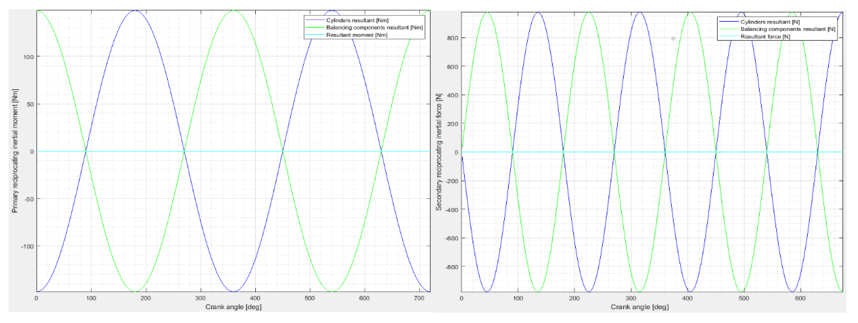
In Figure 14 the geometry plot can be visualised. It is noticeable that the configuration is very similar to a 2 cylinder in-line engine, but the code correctly accounts for the presence of 2 conrod and pistons for each crank. From Figure 15, the balancing of the centrifugal forces and moments can be seen, and, similarly, to the 3 cylinder example, the resultant curves (in magenta) are completely flat. The same discussion can be made for the other characteristics that need balancing, in particular the primary reciprocating moment and the secondary reciprocating force, which are reported in Figure 16.

7. Conclusions

The proposed design tool is successful in identifying the masses and the configuration of the counterweights necessary for the dynamic balance of the crankshaft of an internal combustion engine. Unlike existing codes, which typically specialise on a given engine configuration, the proposed matrix formulation is fit to address the majority of engine configurations. The rationalisation and unification of the framework used to describe the different engine configurations not only makes the tool very flexible but also ensures meaningful results in a very short time. Such results can be easily double-checked by the user, both from a geometry standpoint and in quantitative balance terms. Moreover, the implementation of the counterweight characterisation allows the complete definition of the counterweight shape according to the most significant optimisation criteria, e.g., minimum weight and minimum clearance. Finally, the creation of a user-interface for the code enhances the usability of the tool, simplifying the input insertion process.

References

- Kirwan, J.E.; Shost, M.; Roth, G.; Zizelman, J. 3-Cylinder Turbocharged Gasoline Direct Injection: A High Value Solution for Low CO2 and NOx Emissions. SAE Int. J. Engines 2010, 3, 355–371. [Google Scholar] [CrossRef]
- Delprete, C.; Razavykia, A. Piston ring–liner lubrication and tribological performance evaluation: A review. Proc. Inst. Mech. Eng. Part J J. Eng. Tribol. 2017, 232, 193–209. [Google Scholar] [CrossRef]
- Manzie, C. Relative Fuel Economy Potential of Intelligent, Hybrid and Intelligent–Hybrid Passenger Vehicles. In Electric and Hybrid Vehicles; Elsevier: Hoboken, NJ, USA, 2010; pp. 61–90. [Google Scholar] [CrossRef]
- Ecker, H.J.; Schwaderlapp, M.; Gill, D.K. Downsizing of Diesel Engines: 3-Cylinder/4-Cylinder. In SAE Technical Paper Series; SAE International: Warrendale, PA, USA, 2000. [Google Scholar] [CrossRef]
- Victor, W. Machinery Vibration: Balancing; McGraw-Hill Professional: New York, NY, USA, 1998. [Google Scholar]
- Albers, A.; Leon-Rovira, N.; Aguayo, H.; Maier, T. Development of an engine crankshaft in a framework of computer-aided innovation. Comput. Ind. 2009, 60, 604–612. [Google Scholar] [CrossRef]
- Quinsat, Y.; Lartigue, C. Filling holes in digitized point cloud using a morphing-based approach to preserve volume characteristics. Int. J. Adv. Manuf. Technol. 2015, 81, 411–421. [Google Scholar] [CrossRef]
- Guarato, A.Z.; Quinsat, Y.; Mehdi-Souzani, C.; Lartigue, C.; Sura, E. Conversion of 3D scanned point cloud into a voxel-based representation for crankshaft mass balancing. Int. J. Adv. Manuf. Technol. 2017, 95, 1315–1324. [Google Scholar] [CrossRef] [Green Version]
- Kang, Y.; Tseng, M.H.; Wang, S.M.; Chiang, C.P.; Wang, C.C. An accuracy improvement for balancing crankshafts. Mech. Mach. Theory 2003, 38, 1449–1467. [Google Scholar] [CrossRef]
- Schnurbein, E.V. A New Method of Calculating Plain Bearings of Statically Indeterminate Crankshafts. In SAE Technical Paper Series; SAE International: Warrendale, PA, USA, 1970. [Google Scholar] [CrossRef]
- Razavykia, A.; Delprete, C.; Baldissera, P. Numerical Study of Power Loss and Lubrication of Connecting Rod Big-End. Lubricants 2019, 7, 47. [Google Scholar] [CrossRef] [Green Version]
- Parikyan, T.; Resch, T. Statically Indeterminate Main Bearing Load Calculation in Frequency Domain for Usage in Early Concept Phase. In ASME 2012 Internal Combustion Engine Division Fall Technical Conference; American Society of Mechanical Engineers: New York, NY, USA, 2012. [Google Scholar] [CrossRef]
- Stanley, R.; Taraza, D. A Characteristic Parameter to Estimate the Optimum Counterweight Mass of a 4-Cylinder In-Line Engine. In SAE Technical Paper Series; SAE International: Warrendale, PA, USA, 2002. [Google Scholar] [CrossRef]
- Rosso, C.; Delprete, C.; Bonisoli, E.; Tornincasa, S. Integrated CAD/CAE Functional Design for Engine Components and Assembly. In SAE Technical Paper Series; SAE International: Warrendale, PA, USA, 2011. [Google Scholar] [CrossRef]
- Albers, A.; Leon, N.; Aguayo, H.; Maier, T. Comparison of Strategies for the Optimization/Innovation of Crankshaft Balance. In IFIP The International Federation for Information Processing; Springer: New York, NY, USA, 2007; pp. 201–210. [Google Scholar] [CrossRef] [Green Version]
Figure 1.
Model of the crankshaft for a 3 cylinder in-line engine, with the relative polar plot on the right.
Figure 2.
Isometry and relative polar plot of the crankshaft for a 3 cylinder in-line engine, including the centrifugal forces equilibrium.
Figure 3.
Polar plot and relative isometry of the crankshaft for a 2 cylinder in-line engine with a 180° angle between cranks, including the primary reciprocating forces equilibrium and the additional primary balancing shafts.
Figure 4.
Polar plot and relative isometry of the crankshaft for a 2 cylinder in-line engine with a 180° angle between cranks, including the secondary reciprocating forces equilibrium and the additional secondary balancing shafts.
Figure 5.
Model and quotas of the crankshaft counterweight.
Figure 6.
Examples of characterisation of a crankshaft counterweight.
Figure 7.
Tab of the user-interface dedicated to the insertion of the general and balancing input data.
Figure 8.
Tab of the user-interface devoted to the definition of the geometrical parameters and the masses of the crank mechanism.
Figure 9.
Tab of the user-interface dedicated to the preliminary balancing results.
Figure 10.
Tab of the user-interface dedicated to the design and optimisation of the counterweights.
Figure 11.
Geometry of crankshaft and balancing shafts for a 3 cylinder in-line engine.
Figure 12.
Centrifugal forces (left) and moments (right) for a 3 cylinder in-line engine.
Figure 13.
Primary (left) and secondary (right) reciprocating moments for a 3 cylinder in-line engine.
Figure 14.
Geometry of crankshaft and balancing shafts for a 4 cylinder V-engine.
Figure 15.
Centrifugal forces (left) and moments (right) for a 4 cylinder V-engine.
Figure 16.
Primary reciprocating moment (left) and secondary reciprocating force (right) balancing curves for a 4 cylinder V-engine.