Article

Power Quality Analysis of the Output Voltage of AC Voltage and Frequency Controllers Realized with Various Voltage Control Techniques

1
Department of Electrical Engineering, The University of Lahore, Lahore 54000, Pakistan
2
Department of Electrical Engineering, College of Engineering, University of Ha’il, Hail 1234, Saudi Arabia
3
Department of Industrial Engineering, College of Engineering, University of Ha’il, Hail 1234, Saudi Arabia
*
Author to whom correspondence should be addressed.
Submission received: 27 November 2020 / Revised: 2 January 2021 / Accepted: 5 January 2021 / Published: 7 January 2021

Abstract

:
Single-phase and three-phase AC-AC converters are employed in variable speed drive, induction heating systems, and grid voltage compensation. They are direct frequency and voltage controllers having no intermediate power conversion stage. The frequency controllers govern the output frequency (low or high) in discrete steps as per the requirements. The voltage controllers only regulate the RMS value of the output voltage. The output voltage regulation is achieved on the basis of the various voltage control techniques such as phase-angle, on-off cycle, and pulse-width modulation (PWM) control. The power quality of the output voltage is directly linked with its control techniques. Voltage controllers implemented with a simple control technique have large harmonics in their output voltage. Different control techniques have various harmonics profiles in the spectrum of the output voltage. Traditionally, the evaluation of power quality concerns is based on the simulation platform. The validity of the simulated values depends on the selection of the period of a waveform. Any deficiency in the selection of the period leads to incorrect results. A mathematical analytical approach can tackle this issue. This becomes important to analytically analyze the harmonious contents generated by various switching control algorithms for the output voltage so that these results can be successfully used for power quality analysis and filtering of harmonics components through various harmonics suppression techniques. Therefore, this research is focused on the analytical computation of the harmonics coefficients in the output voltage realized through the various voltage and frequency control techniques. The mathematically computed results are validated with the simulation and experimental results.

1. Introduction

1.1. Problem Statement

Power quality is one of the major concerns in today’s modern power system. In traditional generation and distribution systems, the issue of low power quality is meaningless as the connected load is linear such as incandescent lamps and heating load. The speed of the rotating loads is governed via their voltage control that is achieved through conventional approaches. That includes the use of auto-transformers, transformer tap-changing mechanisms, and variable resistance. These power control mechanisms are inefficient and are replaced with switching converters nowadays. The power electronic converters are plying a vital role in the development of modern-day life by converting one form of electric power into another form. The converted output in the power conversion process is not always in the pure form and includes unwanted components called harmonics. The nature of unwanted harmonics deteriorating the power quality should be known before employing different harmonics mitigation and compensation methods. This research focuses on the mathematical computation of the harmonic components analytically and then the validation of mathematically computed results through simulation and experimental results.

1.2. Literature Review

Reference [1] pin-points that the source of the harmonics in the power system is owing to the use of non-linear loads that include battery charging system, smart refrigerating and air-conditioning systems, computers, electric furnaces, and fluorescent or LED lighting systems. The current drawn by the non-linear loads or devices is non-linear which leads to poor power quality issues. This non-linear current to be supplied by the input source flows through the entire power system. This may interact with the capacitance and inductance of the system. Therefore, the generated harmonics is one of the major concerns and challenging issues that leads the male functioning of the connected and protection systems, and reliability concerns of devices and components in the power system [2]. They also increase the neutral current in a three-phase power system [3]. They become more serious once they interact with the grid or system’s inductance. Therefore, this problem is a major resonance source for poor power quality and instability concerns in the power system. All industrial consumers are forced to improve their produced negative footprint through power compensating topologies. Therefore, the harmonic analysis becomes one of the main concerns for performance evaluation of the power converting systems.
The profile of the generated harmonics in the power conversion process is directly linked with the type and switching algorithm of the power processing units. The power quality of the grid or load voltage may be improved through the harmonic elimination techniques. The generated harmonics may be tackled at the unit level or system level [4,5]. Normally, passive [6,7] and active filters [8,9,10,11] are employed to suppress them. The selection of cutoff frequency or bandwidth depends on the frequency of the dominant harmonics. The harmonics elimination through passive filter approaches is normally employed in low power to medium power applications as they are simple and reliable. Here, the basic key is to divert the unwanted components or block them through a high impedance. These techniques may include series, parallel or hybrid filters. In parallel filter techniques, the propagation of generated harmonics is blocked to move towards the source by establishing a low impedance path across the load. In series compensating techniques, harmonics are blocked due to the high impedance of series compensators. The harmonics suppression through traditional DC link capacitors is bulky and unreliable and therefore, this approach is not cost-effective. These issues are tackled in the slim type DC link capacitors as reported in [12]. Here, the magnitude of the harmonics is only evaluated without considering their phase. Their harmonics suppression characteristics at the system level are not improved as they may be achieved with traditional power converting topologies realized with DC or AC filters (choke). The power converting topologies realized with slim type DC link capacitors have improved harmonics suppression capabilities once they are connected in parallel with other power converters. In the AC to DC conversion process, the higher pulse rectifier’s topologies may also be employed but their use is restricted to some applications due to their complex circuit arrangement [13,14,15,16]. The mathematical computation of output voltage and input current harmonics of a six-pulse rectifier is reported in [17] but they are not practically validated. The harmonic profile of various outputs of power converting systems is practically evaluated in [1,18].
The variation in the magnitude and phases of harmonics is observed due to the use of a DC-link capacitor or DC and AC chokes [19,20]. It is investigated in [21] that the phase angles of the three-phase and single-phase for the fifth harmonic are equal and opposite at the unit level. But there may be some variation in their phase once the number of power converting systems is connected to the same coupling point. The harmonics suppression through the paralleling of power converters requires a large number of power converters. This approach cannot be employed in the case where a converter is feeding power to an individual load.
The direct AC-AC converters are more attractive over the sizeable indirect AC-AC converters (AC-DC-AC converters) as their operation is accomplished through single-stage power conversion. They are the more viable choice in most applications, such as motor speed drive, grid voltage compensation [22,23,24], and induction heating systems [25,26]. Thyristor-based AC voltage controllers are used at the domestic level for speed regulation of the fans. They are also employed in some industrial drives. These topologies are simple to implement but they have certain serious drawbacks. The RMS values of the output voltage are controlled via the control of the firing delay. They have a problem of low order harmonics as the switching frequency is equal to the input source. That increases the total harmonic distortion (THD) and reduces the power factor (PF). On-off cycle control is another approach to control the output RMS voltage with the load having a high time constant. For example, heavy industrial load having a high mechanical time constant, or heating load having a high thermal time constant. This voltage control topology is also realized with thyristor-based converters. Here the switching of a thyristor is accomplished at zero crossings of the input voltage. The amplitude of the fundamental component and generated harmonics depends upon the number of on and off cycles. The generated harmonics also exist at low frequencies that cannot be easily suppressed. The generated harmonics are shifted at higher frequencies in the power converter implemented with the pulse-width modulation (PWM) approach by increasing the switching frequencies of operating devices [27]. The high-frequency harmonics can be easily eliminated by employing a low pass filter. The output voltage regulation is governed through the duty cycle control of the PWM signals. The AC voltage controller operated with bipolar voltage gain may regulate the output frequencies in discrete steps. This is accomplished by operating the converters in non-inverting and inverting modes according to the output frequency requirements [25,26].
The output voltage and frequency control are realized through various switching schemes and converting topologies. Each switching scheme or power converting topology has a distinctive harmonic profile. Conventionally, the harmonic analysis based on FFT is employed in [28,29,30,31] for harmonic analysis but it has the problem of aliasing and spectrum leakage as it is based on sampling frequency and window. The selection of the period of the wave is also a critical issue and it leads to incorrect results. The double Fourier series is employed in the Jacobi matrix [32] but its spectrum analysis is inaccurate as only two frequencies from the input, output, and sampling are considered. This problem is tackled in the triple Fourier series as in [33] but this approach is not mature due to some deficiencies. These approaches are employed in indirect AC-AC converters and cannot be employed in direct AC-AC converters due to complex mathematics. The harmonics of an uncontrolled three-phase rectifier are computed through sample delta and state-space approach in [34,35] but these approaches are complex to apply in other power converting topologies. A novel approach for harmonic analysis is reported in [36] for a rectifier circuit realized through a multi-pulse approach. Here the three input phase currents are converted in the form of a stepped wave by employing the paralleling of four converters. The harmonics contents of each converter are suppressed through their elimination topologies. The harmonics contents of AC-AC converters are usually addressed in Simulink’s dependent environment.

1.3. Research Contribution

Existing mathematical tools that are employed to explore the power quality concerns of the inverters (DC-AC converters) become complicated if they are used in power quality concerns of direct AC-AC converters. An accurate analytical and simple approach that we call pulse selective approach (PSA) as reported in [17,26] is employed to compute the harmonic contents for AC-DC converters and direct frequency changers but they are not yet practically validated. In this approach, a waveform that apparently seems to be non-sinusoidal is decomposed to its parents’ sinusoidal components during some selected periods of time. The power quality concerns of each sinusoidal wave in the selected period are evaluated; then their results are merged to have the harmonic contents of that entire waveform. According to the authors’ best knowledge, this approach is not employed for power quality evaluation in the direct single-phase and three-phase AC voltage controllers. Therefore, in this research article, the harmonics contents of the output voltage for various AC voltage control schemes are analytically computed. The computed harmonics contents are validated through practical and simulation results. The MATLAB/Simulink based environment is employed to simulate the harmonics contents for direct AC-AC converters by carefully selecting the period as an inaccurate selection of the period of a waveform leads to inaccurate results. In a nutshell, the contribution of this research article is the successful application of the proposed (analytical) pulse selective approach to AC-AC voltage converters for computing harmonic contents and then the validation of mathematically computed results through simulation and experimental results.

1.4. Paper Organization

The arrangement of this research article includes the description of the pulse selective approach (PSA) in Section 2, followed by the harmonics coefficients computation in Section 3, Section 4 and Section 5. Section 6 validates the computed values with the results obtained through simulation and practical values. The conclusion is explored in Section 7.

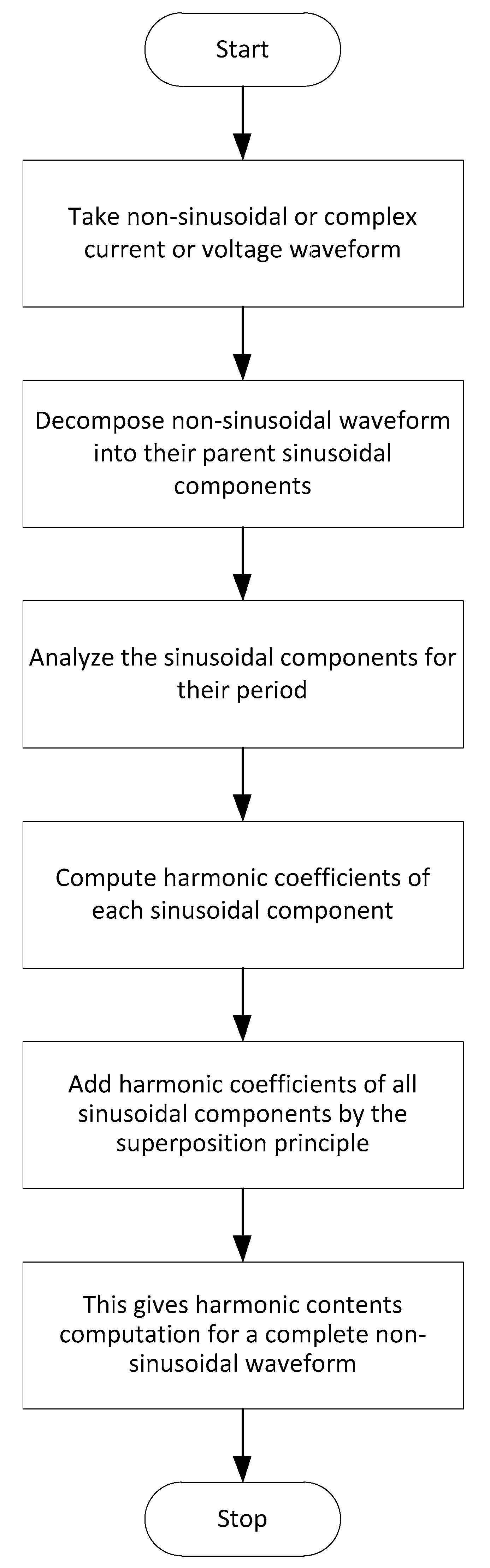
2. Pulse Selective Approach

This analytical approach is one of the simplest methods to evaluate the power quality concerns of current or voltage waveforms that apparently seem to be non-sinusoidal or complex. The non-sinusoidal nature of waveforms is due to the switching mechanism involved in the switching converters. That may invert, non-invert, or chop the input voltage waveform at the output in a single-phase supply system. This may also be due to the summation or subtraction of the input voltage sources at the output in a three-phase supply system. Thus, it results in harmonic contents. So, a resultant non-sinusoidal voltage or current waveform is a series of various harmonic frequencies.
In the pulse selective approach (PSA), such non-sinusoidal current or voltage waveforms are decomposed into their parent sinusoidal components. Then each component is analyzed for its period that is required to compute its harmonic coefficients. The harmonic coefficients of each sinusoidal component present in the considered (current or voltage) waveform are computed. The harmonic coefficients of all sinusoidal components are added by the superposition principle to have the harmonic coefficients of a complete waveform. This way, well-distinct numerical expressions of non-sinusoidal currents and voltages are obtained to compute the harmonics. The steps involved in the PSA are presented in the form of a flow chart shown in Figure 1.
It should be remembered that the selection of a period is quite crucial. For example, in the case of direct AC-AC and AC-DC converters, the period of the input voltage waveform is always ‘2π’, but the periods of the output voltage or current waveforms may or may not be ‘2π’. To add more insight, the outputs of the frequency controllers for double and half frequency become periodic after ‘π’ and ‘4π’ intervals respectively. For these outputs, the period of the required components is equal to the period of the instantaneous waveform but this is not always true. For example, the voltage waveform where the required output frequency is three times the input voltage frequency, the period of the required component (voltage component having frequency three times the input frequency) and instantaneous output voltage waveform is one third and is equal to the period of the input voltage waveform respectively. The periods of these sinusoidal components are chosen by analyzing them for zero average value during selected periods.
As can be seen, the PSA needs not to involve look-up tables, Bessel functions, and numerical techniques for the computation of harmonic magnitude and angle. Realizing this fact, the application of PSA to compute the harmonic contents of non-sinusoidal current and voltage waveforms of AC-AC voltage controllers is presented in the coming sections. The harmonic coefficients for other types of switching converters can also be computed by PSA. Switching mechanism, converter type (single-phase or three-phase), input and output waveform frequencies, and so on result in different current and voltage waveforms.

3. Single-Phase AC Voltage Controllers

They have many control techniques to regulate the RMS value of the output AC voltage. Their detailed and analytical analysis is explored below.

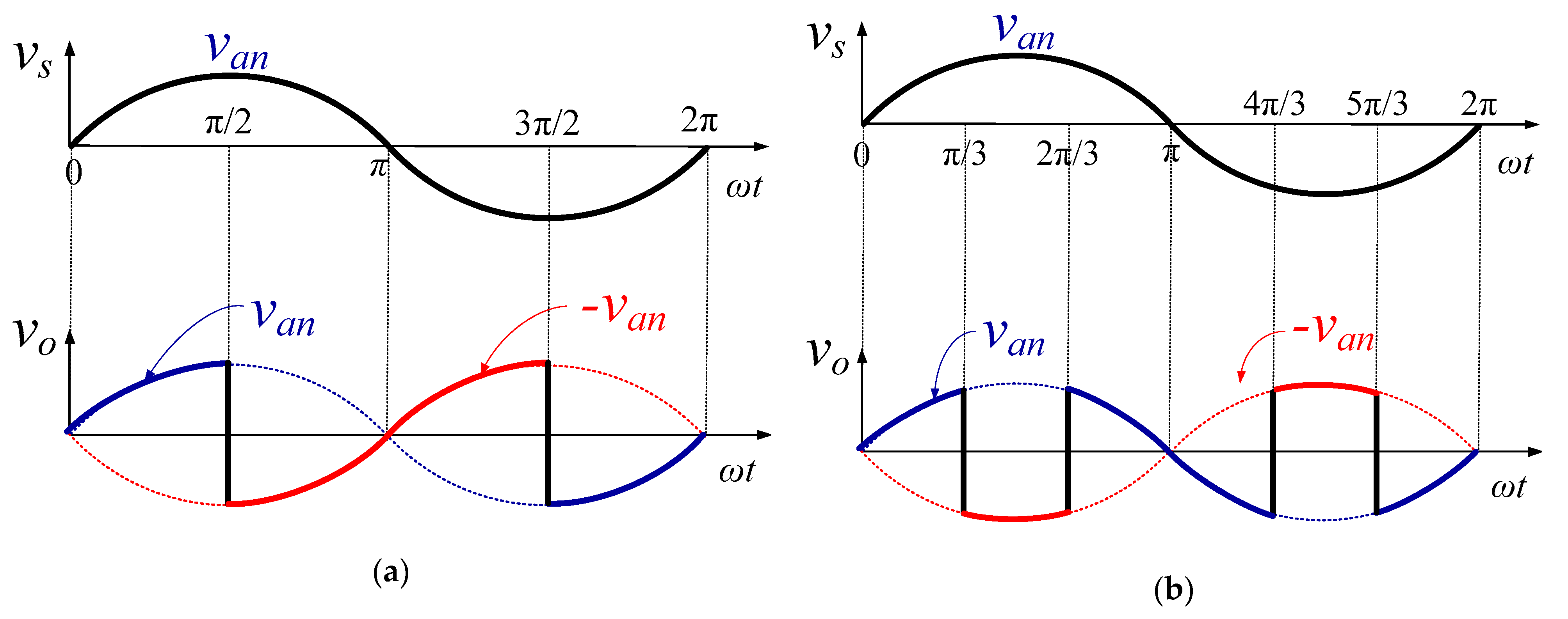
3.1. Phase-Angle Control

This voltage control technique is the simplest to implement, but it contains low-frequency harmonics as the switching frequency is low (equal to the input or output frequency). It has two voltage control schemes depending upon the number of controlled switching devices. The power quality of their output voltage is detailed as.

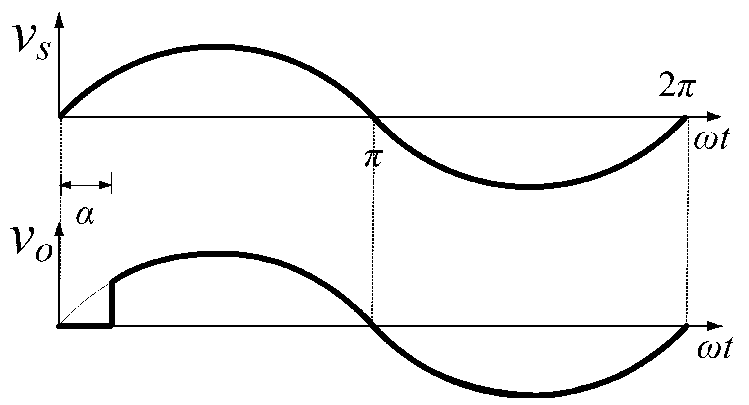
3.1.1. Voltage Regulation with Unipolar Voltage Control Scheme

It is employed in a low power rating load as it contains a DC component. In this output voltage control approach, only one-half cycle of the output voltage is controlled. The other half cycle remains uncontrolled, resulting in the output voltage asymmetric along the vertical (y) axis that causes the generation of the DC component and even harmonics. The output has low-frequency harmonics as the switching devices are operated at low line frequency. Figure 2 depicts the output voltage with respect to the input voltage, where ‘α’ is the firing delay that controls the output voltage only during the positive half cycle of the input voltage. Here ‘vs’ and ‘vo’ are the instantaneous input and output voltage respectively.
With the assumption of sinusoidal input voltage, that is to say
v s = V m sin ( ω t )
As the instantaneous output voltage waveform is asymmetric along the y-axis, the average value of the waveform is non-zero. This average or DC value is computed in the form of harmonic coefficient a0 as
  a 0   = V m 2 π ( 1 cos ( α ) )
This value is varied from ‘0′ to −Vm/π once the firing delay is regulated from ‘0′ to ‘π’. The presence of the asymmetry of the output waveform also results in all even and odd harmonics that can be viewed from the harmonics coefficients an and bn respectively, calculated by
a n [ n 1 ]   =   { V m 2 π ( n 1 ) [ 1 cos ( n α α ) ] V m 2 π ( n + 1 ) [ 1 cos ( n α + α ) ] for   n   =   2 , 3 , 4 , 5 ,
  b n [ n 1 ]   =   { V m 2 π ( n + 1 ) sin ( n α + α ) V m 2 π ( n 1 ) sin ( n α α ) for   n   =   2 , 3 , 4 , 5 ,
These harmonics coefficients are calculated by selecting the period of 2π as the period of the output and input the waves are the same and they are equal to 2π. As the coefficients an and bn become undefined for n = 1, they are separately computed in Equations (5) and (6).
a n [ n = 1 ]   =   V m 4 π [ 1 + cos ( 2 α ) ]
b n [ n = 1 ]   =   V m 2 π [ 2 π α + 1 2 sin ( 2 α ) ]
The closed-form of the instantaneous output voltage in terms of various harmonics contents is realized in Equation (7). This depicts that output has all harmonics as the waveform is asymmetric.
v o ( ω t ) =   V m 2 π [ 1 cos ( α ) ] +   V m 2 π ( 2 π α ) sin ( ω t )   V m 4 π [ cos ( ω t ) cos ( ω t 2 α ) ] + V m 2 π ( n 1 ) [ cos ( n ω t ) cos ( n ω t n α + α ) ]   V m 2 π ( n + 1 ) [ cos ( n ω t ) cos ( n ω t n α α ) ] for   n   =   3 , 5 , 7 ,
The DC (average) component in the output voltage generates a DC component in the input source current that may lead to the core saturation of the transformer connected at the input side. This problem is tackled with a bipolar voltage control scheme.

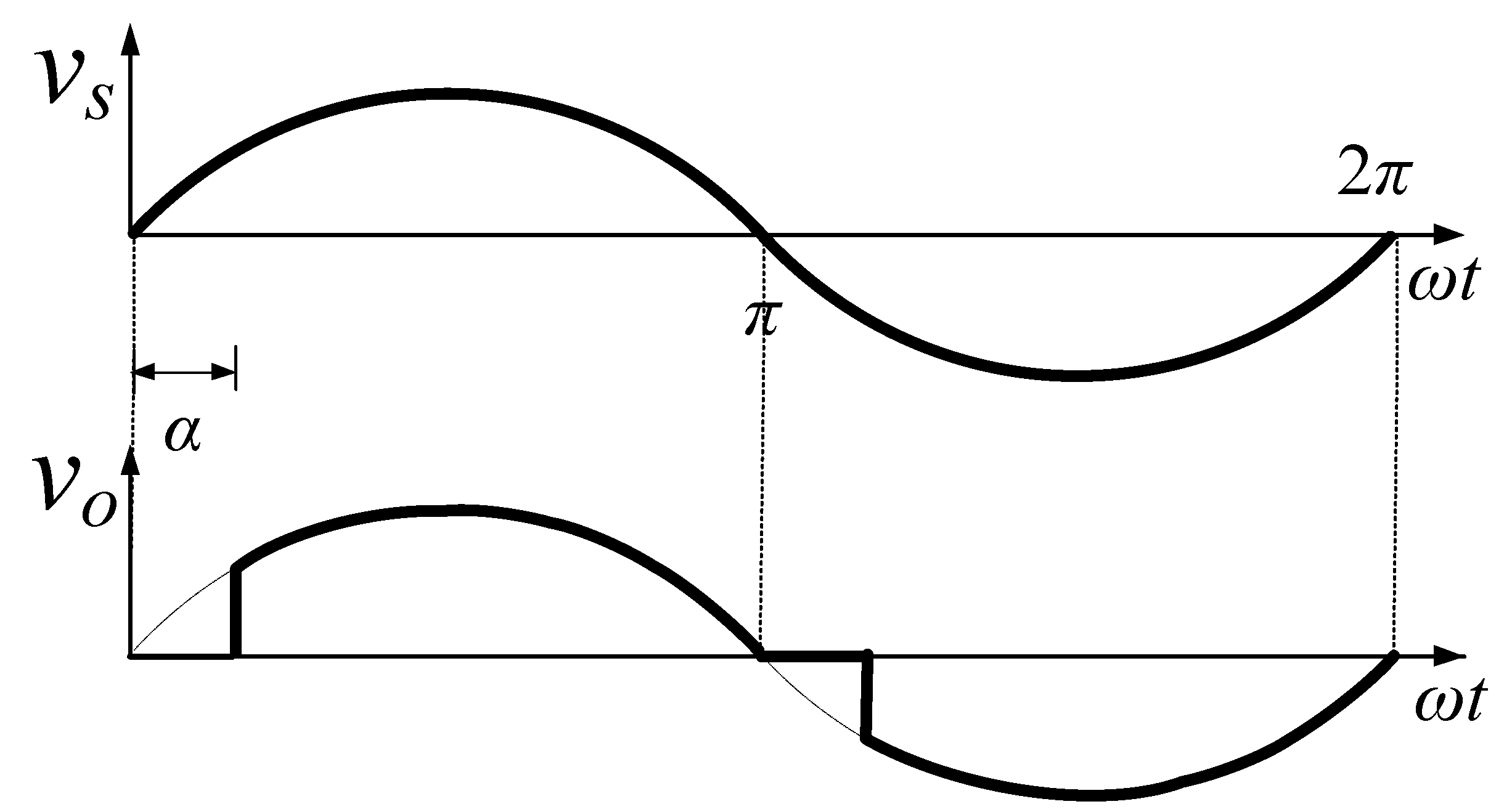
3.1.2. Voltage Regulation with Bipolar Voltage Control Scheme
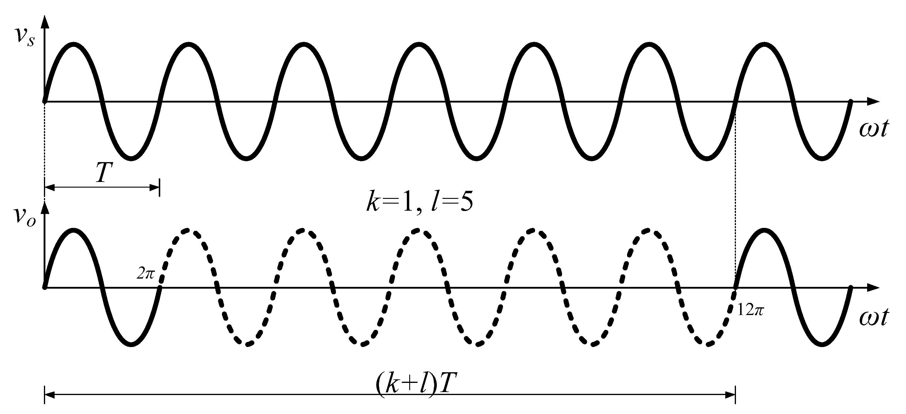
In this voltage control scheme, both half cycles of the input voltage are controlled (see Figure 3). That is accomplished by applying two gate pulses in one cycle of the input voltage. This is realized normally through the line commutated thyristor converters. Output RMS voltage is normally regulated through the firing delay control of the thyristors. There is no issue in the calculation of harmonics coefficients as the period of the output and input voltage waveform is equal to 2π.
The average value a0 of the output voltage is zero as the waveform is symmetric along the y-axis. This symmetry ensures the elimination of the even harmonics coefficients as computed analytically in Equations (8)–(11) to determine its power quality.
a n [ n 1 ]   =   { V m π ( n 1 ) [ 1 cos ( n α α ) ] V m π ( n + 1 ) [ 1 cos ( n α + α ) ] for   n   =   3 , 5 , 7 , 0 otherwise
b n [ n 1 ]   =   { V m π ( n + 1 ) sin ( n α + α ) V m π ( n 1 ) sin ( n α α ) for   n   =   3 , 5 , 7 , 0 otherwise
a n [ n = 1 ]   =   V m 2 π [ 1 + cos ( 2 α ) ]
b n [ n = 1 ]   =   V m π [ π α + 1 2 sin ( 2 α ) ]
Similarly, the closed-form of the instantaneous output voltage as the function of firing delay control ‘ α ’ is realized as
v o ( ω t ) =   V m π ( π α ) sin ( ω t ) V m 2 π [ cos ( ω t ) cos ( ω t 2 α ) ] + V m π ( n 1 ) [ cos ( n ω t ) cos ( n ω t n α + α ) ] V m π ( n + 1 ) [ cos ( n ω t ) cos ( n ω t n α α ) ] for   n   =   3 , 5 , 7 ,
The output voltage waveform has only odd harmonics as all other harmonics are suppressed due to the symmetrical nature of the waveform.

3.2. On-Off Control

This voltage control technique is employed to the load having high output time constant. In this control scheme, the load is connected to the input source for some integer cycles and disconnected for other integer cycles. The harmonics coefficients are computed through the pulse selective approach. In this approach, the harmonic coefficients of the output voltage are computed by considering its parent input voltage waveform. Figure 4 shows one on-cycle (k) and five off cycles (l).
The average value a0 is zero as the load is connected and disconnected for an integer number of cycles that makes this wave symmetrical along the y-axis. But, Figure 4 depicts that the periods of the output and input waveforms are unequal. To be specific, the period of the output voltage with a number of one ‘on-cycle’ and five ‘off-cycles’ is 12π, i.e., 2π(k + l). But the period of the input waveform is 2π. Here the output pulse is selected for six (k + l) cycles of the input for harmonics contents. The other Fourier coefficients based on PSA are realized in Equations (13)–(16).
a n [ n 6 ] = 2 12 π [ 0 π V m sin ( ω t ) cos ( n ω t 6 ) d ( ω t ) + π 2 π V m sin ( ω t ) cos ( n ω t 6 ) d ( ω t ) ] = 6 V m π ( 36 n 2 ) [ 1 cos ( 2 π n 6 ) ]
b n [ n 6 ] = 2 12 π [ 0 π V m sin ( ω t ) sin ( n ω t 6 ) d ( ω t ) + π 2 π V m sin ( ω t ) sin ( n ω t 6 ) d ( ω t ) ] = 6 V m π ( 36 n 2 ) sin ( 2 π n 6 )
The a6 and b6 are the required components (fundamental components/coefficients) of the output voltage and are separately computed as they become undefined at n = 6. That is to say
a 6 =   2 12 π [ 0 π V m sin ( ω t ) cos ( ω t ) d ( ω t ) + π 2 π V m sin ( ω t ) cos ( ω t ) d ( ω t ) ]   = 0
b 6 =   2 12 π [ 0 π V m sin ( ω t ) sin ( ω t ) d ( ω t ) + π 2 π V m sin ( ω t ) sin ( ω t ) d ( ω t ) ]   = V m 6
The amplitude of the harmonics and fundamental components start decreasing and increasing respectively by increasing the number of on-cycles. This characteristic is explored in Table 1 for various combinations of a number of ‘on’ and ‘off’ cycles.
The analysis of Table 1 gives the following generalized form.
a n [ n ( k + l ) ]   =   ( k + l ) V m π ( ( k + l ) 2 n 2 ) [ 1 cos ( 2 k π n ( k + l ) ) ]
b n [ n ( k + l ) ]   =   ( k + l ) V m π ( ( k + l ) 2 n 2 ) sin ( 2 k π n ( k + l ) )
b ( k + l )   =   k V m ( k + l ) a ( k + l ) = 0
The following general form of the output voltage is thus formulated as
v o ( ω t ) = k V m ( k + l ) sin ( ω t ) + V m π n = 1 , 2 , 3 n ( k + l ) ( k + l ) [ ( k + l ) 2 n 2 ] [ { 1 cos ( 2 π k n k + l ) } cos ( n ω t k + l ) { sin ( 2 π k n k + l ) sin ( n ω t k + l ) } ]

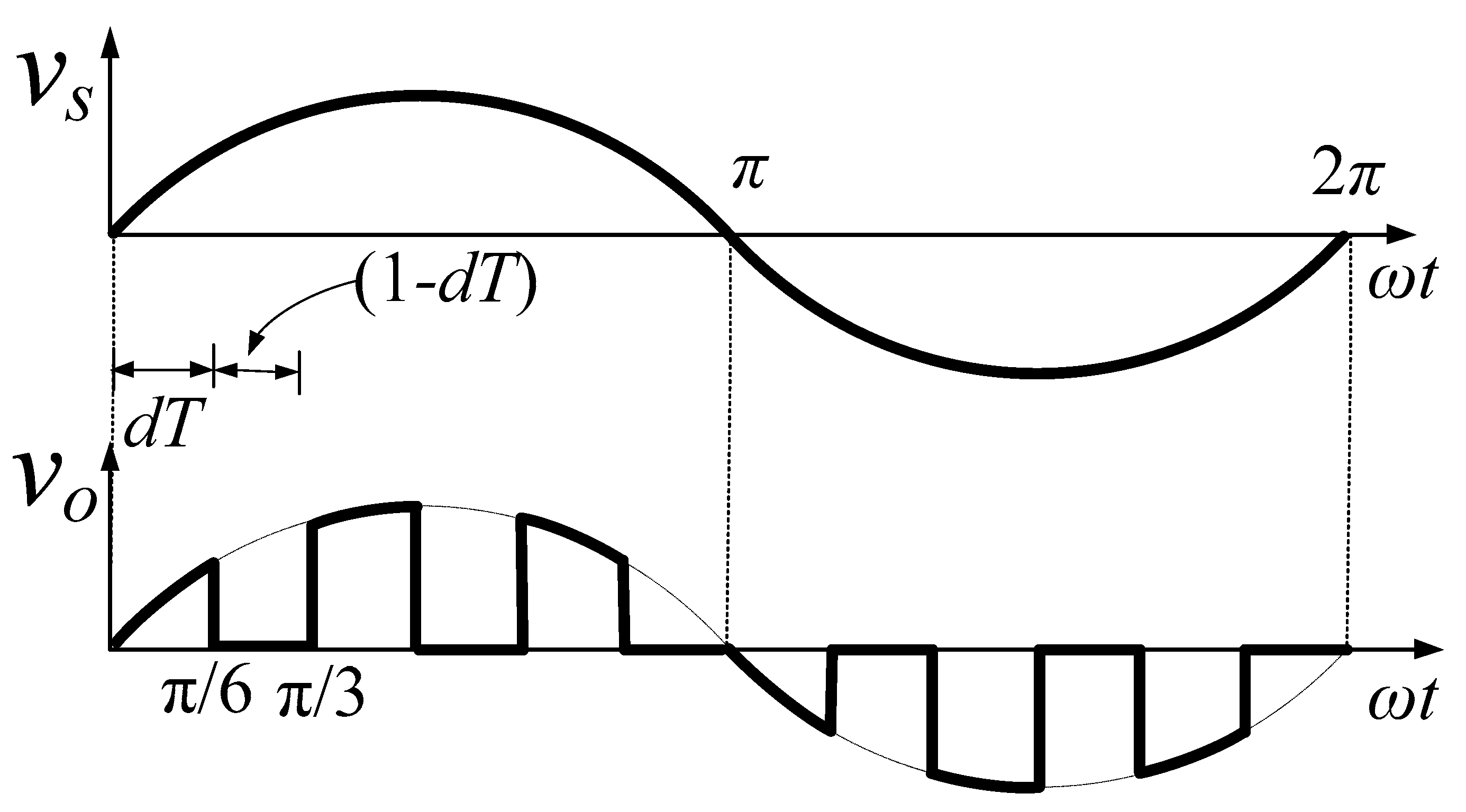
3.3. PWM Voltage Control

The use of phase-angle control and on-off control is restricted as they have low-frequency harmonics as their output voltages are obtained by operating the switching devices at low frequencies. The low-frequency harmonics are difficult to filter out. In this approach, the low-frequency harmonics are pushed to high frequency by increasing the switching frequency so that they can be easily filtered out. Here ‘dT’ is the intervals in which the instantaneous output voltage is equal to the instantaneous input voltage and for the ‘1 − dT’ interval, it is zero. The pulse on and off periods are equal and depend on the switching frequency of the controlled devices.
The power quality of the output voltage can be explored by computing the harmonics analytically through a pulse selective approach. In this approach, the instantaneous output voltage is decomposed into its parent’s sinusoidal waveform (see Figure 5). Based on this approach, the following harmonics coefficients are computed where the chopping frequency is six times the source frequency. Therefore, there are six sinusoidal pulses in one cycle of the input voltage. The harmonics coefficients of a six pulse waveform are analytically realized in Equations (21)–(24) by considering the turn on intervals of the PWM pulses.
a n ( n 1 )   =   2 2 π [ 0 π / 6 V m cos ( n ω t ) sin ( ω t ) + 2 π / 6 3 π / 6 V m cos ( n ω t ) sin ( ω t ) + 4 π / 6 5 π / 6 V m cos ( n ω t ) sin ( ω t ) + 6 π / 6 7 π / 6 V m cos ( n ω t ) sin ( ω t ) + 8 π / 6 9 π / 6 V m cos ( n ω t ) sin ( ω t ) + 10 π / 6 11 π / 6 V m cos ( n ω t ) sin ( ω t ) ]   = { V m π ( n 1 ) [ 3 cos ( π n 6 ) cos ( 2 π n 6 ) + sin ( π n 6 ) 3 sin ( 2 π n 6 ) + sin ( 3 π n 6 ) 1 ] + V m π ( n + 1 ) [ 3 cos ( π n 6 ) + cos ( 2 π n 6 ) + sin ( π n 6 ) 3 sin ( 2 π n 6 ) + sin ( 3 π n 6 ) + 1 ] for   n = 3 , 5 , 7 ,
b n ( n 1 )   =   2 2 π [ 0 π / 6 V m sin ( n ω t ) sin ( ω t ) + 2 π / 6 3 π / 6 V m sin ( n ω t ) sin ( ω t ) + 4 π / 6 5 π / 6 V m sin ( n ω t ) sin ( ω t ) + 6 π / 6 7 π / 6 V m sin ( n ω t ) sin ( ω t ) + 8 π / 6 9 π / 6 V m sin ( n ω t ) sin ( ω t ) + 10 π / 6 11 π / 6 V m sin ( n ω t ) sin ( ω t ) ] = 0
a n ( n = 1 )   =   2 2 π [ 0 π / 6 V m cos ( ω t ) sin ( ω t ) + 2 π / 6 3 π / 6 V m cos ( ω t ) sin ( ω t ) + 4 π / 6 5 π / 6 V m cos ( ω t ) sin ( ω t ) + 6 π / 6 7 π / 6 V m cos ( ω t ) sin ( ω t ) + 8 π / 6 9 π / 6 V m cos ( ω t ) sin ( ω t ) + 10 π / 6 11 π / 6 V m cos ( ω t ) sin ( ω t ) ] = 0
b n ( n = 1 )   =   2 2 π [ 0 π / 6 V m sin ( ω t ) sin ( ω t ) + 2 π / 6 3 π / 6 V m sin ( ω t ) sin ( ω t ) + 4 π / 6 5 π / 6 V m sin ( ω t ) sin ( ω t ) + 6 π / 6 7 π / 6 V m sin ( ω t ) sin ( ω t ) + 8 π / 6 9 π / 6 V m sin ( ω t ) sin ( ω t ) + 10 π / 6 11 π / 6 V m sin ( ω t ) sin ( ω t ) ] = V m 2
The following generalized form of the instantaneous output voltage for any pulse number is deduced from the analysis of Equations (21)–(24).
v o ( ω t ) =   V m 2 sin ( ω t )   + { 2 V m π ( n 1 ) k = 1 , 2 , 3 p 1 [ { ( 1 ) k + 1 cos ( k π n 2 p k π 2 p ) } + { ( 1 ) p cos ( π n 2 π 2 ) } 1 2 ] + 2 V m π ( n + 1 ) k = 1 , 2 , 3 p 1 [ { ( 1 ) k cos ( k π n 2 p + k π 2 p ) } + { ( 1 ) p cos ( π n 2 + π 2 ) } + 1 2 ] } cos ( n ω t )        
where ‘p’ is the number of pulses in each cycle of the input voltage. The symmetrical nature of the output waveform eliminates the dc (a0) and evens harmonics coefficients.

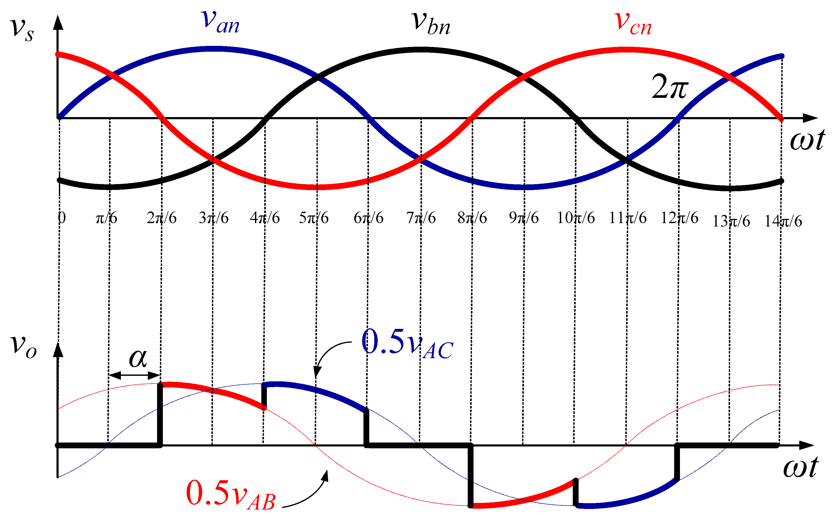
4. Three-Phase AC Voltage Controller

This AC voltage controller may also be used for speed regulation or soft starting of the heavy-duty three-phase AC motors. Figure 6 shows the waveform of the output phase voltage of a three-phase AC voltage controller with a firing delay of 30° or π/6.
It can be observed that the instantaneous value of one of the output phase voltages is ‘0.5 vAB’ during the interval from ωt = π/3 to 2π/3 and from ωt = 4π/3 to 5π/3. In the same way, it is ‘0.5 vAC’ during the interval from ωt = 2π/3 to π and from ωt = 5π/3 to 2π. The range of the firing delay during this voltage control mode is controlled from 30° (π/6) to 60° (2π/6). The instantaneous output voltage in this operating mode can be represented in generalized form as
v o ( ω t ) = { 1 2 v A B for π 6 + α ω t 3 π 6 + α and 7 π 6 + α ω t 9 π 6 + α 1 2 v A C for 3 π 6 + α ω t 5 π 6 + α and 9 π 6 + α ω t 11 π 6 + α
here
v A B 2 = 3 4 V m sin ( ω t ) + 3 4 cos ( ω t ) v A C 2 = 3 4 V m sin ( ω t ) 3 4 cos ( ω t )
Equations (27)–(30) are analytically developed through the pulse selective approach to analyze the harmonics coefficients of the phase voltage of a three-phase AC voltage controller. The average component (a0) is zero as the instantaneous output phase voltage has symmetric characteristics along the y-axis. The other harmonics are realized as
a n [ n 1 ] = 1 π [ ( π / 6 ) + α ( 3 π / 6 ) + α 3 V m 4 sin ( ω t ) cos ( n ω t ) d ( ω t ) + ( π / 6 ) + α ( 3 π / 6 ) + α 3 V m 4 cos ( ω t ) cos ( n ω t ) d ( ω t ) + ( 3 π / 6 ) + α ( 5 π / 6 ) + α 3 V m 4 sin ( ω t ) cos ( n ω t ) d ( ω t ) ( 3 π / 6 ) + α ( 5 π / 6 ) + α 3 V m 4 cos ( ω t ) cos ( n ω t ) d ( ω t ) + ( 7 π / 6 ) + α ( 9 π / 6 ) + α 3 V m 4 sin ( ω t ) cos ( n ω t ) d ( ω t ) + ( 7 π / 6 ) + α ( 9 π / 6 ) + α 3 V m 4 cos ( ω t ) cos ( n ω t ) d ( ω t ) + ( 9 π / 6 ) + α ( 11 π / 6 ) + α 3 V m 4 sin ( ω t ) cos ( n ω t ) d ( ω t ) ( 9 π / 6 ) + α ( 11 π / 6 ) + α 3 V m 4 cos ( ω t ) cos ( n ω t ) d ( ω t ) ]   = 3 V m 2 π ( n 1 ) [ sin ( n π 6 ) 3 cos ( n π 6 ) + sin ( n π 2 ) ] sin ( n α α ) 3 V m 2 π ( n + 1 ) [ sin ( n π 6 ) + 3 cos ( n π 6 ) + sin ( n π 2 ) ] sin ( n α + α )
b n [ n 1 ] = 1 π [ ( π / 6 ) + α ( 3 π / 6 ) + α 3 V m 4 sin ( ω t ) sin ( n ω t ) d ( ω t ) + ( π / 6 ) + α ( 3 π / 6 ) + α 3 V m 4 cos ( ω t ) sin ( n ω t ) d ( ω t ) + ( 3 π / 6 ) + α ( 5 π / 6 ) + α 3 V m 4 sin ( ω t ) sin ( n ω t ) d ( ω t ) ( 3 π / 6 ) + α ( 5 π / 6 ) + α 3 V m 4 cos ( ω t ) sin ( n ω t ) d ( ω t ) + ( 7 π / 6 ) + α ( 9 π / 6 ) + α 3 V m 4 sin ( ω t ) sin ( n ω t ) d ( ω t ) + ( 7 π / 6 ) + α ( 9 π / 6 ) + α 3 V m 4 cos ( ω t ) sin ( n ω t ) d ( ω t ) + ( 9 π / 6 ) + α ( 11 π / 6 ) + α 3 V m 4 sin ( ω t ) sin ( n ω t ) d ( ω t ) ( 9 π / 6 ) + α ( 11 π / 6 ) + α 3 V m 4 cos ( ω t ) sin ( n ω t ) d ( ω t ) ]   = 3 V m 2 π ( n 1 ) [ sin ( n π 6 ) 3 cos ( n π 6 ) + sin ( n π 2 ) ] cos ( n α α ) + 3 V m 2 π ( n + 1 ) [ sin ( n π 6 ) + 3 cos ( n π 6 ) + sin ( n π 2 ) ] cos ( n α + α )
The harmonic coefficients for the fundamental component are separately computed in Equations (29) and (30).
b n [ n = 1 ] = 1 π [ ( π / 6 ) + α ( 3 π / 6 ) + α 3 V m 4 sin ( ω t ) sin ( ω t ) d ( ω t ) + ( π / 6 ) + α ( 3 π / 6 ) + α 3 V m 4 cos ( ω t ) sin ( ω t ) d ( ω t ) + ( 3 π / 6 ) + α ( 5 π / 6 ) + α 3 V m 4 sin ( ω t ) sin ( ω t ) d ( ω t ) ( 3 π / 6 ) + α ( 5 π / 6 ) + α 3 V m 4 cos ( ω t ) sin ( ω t ) d ( ω t ) + ( 7 π / 6 ) + α ( 9 π / 6 ) + α 3 V m 4 sin ( ω t ) sin ( ω t ) d ( ω t ) + ( 7 π / 6 ) + α ( 9 π / 6 ) + α 3 V m 4 cos ( ω t ) sin ( ω t ) d ( ω t ) + ( 9 π / 6 ) + α ( 11 π / 6 ) + α 3 V m 4 sin ( ω t ) sin ( ω t ) d ( ω t ) ( 9 π / 6 ) + α ( 11 π / 6 ) + α 3 V m 4 cos ( ω t ) sin ( ω t ) d ( ω t ) ]   = V m 2 + 3 3 V m 4 π cos ( 2 α )      
a n [ n = 1 ] = 1 π [ ( π / 6 ) + α ( 3 π / 6 ) + α 3 V m 4 sin ( ω t ) sin ( ω t ) d ( ω t ) + ( π / 6 ) + α ( 3 π / 6 ) + α 3 V m 4 cos ( ω t ) sin ( ω t ) d ( ω t ) + ( 3 π / 6 ) + α ( 5 π / 6 ) + α 3 V m 4 sin ( ω t ) sin ( ω t ) d ( ω t ) ( 3 π / 6 ) + α ( 5 π / 6 ) + α 3 V m 4 cos ( ω t ) sin ( ω t ) d ( ω t ) + ( 7 π / 6 ) + α ( 9 π / 6 ) + α 3 V m 4 sin ( ω t ) sin ( ω t ) d ( ω t ) + ( 7 π / 6 ) + α ( 9 π / 6 ) + α 3 V m 4 cos ( ω t ) sin ( ω t ) d ( ω t ) + ( 9 π / 6 ) + α ( 11 π / 6 ) + α 3 V m 4 sin ( ω t ) sin ( ω t ) d ( ω t ) ( 9 π / 6 ) + α ( 11 π / 6 ) + α 3 V m 4 cos ( ω t ) sin ( ω t ) d ( ω t ) ]   = 3 3 V m 4 π sin ( 2 α )

5. Single-Phase Direct Frequency Controller

Single-phase direct AC-AC converters may also be employed to govern the output frequency in discrete steps. In these power converting topologies, the frequency at the output may be increased and decreased with respect to source frequency. Here the frequency step-up outputs are considered to explore the use of the pulse selective approach for their power quality concerns. Figure 7a,b depicts the outputs having frequencies two and three times the input frequency respectively.
The period of the required component of output in Figure 7a is equal to the period of the waveform as its average value during the output periods is zero. The harmonic coefficients of this output are calculated in Equations (31) and (32) by selecting the output pulse for the ‘π’ period.
a n   = 1 π [ 0 π / 2 2 V m cos ( 2 n ω t ) sin ( ω t ) d ( ω t ) π / 2 π 2 V m cos ( 2 n ω t ) sin ( ω t ) d ( ω t ) ] = 0
b n = 1 π [ 0 π / 2 2 V m sin ( 2 n ω t ) sin ( ω t ) d ( ω t ) π / 2 π 2 V m sin ( 2 n ω t ) sin ( ω t ) d ( ω t ) ] = 2 V m π ( 2 n 1 ) cos ( n π ) 2 V m π ( 2 n + 1 ) cos ( n π )
These coefficients can also be formulated by considering for ‘2π’ period as in Equations (33) and (34).
a n   = 1 2 π [ 0 π / 2 2 V m cos ( n ω t ) sin ( ω t ) d ( ω t ) π / 2 3 π / 2 2 V m cos ( n ω t ) sin ( ω t ) d ( ω t ) + 3 π / 2 2 π 2 V m cos ( n ω t ) sin ( ω t ) d ( ω t ) ] = 0
b n = 1 2 π [ 0 π / 2 2 V m cos ( n ω t ) sin ( ω t ) d ( ω t ) π / 2 3 π / 2 2 V m cos ( n ω t ) sin ( ω t ) d ( ω t ) + 3 π / 2 2 π 2 V m cos ( n ω t ) sin ( ω t ) d ( ω t ) ] = { 2 V m π ( n 1 ) cos ( n π 2 ) 2 V m π ( n + 1 ) cos ( n π 2 )         for     n =   2 , 4 , 6 ,
The output waveform of Figure 7b has a non-zero average value in the period of the required output voltage component as its output pulses are asymmetric along the y-axis. It means that the period of the required component is not the same as the period of the output pulses. Power quality analysis with the period of the output pulse leads to incorrect results. To tackle this issue, select the period of the waveform at which the average value of the waveform becomes zero and it is observed to be ‘2π’. The harmonic coefficients depending upon this period are evaluated in Equations (35) and (36).
a n   = 1 2 π [ 0 π / 3 2 V m cos ( n ω t ) sin ( ω t ) d ( ω t ) π / 3 2 π / 3 2 V m cos ( n ω t ) sin ( ω t ) d ( ω t ) + 2 π / 3 4 π / 3 2 V m cos ( n ω t ) sin ( ω t ) d ( ω t ) 4 π / 3 5 π / 3 2 V m cos ( n ω t ) sin ( ω t ) d ( ω t ) + 5 π / 3 2 π 2 V m cos ( n ω t ) sin ( ω t ) d ( ω t ) ] = 0
b n = 1 2 π [ 0 π / 3 2 V m sin ( n ω t ) sin ( ω t ) d ( ω t ) π / 3 2 π / 3 2 V m sin ( n ω t ) sin ( ω t ) d ( ω t ) + 2 π / 3 4 π / 3 2 V m sin ( n ω t ) sin ( ω t ) d ( ω t ) 4 π / 3 5 π / 3 2 V m sin ( n ω t ) sin ( ω t ) d ( ω t ) + 5 π / 3 2 π 2 V m sin ( n ω t ) sin ( ω t ) d ( ω t ) ] = { 2 V m π ( n + 1 ) [ sin ( n π 3 ) + 3 cos ( n π 3 ) ] + 2 V m π ( n 1 ) [ sin ( n π 3 ) 3 cos ( n π 3 ) ] for   n = 3 , 5 , 7 ,
In the same way, the harmonic coefficients for the output frequency of 25, 100, 150, and 200 Hz with 50 Hz input frequency for an output pulse period of ‘4π’ exercised in [26] are demonstrated in Equations (37)–(40).
a n = 0 , b n = { 8 V m π ( 4 n 2 ) sin ( n π 2 )   for   n = 1 , 3 , 5 , 0 , otherwise
a n = 0 , b n = { 4 V m π ( n 2 ) { sin ( n π 4 2 π 4 ) + 1 2 sin ( 2 n π 2 ) } 4 V m π ( n + 2 ) { sin ( n π 4 + 2 π 4 ) + 1 2 sin ( 2 n π 2 ) } , for   n = 4 , 8 , 12 , 16 , 0 , otherwise
a n = 0 b n = { 4 V m π ( n 2 ) { sin ( n π 6 2 π 6 ) sin ( 2 n π 6 4 π 6 ) + 1 2 sin ( 4 n π 2 ) } 4 V m π ( n + 2 ) { sin ( n π 6 + 2 π 6 ) sin ( 2 n π 6 + 4 π 6 ) + 1 2 sin ( 4 n π 2 ) } , for   n = 2 , 6 , 10 , 14 , 0 , otherwise
a n = 0 b n = { 4 V m π ( n 2 ) { sin ( n π 8 2 π 8 ) sin ( 2 n π 8 4 π 8 ) + sin ( 3 n π 8 6 π 8 ) + 1 2 sin ( 6 n π 2 ) } 4 V m π ( n + 2 ) { sin ( n π 8 + 2 π 8 ) sin ( 2 n π 8 + 4 π 8 ) + sin ( 3 n π 8 + 6 π 8 ) + 1 2 sin ( 6 n π 2 ) } , for   n = 4 , 8 , 12 , 16 , 0 , otherwise
The harmonic coefficients of the output frequency of 100 Hz are evaluated in Equations (31)–(34) and (38) for three output periods i.e., by selecting the actual period, two and four times the actual period. Their validity can be viewed for the required voltage component (100 Hz component) by putting n = 1, 2, and 4 in Equations (32), (34), and (38) respectively. The output RMS voltage (Vo2) in all three cases is depicted in Equation (41). In the same way, with the use of the computed harmonic coefficients in Equations (36) and (39) for the output frequency of 150 Hz, the RMS output voltage (Vo3) is evaluated in Equation (42) by putting n = 1 and 2 respectively.
V o 2 = 4 2 V m 3 π
V o 3 = 3 3 V m 2 2 π

6. Validation of the Generated Harmonics

The generated harmonics are verified through the simulation, practical and analytical results.

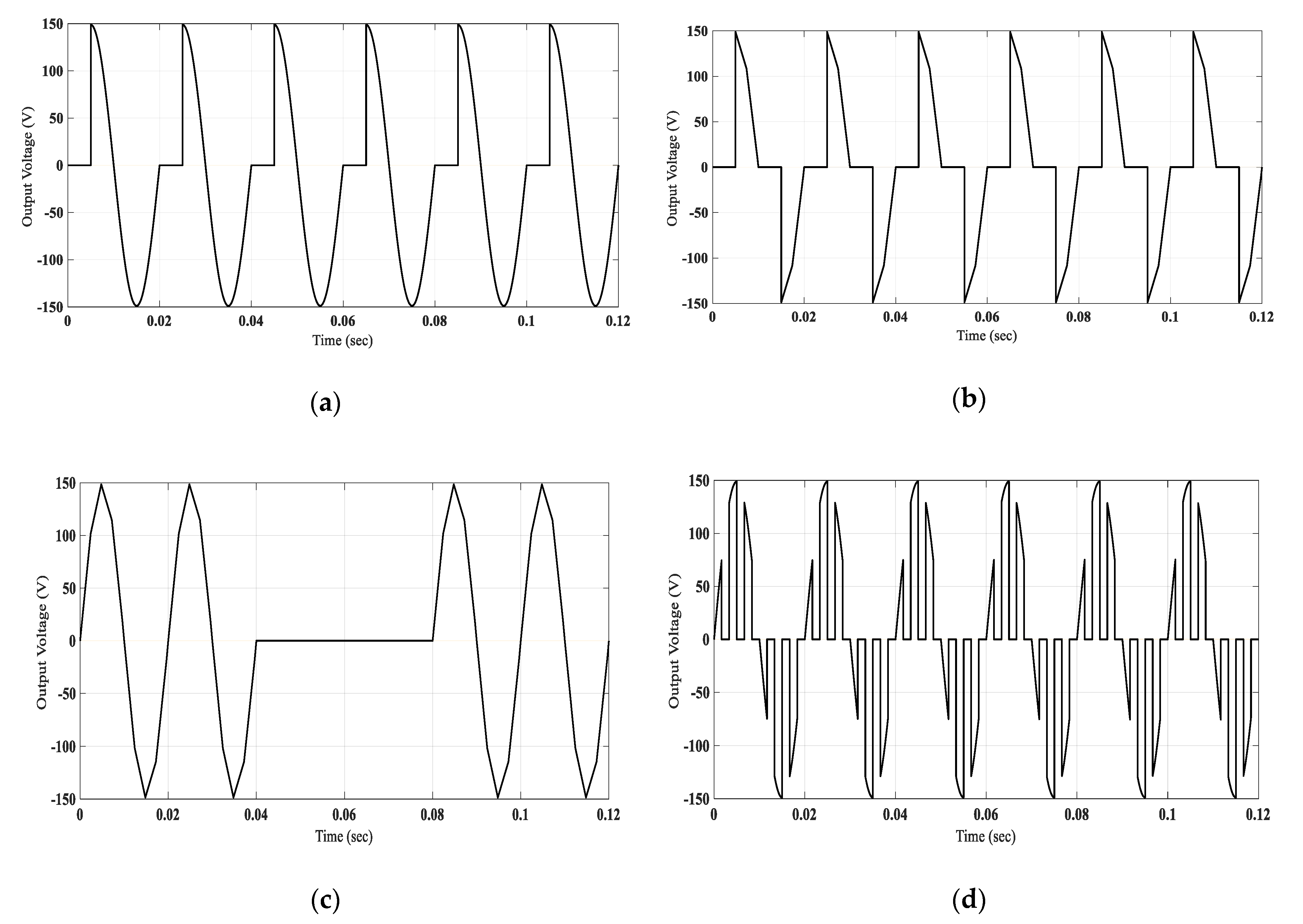
6.1. Validation through Simulation and Analytical Results

The Simulink-based environment is used to validate the computed harmonics coefficients for various output voltage control schemes. Figure 8 shows the output voltage waveforms realized with phase-angle, on-off cycle, and PWM control. The output voltage waveform (see Figure 8a) is simulated with a firing-delay of π / 2 . With this control, the input voltage at the output is chopped from ‘0′ to ‘ π / 2 ’, which only generates a DC component and even and odd harmonics as depicted in Table 2. The DC component is negative as the area under the negative half cycle is greater than its positive half cycle area.
The output voltage waveform (see Figure 8b) is simulated with a firing-delay of π / 2 . With this control, the input voltage at the output is chopped from ‘0′ to ‘ π / 2 ’ and from ‘ π ’ to ‘ 3 π / 2 . This control generates low-frequency harmonics as the switching frequency is the same as that of the input source. These generated harmonics are verified from the simulated and mathematical results of Table 3 with a firing delay control of π / 2 . Here it can be observed that the maximum value of the voltage fundamental component, third, fifth, seventh, ninth, and eleventh harmonics are approximately 90 V, 48 V, 16 V, 16 V, 10 V, and 10 V, respectively with a 150 V peak input voltage.
As already remarked, the on-off cycle control is another voltage control technique used to govern the load voltage’s RMS value. This control scheme is also employed at a low switching frequency that results in the generation of low-frequency harmonics. The output voltage waveform of Figure 8c is obtained with an equal (two) number of ‘on’ and ‘off’ cycles. The generated harmonics of this output voltage waveform are tabulated in Table 4. These harmonics are also verified from the mathematically-computed results.
The generated harmonics with phase-angle or on-off cycle control cannot be moved at high frequency as their switching frequencies cannot be increased. This problem is tackled with PWM control. Here, the amplitude of the output voltage is controlled through the PWM control, and the frequency of the harmonics is governed through the switching frequency. Figure 8d shows the output voltage waveform obtained with PWM control having a 50% pulse width and switching frequency six times (300 Hz) as that of the input (50 Hz). This control shifts the harmonics at switching frequency and their integer multiple, as can be viewed from the results of the harmonics of Table 5. It can be observed from Table 5 that harmonics are shifted to 300 and 900 Hz.
The simulation results validate the mathematical formulation of Equations (7), (12), (20), and (25) developed for phase-angle, on-off cycle, and PWM control, respectively.
Figure 9a depicts the output phase voltage of a three-phase AC voltage controller. It can be observed that this output voltage waveform is almost symmetric along the y-axis in one period, so its simulated harmonics are approximately matched to the computed values as tabulated in Table 6. Now if the firing delay is changed from 60° to 90° to decrease the output RMS voltage, then the output voltage waveform becomes asymmetric along the y-axis in one period as shown in Figure 9b. This output voltage contains the DC component as well as even and odd harmonics. So, this leads to inaccurate results as can be viewed from the results of Table 7. Now if the wave starting time is adjusted in the Simulink plot as depicted in Figure 9c to get symmetry along the y-axis in one period of the waveform, then it improves the harmonic amplitude result but this adds a severe error in their phase angles as can be seen from the values in Table 8. On the other hand, there are no such issues in the power quality concerns that are based on the computed values.

6.2. Validation through Practical Results

No a new dedicated practical set-up is developed for the practical analysis of the power quality concerns. The practical results for power quality analysis are documented with the help of a practical set-up of our proposed power converting topologies reported in [25,26]. The plots of Figure 10 are obtained with the practical set-up of [25] by synchronizing the gating signals with input source voltage by applying the output of the zero-detecting circuit to the signal generator (STM controller) in the form of an interrupt. In the same way, the practical outputs presented in Figure 11 are obtained with the help of the practical set-up presented in [26]. These practical set-ups are developed with high switching MOSFETs (IRF840), diodes (RGHG3060), transistors driving circuits (EXB840), isolated DC supplies, and passives components.
Figure 10 demonstrates the practically recorded results of the output voltage and their FFTs for various switching control schemes. Figure 10a–d depicts the output voltage waveform of phase-angle with unipolar and bipolar, on-off cycle, and PWM voltage control, respectively. Their FFT results show the RMS value of the voltage fundamental components and some dominant harmonics. The practically obtained FFT of Figure 10a depicts the output voltage of the AC voltage controller realized with unipolar voltage control scheme has a DC component, and all even and odd harmonics. The FFT of Figure 10b shows that all even harmonics and DC components are suppressed from the output with the help of a bipolar voltage control scheme. The FFT plot of on-off control shown in Figure 10c depicts the dominant low-frequency harmonics. The shifting of low-frequency harmonics to high frequencies can be viewed from Figure 10d which is achieved by increasing the switching frequency.
The harmonics in the output voltage with PWM control can be easily suppressed with a low pass filter like other voltage control techniques as the generated harmonics with PWM control can be moved to high frequencies (switching frequencies) by increasing the switching frequencies. Figure 11 shows the output voltage and its FFT if the PWM output is passed through a low pass filter.
Similarly, the power quality analysis of the output voltage in variable frequency operation in [26] is explored by comparing the mathematical results with the simulation results. The output voltage waveforms for the output frequency of 25, 100, 150, and 200 Hz with their FFT results are plotted in Figure 12.
Table 9 compares the RMS values of the voltage fundamental components obtained from the mathematically formulated equation, measured results from the Simulink-based platform, and measured results from the practically plotted FFTs for the peak input voltage of 150 V.
Comparing the results of Table 2, Table 3, Table 4, Table 5, Table 6, Table 7, Table 8 and Table 9 depicts the effectiveness of the proposed analytical approach to compute the harmonics content of the various output of the direct AC-to-AC converters.

7. Conclusions

This research analytically analyzes the power quality of the output voltage in direct AC-AC power converters. The regulation in the output RMS voltage is accomplished through various voltage control techniques such as phase-delay control, on-off cycle control, and PWM control. Each voltage control scheme has a distinctive harmonic profile. In the same manner, the regulation of the output frequency also has a variation in harmonic contents. Therefore, an analytical pulse selective approach is employed to view the harmonic contents. Based on this analysis, the Fourier series of the output voltage for various voltage control schemes and in variable frequency operation is mathematically formulated. Their validity is proved through the simulation results obtained from the Simulink-based environment. Practically recorded FFT also supports the computed and simulated results.

Author Contributions

Conceptualization, N.A. and G.A.; Data curation, G.A. and R.A.; Formal analysis, N.A. and R.A.; Funding acquisition, R.A., H.J., N.A., and G.A.; Investigation, G.A. and H.J.; Methodology, N.A. and G.A.; Supervision, G.A.; Visualization, H.J.; Writing—original draft, N.A. and G.A.; Writing—review and editing, G.A., R.A., and H.J. All authors have read and agreed to the published version of the manuscript.

Funding

This research received no external funding.

Institutional Review Board Statement

Not applicable.

Informed Consent Statement

Not applicable.

Data Availability Statement

Not applicable.

Conflicts of Interest

The authors declare no conflict of interest.

References

  1. Sanjan, P.S.; Gowtham, N.; Bhaskar, M.S.; Subramaniam, U.; Almakhles, D.; Padmanaban, S.; Yamini, N.G. Enhancement of Power Quality in Domestic Loads Using Harmonic Filters. IEEE Access 2020, 8, 197730–197744. [Google Scholar] [CrossRef]
  2. Mazzanti, G.; Diban, B.; Chiodo, E.; de Falco, P.; di Noia, L.P. Forecasting the Reliability of Components Subjected to Harmonics Generated by Power Electronic Converters. Electronics 2020, 9, 1266. [Google Scholar] [CrossRef]
  3. Kefalas, T.D.; Kladas, A.G. Harmonic Impact on Distribution Transformer No-Load Loss. IEEE Trans. Ind. Electron. 2010, 57, 193–200. [Google Scholar] [CrossRef]
  4. Kumar, D.; Zare, F. Harmonic Analysis of Grid Connected Power Electronic Systems in Low Voltage Distribution Networks. IEEE J. Emerg. Sel. Top. Power Electron. 2016, 4, 70–79. [Google Scholar] [CrossRef]
  5. Zare, F.; Soltani, H.; Kumar, D.; Davari, P.; Delpino, H.A.M.; Blaabjerg, F. Harmonic Emissions of Three-Phase Diode Rectifiers in Distribution Networks. IEEE Access 2017, 5, 2819–2833. [Google Scholar] [CrossRef]
  6. Das, J.C. Passive filters—Potentialities and limitations. IEEE Trans. Ind. Appl. 2004, 40, 232–241. [Google Scholar] [CrossRef]
  7. Wang, X.; Blaabjerg, F.; Wu, W. Modeling and Analysis of Harmonic Stability in an AC Power-Electronics-Based Power System. IEEE Trans. Power Electron. 2014, 29, 6421–6432. [Google Scholar] [CrossRef]
  8. Quevedo, D.E.; Aguilera, R.P.; Perez, M.A.; Cortes, P.; Lizana, R. Model Predictive Control of an AFE Rectifier with Dynamic References. IEEE Trans. Power Electron. 2012, 27, 3128–3136. [Google Scholar] [CrossRef]
  9. Rahmani, S.; Mendalek, N.; Al-Haddad, K. Experimental Design of a Nonlinear Control Technique for Three-Phase Shunt Active Power Filter. IEEE Trans. Ind. Electron. 2010, 57, 3364–3375. [Google Scholar] [CrossRef]
  10. Ribeiro, R.L.d.; de Azevedo, C.C.; de Sousa, R.M. A Robust Adaptive Control Strategy of Active Power Filters for Power-Factor Correction, Harmonic Compensation, and Balancing of Nonlinear Loads. IEEE Trans. Ind. Electron. 2012, 27, 718–730. [Google Scholar]
  11. Wang, X.; Pang, Y.; Loh, P.C.; Blaabjerg, F. A Series-LC-Filtered Active Damper with Grid Disturbance Rejection for AC Power-Electronics-Based Power Systems. IEEE Trans. Ind. Power Electron. 2015, 30, 4037–4041. [Google Scholar] [CrossRef]
  12. Zhao, N.; Wang, G.; Ding, D.; Zhang, G.; Xu, D. Impedance Based Stabilization Control Method for Reduced DC-Link Capacitance IPMSM Drives. IEEE Trans. Ind. Power Electron. 2019, 34, 9879–9890. [Google Scholar] [CrossRef]
  13. Meng, F.; Yang, W.; Yang, S. Effect of Voltage Transformation Ratio on the Kilovoltampere Rating of Delta-Connected Autotransformer for 12-Pulse Rectifier System. IEEE Trans. Ind. Electron. 2013, 60, 3579–3588. [Google Scholar] [CrossRef]
  14. Setlak, L.; Kowalik, R. Examination of multi-pulse rectifiers of PES systems used on airplanes compliant with the concept of electrified aircraft. Appl. Sci. 2019, 9, 1520. [Google Scholar] [CrossRef] [Green Version]
  15. Iwaszkiewicz, J.; Mysiak, P. Supply System for Three-Level Inverters Using Multi-Pulse Rectifiers with Coupled Reactors. Energies 2019, 12, 3385. [Google Scholar] [CrossRef] [Green Version]
  16. Yuan, D.; Wang, S.; Liu, Y. Dynamic Phasor Modeling of Various Multipulse Rectifiers and a VSI Fed by 18-Pulse Asymmetrical Autotransformer Rectifier Unit for Fast Transient Analysis. IEEE Access 2020, 8, 43145–43155. [Google Scholar] [CrossRef]
  17. Ashraf, N.; Izhar, T.; Abbas, G.; Yasin, A.R.; Kashif, A.R. Power quality analysis of a three-phase ac-to-dc controlled converter. In Proceedings of the 2017 International Conference on Electrical Engineering (ICEE), Lahore, Pakista, 2–4 March 2017; pp. 1–6. [Google Scholar]
  18. Siami, M.; Khaburi, D.A.; Rivera, M.; Rodríguez, J. An Experimental Evaluation of Predictive Current Control and Predictive Torque Control for a PMSM Fed by a Matrix Converter. IEEE Trans. Ind. Power Electron. 2017, 64, 8459–8471. [Google Scholar] [CrossRef]
  19. Elrayyah, A.; Safayet, Y.; Sozer, I.H.; Elbuluk, M. Efficient harmonic and phase estimator for single-phase grid-connected renewable energy systems. IEEE Trans. Ind. Power Appl. 2013, 1, 50. [Google Scholar] [CrossRef]
  20. Baradarani, F.; Zadeh, M.R.D.; Zamani, M.A. A phase-angle estimation method for synchronization of grid-connected power-electronic converters. IEEE Trans. Power Deliv. 2014, 30, 2. [Google Scholar] [CrossRef]
  21. Hansen, S.; Nielsen, P.; Blaabjerg, F. Harmonic cancellation by mixing nonlinear single-phase and three-phase loads. IEEE Trans. Ind. Appl. 2000, 36, 152–159. [Google Scholar] [CrossRef]
  22. Sharifi, S.; Monfared, M.; Babaei, M.; Pourfaraj, A. Highly Efficient Single-Phase Buck–Boost Variable-Frequency AC–AC Converter with Inherent Commutation Capability. IEEE Trans. Ind. Electron. 2020, 67, 3640–3649. [Google Scholar] [CrossRef]
  23. Ashraf, N.; Izhar, T.; Abbas, G.; Balas, V.E.; Balas, M.M.; Lin, T.; Asad, M.U.; Farooq, U.; Gu, J. A Single-Phase Buck and Boost AC-to-AC Converter with Bipolar Voltage Gain: Analysis, Design, and Implementation. Energies 2019, 12, 1376. [Google Scholar] [CrossRef] [Green Version]
  24. Ashraf, N.; Izhar, T.; Abbas, G.; Awan, A.B.; Farooq, U.; Balas, V.E. A New Single-Phase AC Voltage Converter with Voltage Buck Characteristics for Grid Voltage Compensation. IEEE Access 2020, 8, 48886–48903. [Google Scholar] [CrossRef]
  25. Ashraf, N.; Izhar, T.; Abbas, G.; Awan, A.B.; Alghamdi, A.S.; Abo-Khalil, A.G.; Sayed, K.; Farooq, U.; Balas, V.E. A New Single-Phase Direct Frequency Controller Having Reduced Switching Count without Zero-Crossing Detector for Induction Heating System. Electronics 2020, 9, 430. [Google Scholar] [CrossRef] [Green Version]
  26. Ashraf, N.; Izhar, T.; Abbas, G. A Single-Phase Buck-Boost Matrix Converter with Low Switching Stresses. Math. Probl. Eng. 2019, 2019, 6893546. [Google Scholar] [CrossRef]
  27. Xiuyun, W.; Wei, T.; Wang, R.; Hu, Y.; Liu, S. A Novel Carrier-Based PWM without Narrow Pulses Applying to High-Frequency Link Matrix Converter. IEEE Access 2020, 8, 157654–157662. [Google Scholar]
  28. Shi, N.; Zhang, X.; An, S.B.; Yan, Y.; Xia, C.L. Harmonic suppression modulation strategy for ultra-sparse matrix converter. IET Power Electron. 2016, 9, 589–599. [Google Scholar] [CrossRef]
  29. Dinh, T.N.; Dzung, P.Q. Space vector modulation for an indirect matrix converter with improved input power factor. Energies 2017, 10, 588. [Google Scholar]
  30. Qi, C.; Chen, X.; Qiu, Y. Carrier-Based Randomized Pulse Position Modulation of an Indirect Matrix Converter for Attenuating the Harmonic Peaks. IEEE Trans. Power Electron. 2013, 28, 3539–3548. [Google Scholar] [CrossRef]
  31. Wang, H. Topology and Modulation Scheme of a Three-Level Third-Harmonic Injection Indirect Matrix Converter. IEEE Trans. Ind. Electron. 2017, 64, 7612–7622. [Google Scholar] [CrossRef]
  32. Moynihan, F.J.; Egan, M.G.; Murphy, J.M.D. Theoretical spectra of space-vector-modulated waveforms. IEEE Proc. Electr. Power Appl. 1998, 145, 17–24. [Google Scholar] [CrossRef]
  33. You, K.; Xiao, D.; Rahman, M.F.; Uddin, M.N. Applying Reduced General Direct Space Vector Modulation Approach of AC–AC Matrix Converter Theory to Achieve Direct Power Factor Controlled Three-Phase AC–DC Matrix Rectifier. IEEE Trans. Ind. Electron. 2014, 50, 2243–2257. [Google Scholar] [CrossRef]
  34. Lian, K.L.; Perkins, B.K.; Lehn, P.W. Harmonic analysis of a three-phase diode bridge rectifier based on sampled-data model. IEEE Trans. Power Deliv. 2008, 23, 2. [Google Scholar] [CrossRef]
  35. Kwon, J.B.; Wang, X.; Blaabjerg, F.; Bak, C.L.; Sularea, V.S.; Busca, C. Harmonic interaction analysis in a grid-connected converter using harmonic state-space (HSS) modeling. IEEE Trans. Power Electron. 2016, 32, 9. [Google Scholar]
  36. Freitas, L.C.G.D.; Simões, M.G.; Canesin, C.A.; Freitas, L.C.D. Performance evaluation of a novel hybrid multipulse rectifier for utility interface of power electronic converters. IEEE Trans. Ind. Electron. 2007, 54, 6. [Google Scholar]
Figure 1. Flow chart of the pulse selective approach (PSA).
Applsci 11 00538 g001
Figure 2. Output RMS voltage control through unipolar phase-angle control.
Applsci 11 00538 g002
Figure 3. Output RMS voltage control through bipolar phase-angle control.
Applsci 11 00538 g003
Figure 4. Output RMS voltage control through on-off cycle control.
Applsci 11 00538 g004
Figure 5. Output RMS voltage control through the pulse-width modulation (PWM) control.
Applsci 11 00538 g005
Figure 6. Output RMS voltage control of three-phase AC voltage controller.
Applsci 11 00538 g006
Figure 7. Variable frequency outputs with respect to input (a) double frequency and (b) triple frequency.
Applsci 11 00538 g007
Figure 8. Simulation waveforms of the output voltage: (a) phase-angle unipolar control; (b) phase-angle bipolar control; (c) on-off cycle control; (d) PWM control.
Applsci 11 00538 g008
Figure 9. The output voltage waveform of one phase of a three-phase AC voltage controller with a firing delay of (a) 60°, (b) 90°, and (c) 90° with appropriate wave shifting.
Applsci 11 00538 g009aApplsci 11 00538 g009b
Figure 10. Practical waveform of the output voltage: (a) phase-angle with unipolar control; (b) phase-angle with bipolar control (c) on-off cycle control; (d) PWM control.
Applsci 11 00538 g010
Figure 11. The practical waveform of the output voltage with PWM control and a low pass filter.
Applsci 11 00538 g011
Figure 12. Practical waveform of the output voltage with output frequency: (a) 25 Hz; (b) 100 Hz; (c) 150 Hz; (d) 200 Hz.
Applsci 11 00538 g012
Table 1. Fourier coefficients for various combinations of on-off cycles with pulse selective approach.
kl a n   for   n   6 a6 b n   for   n   6 b6
15 a n   =   6 V m π ( 36 n 2 ) [ 1 cos ( 2 π n 6 ) ] 0 b n   =   6 V m π ( 36 n 2 ) sin ( 2 π n 6 ) V m 6
24 a n   =   6 V m π ( 36 n 2 ) [ 1 cos ( 4 π n 6 ) ] 0 b n   =   6 V m π ( 36 n 2 ) sin ( 4 π n 6 ) 2 V m 6
33 a n   =   6 V m π ( 36 n 2 ) [ 1 cos ( 6 π n 6 ) ] 0 b n   =   6 V m π ( 36 n 2 ) sin ( 6 π n 6 ) 3 V m 6
42 a n   =   6 V m π ( 36 n 2 ) [ 1 cos ( 8 π n 6 ) ] 0 b n   =   6 V m π ( 36 n 2 ) sin ( 8 π n 6 ) 4 V m 6
51 a n   =   6 V m π ( 36 n 2 ) [ 1 cos ( 10 π n 6 ) ] 0 b n   =   6 V m π ( 36 n 2 ) sin ( 12 π n 6 ) 5 V m 6
Table 2. Harmonic coefficients of output unipolar voltage control with a phase-angle of π/2.
Harmonic Order (n)Harmonic Frequency (Hz)Mathematical ResultsSimulink Results
Magnitude (V)Phase-Angle (Deg)Magnitude (V)Phase-Angle (Deg)
00−23.870−23.900
150115348114.20−12
210035.5815435.42154
315023.879023.7190
420013.121413.0913.76
52507.952707.93−90
63008.291708.26170
74007.95907.9190
84506.117.116.087
95004.772704.70−90
105504.841744.83175
116004.77904.7490
126504.04.74.04.6
137003.412703.39−90
147503.431753.42176
158003.41903.3890
Table 3. Harmonic coefficients of output bipolar voltage control with a phase-angle of π/2.
Harmonic Order (n)Harmonic Frequency (Hz)Mathematical ResultsSimulink Results
Magnitude (V)Phase-Angle (Deg)Magnitude (V)Phase-Angle (Deg)
15088.932888.42−32.94
315047.749047.4290
52501627015.88−90
7350169015.8390
94509.542709.52−90
115509.54909.4990
136506.822706.80−90
157506.82906.7990
178505.302705.29−90
199505.30905.2790
2110504.342704.32−90
2311504.34904.3290
2512503.682703.65−90
2713503.68903.6590
2914503.202703.17−90
Table 4. Harmonic coefficients of output voltage control with on-off cycle control.
Harmonic Order (n)Harmonic Frequency (Hz)Mathematical ResultsSimulink Results
Magnitude (V)Phase-Angle (Deg)Magnitude (V)Phase-Angle (Deg)
112.525.469025.3790
337.554.569054.2690
45075074.410
562.542.0627042.06−90
787.511.4627011.46−90
9112.55.872705.80−90
11137.53.632703.58−90
13162.52.492702.46−90
15187.51.822701.80−90
17212.51.392701.38−90
19237.51.102701.10−90
21262.50.892700.88−90
23287.50.732700.73−90
25312.50.622700.61−90
27337.50.532700.52−90
29362.50.462700.45−90
Table 5. Harmonic coefficients of output voltage control with PWM control.
Harmonic Order (n)Harmonic Frequency (Hz)Mathematical ResultsSimulink Results
Magnitude (V)Phase-Angle (Deg)Magnitude (V)Phase-Angle (Deg)
15075074.400
31500000
525047.749047.7788
735047.7427047.53−92
94500000
115500000
136500000
157500000
1785015.919015.9883
1995015.9127015.86−97
2110500000
2311500000
2512500000
2713500000
2914509.54909.6290
Table 6. Harmonic coefficients of one phase of a three-phase AC voltage controller with a 60° firing delay.
Harmonic Order (n)Harmonic Frequency (Hz)Mathematical ResultsSimulink Results
Magnitude (V)Phase-Angle (Deg)Magnitude (V)Phase-Angle (Deg)
15079.22−26.8779.08−27.04
3150001.2193
525020.676020.3558.70
735010.33−6010.71−63.80
9450001.2599.30
115508.26607.9957.30
136505.90−606.37−67.60
15750001.38105
178505.16604.9256.70
199504.13−604.71−72.2
211050001.47110
2311503.75603.5357
2512503.18−603.88−78
Table 7. Harmonic coefficients of one phase of a three-phase AC voltage controller with a 90° firing delay without wave shifting.
Harmonic Order (n)Harmonic Frequency (Hz)Mathematical ResultsSimulink Results
Magnitude (V)Phase-Angle (Deg)Magnitude (V)Phase-Angle (Deg)
000 3.0290
15046.28−50.6942.95−46.4
2100003.4982.7
3150002.73124.4
4200003.7470.50
525020.67−6020.08−52.30
6300002.264.4
735010.336012.6052.30
8400003.1928.10
9450002.5718
10500002.411.9
115508.261208.60107
12600002.6662.70
136505.902404.72240
14700000.2678
15750000.7083
16800001.34100
178505.16−605.22−56
18900001.29−70.60
199504.13604.8151,50
201000001.6035
211050001.2923
221100001.497.0
2311503.751204.50104
241200002.6174.20
2512503.182402.32229
Table 8. Harmonic coefficients of one phase of a three-phase AC voltage controller with a 90° firing delay with appropriate wave shifting.
Harmonic Order (n)Harmonic Frequency (Hz)Mathematical ResultsSimulink Results
Magnitude (V)Phase-Angle (Deg)Magnitude (V)Phase-Angle (Deg)
15046.28−50.6945.81−12.2
3150002.73124.4
525020.67−6019.2138
735010.336011.46−25
9450002.65177
115508.261206.70195
136505.902406.9133
15750002.65233
178505.16−603.47252
199504.13605.0090
211050002.65−70
2311503.751201.89−49
2512503.182403.93143
Table 9. RMS values of the voltage fundamental components for various switching schemes.
Switching SchemePhase-Angle ControlOn-Off Cycle ControlPWM Controlfo
25 Hz100 Hz150 Hz200 Hz
Computed RMS Voltage (V)62.8653.0353.0390908887
Simulated RMS Voltage (V)62.4053.8953.8989908785
Practically Measured RMS Voltage (V)60505088858586
Publisher’s Note: MDPI stays neutral with regard to jurisdictional claims in published maps and institutional affiliations.

