
Developing the Smart Sorting Screw System Based on Deep Learning Approaches


1
Department of Mechanical Engineering, National Taiwan University, Taipei 10617, Taiwan
2
Institute of Biomedical Informatics, National Yang Ming Chiao Tung University, Taipei 11221, Taiwan
3
Department of Computer Science, National Tsing Hua University, Hsinchu 300044, Taiwan
*
Authors to whom correspondence should be addressed.
Appl. Sci. 2021, 11(20), 9751; https://0-doi-org.brum.beds.ac.uk/10.3390/app11209751
Submission received: 30 August 2021
/
Revised: 9 October 2021
/
Accepted: 13 October 2021
/
Published: 19 October 2021
(This article belongs to the Special Issue Cloud Computing, Big Data, and Internet of Things Technologies in Healthcare and Industry (Industry 4.0))
Abstract
:The deep learning technique has turned into a mature technique. In addition, many researchers have applied deep learning methods to classify products into defective categories. However, due to the limitations of the devices, the images from factories cannot be trained and inferenced in real-time. As a result, the AI technology could not be widely implemented in actual factory inspections. In this study, the proposed smart sorting screw system combines the internet of things technique and an anomaly network for detecting the defective region of the screw product. The proposed system has three prominent characteristics. First, the spiral screw images are stitched into a panoramic image to comprehensively detect the defective region that appears on the screw surface. Second, the anomaly network comprising of convolutional autoencoder (CAE) and adversarial autoencoder (AAE) networks is utilized to automatically recognize the defective areas in the absence of a defective-free image for model training. Third, the IoT technique is employed to upload the screw image to the cloud platform for model training and inference, in order to determine if the defective screw product is a pass or fail on the production line. The experimental results show that the image stitching method can precisely merge the spiral screw image to the panoramic image. Among these two anomaly models, the AAE network obtained the best maximum IOU of 0.41 and a maximum dice coefficient score of 0.59. The proposed system has the ability to automatically detect a defective screw image, which is helpful in reducing the flow of the defective products in order to enhance product quality.
1. Introduction
Although the IoT technique has been proposed for a period time, it has not yet been widely adapted in the manufacturing industry. Integrating AI and internet of things (IoT) techniques into automated factories has turned into a trend in recent times [1,2]. The apparent difference between the smart factory and the traditional automated factory is whether IoT technology has been introduced or not. IoT systems are comprised of intelligent terminal equipment, wireless networks, cloud, and big data management. Considering the limitation of the devices, the IoT technology transfers big data from cameras or mechanical devices embedded with the sensors and software to the cloud platform through the network [3]. Therefore, data clustering is utilized to handle big data. Factories can access big data that are stored in the cloud efficiently and quickly. Recently, several studies have introduced the IoT technique to improve the industrial problem, such as fault diagnosis [4], insulator string defect detection [5], and LCD display defect detection [6]. A smart factory using IoT techniques can manage automation equipment and automated defect detection devices with more intelligence than automated factories, which can significantly improve product quality and production efficiency. The current screw factory manufacturing process mainly includes screw production, defect detection, and product packaging. A major concern for the screw factory is how to minimize defects and prevent the flow of defective products. The screw is designed to be fastened into position within a hole by means of the thread surrounding the flank surface, which is beneficial for fasteners since they cannot fall out and damage the machinery. Screws must comply with a strict quality and safety requirements. Critical applications with regard to high precision, stability, and safety are other important elements for selecting screws. Therefore, the task of detecting defective screws plays an important role in the process of producing screws.
Although the automated optical inspection (AOI) technique is broadly applied using a sorting machine to inspect for defective screws, the detection of defective screws with a high degree of precision is still a challenging issue. At present, the texture analysis carried out by a computer vision algorithm of Fourier-based restoration is widely used to identify defective screw surfaces [7]. The idea of Fourier transformation method transfers the thread image into a frequency domain. Then, the notch-rejected filter is used to eliminate the high-energy frequency of thread pattern and transform it back to the spatial domain, for the defective internal thread to be detected. However, the limitation of the Fourier transformation method is that the thread pattern with different densities has a distinct frequency, leading to the tedious work of adjusting the parameters of the algorithm. Owing to the mutual restraint of the complex algorithm parameters, the parameter variables are highly dependent on the production environment, such as inhomogeneous illumination, low contrast, and blurry contour, resulting in the instability of detection results. If different parameters are set, the results may be overkill (potential good units being killed) or underkill (potential bad units escaping) of defective images. Moreover, the parameter setting of these complex algorithms requires well-trained professional operators to constantly adjust the parameters, which is a time-consuming and tiresome task. The AI technology can automatically learn the features of the defects. Consequently, adapting AI technology to detect screw surface defects can greatly improve traditional methods. Combining AI and IoT techniques is the latest development trend [8]. Images can be uploaded to a cloud platform for centralized management by the IoT technology, and the AI model can be trained in a more professional manner. The detection results of the screw products can be sent to the cloud for data aggregation and statistics collection, which can monitor the operation status of the entire inspection system, enabling the screw factory to operate more efficiently.
With the rapid development of technology, artificial intelligence techniques have achieved impressive success and turned into a hot topic in image processing research. Utilizing deep learning techniques to solve the defect detection issue can alleviate the need for complicated manual feature extraction. Deep learning techniques can automatically learn and extract meaningful features from raw images more comprehensively than previously possible [9]. Although deep learning technology can automatically extract features in a better way than the traditional manual methods of feature selection, this kind of supervised learning based on deep learning networks needs a large amount of labeled data for model training [10]. It is difficult to acquire abnormal images in actual situations where defect detection is currently being conducted, resulting in limitations in developing supervised deep learning networks. Moreover, supervised learning needs to consider the data imbalance problem during the training process. Furthermore, deep learning models fail to generalize well on small-scale datasets. Unsupervised learning of anomaly detection has been a hot technique in the defect detection field, which can solve the problem of supervised learning with a large number of defective images and data imbalances for model training. The goal of the unsupervised learning method is to learn the represented features of the normal image and reconstruct the input image. The anomaly features that deviate from the normal features can be detected through the residual error between the reconstructed and original images. Moreover, the state-of-the-art unsupervised learning network can be trained without labeled data [11,12,13,14]. The comparison between supervised learning and unsupervised learning is shown in Table 1.
Famous unsupervised models such as convolutional autoencoder, adversarial autoencoders [15], denoising adversarial autoencoders [16], etc., have been successfully applied to anomaly detection. For example, J. Yu et al. [17] proposed a two-dimensional principal component analysis-based convolutional autoencoder network for detecting defects on wafer maps. J. K. Chow et al. [18] utilized a convolutional autoencoder network for detecting the defect on concrete structure. Compared with the other segmentation models, the convolutional autoencoder network was adaptable for detecting the defect with a wide range of scale. G. Kang et al. [19] proposed a detection system, which combined the faster R-CNN and deep denoising autoencoder models to analyze the defect on the insulator surface. The experiment results showed that the defect state can be determined by the score of classification and anomaly network. S. Mei et al. [20] proposed the convolutional denoising autoencoder networks to detect and localize the defects at the same time. The experimental results showed that the proposed approach can effectively detect the defect on homogeneous and non-regular textured surface. The above researches have shown that anomaly detection models could be applied to industrial defect detection applications without having a defect dataset for model training, which provides more convenience and effectiveness for analyzing defective images. Most of the reconstruction models are based on the encoding-decoding structure, where the CAE network is one of the most well-known reconstruction models. The CAE model can extract features from the normal image in the compression and decompression processes. Moreover, the AAE network is a type of generative adversarial network (GAN) based on the encoding-decoding architecture. The main idea of the AAE model is to generate fake images that are similar to the original input image through the process of minimizing the differences between the input and output image, in order to detect the defective region. Although numerous anomaly deep learning networks have achieved remarkable success, the existing studies mainly focus on the performance of deep learning networks in relation to defect detection applications. Yet, seldom research has considered the application of anomaly network algorithms in defective screw systems. Therefore, the proposed smart sorting screw system employs anomaly deep learning networks of two classical models and IoT technology to detect the defective screws. The research contribution can be summarized as follows:
- (1)
- A template matching algorithm is utilized to expand the curved screw surface images into panoramic images, which can comprehensively and automatically detect the defective surface of the spiral screw.
- (2)
- A novel anomaly detection method running on convolutional autoencoder and adversarial autoencoder networks is utilized to automatically recognize the defective areas without the benefit of defective images for model training.
- (3)
- To improve the process of deep learning training, the IoT technology is introduced to the defective screw detection system, which can upload images to a cloud platform for more efficient model training.
The remainder of this research is organized as follows. The proposed method is presented in Section 2, which contains the structure of the proposed system, an image stitching technique, and two anomaly detection techniques. The experiment and discussion in this study are illustrated in detail in Section 3. Finally, the conclusions drawn from of this study are provided in Section 4.
2. The Proposed Method
This article focuses on combining the image stitching technique for image preprocessing. Here, two anomaly networks, the convolutional autoencoder and adversarial autoencoder network, are applied to recognize the defective region of screw image. Moreover, the IoT technique is utilized to upload the dataset to the cloud platform for analysis. Further details of the proposed method in this study are provided as follows.
2.1. The Architecture of the Proposed System
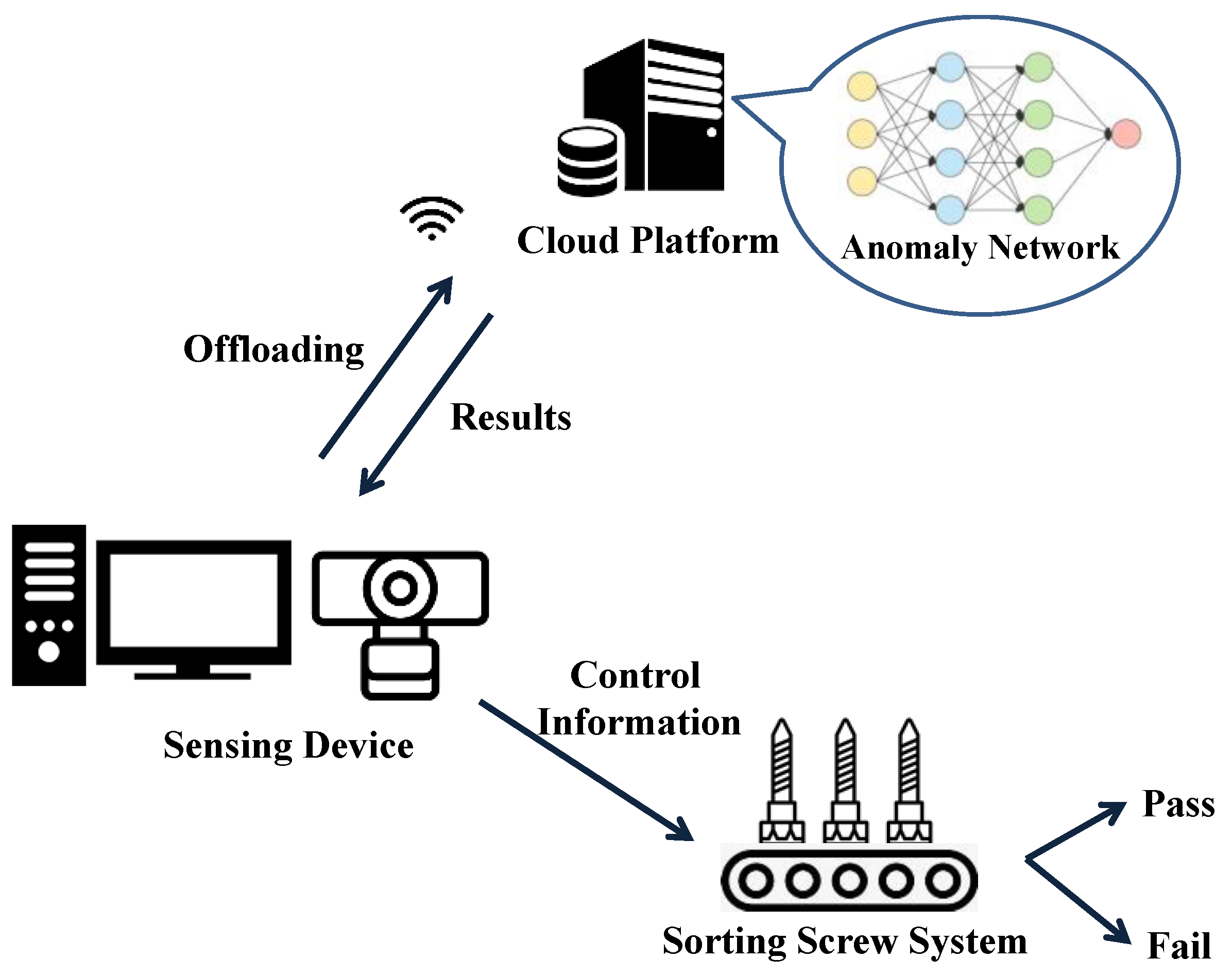
An effective method for applying deep neural networks and IoT techniques is a helpful tool to increase recognition accuracy and reduce the tiresome operation for the defective screw system operators. The proposed system mainly consists of three items, which are IIOT, sensing device, and a cloud platform. The pipeline of the framework is shown in Figure 1, in which the sensing device is coupled with a memory device and transmission interface. First, each screw product is captured by the CCD camera sensing device, and then the screw images are saved into the memory device. Moreover, the sensing device could perform the task of image preprocessing by deciding whether to offload the screw images to the cloud platform. The process of the DL model can be divided into two stages: (1) Training and (2) inference. In the case of detecting a defective screw, the screw images collected from the sensing device will be offloaded to the DL model on the cloud platform for model training through the wireless interface. Thereafter, the trained model is stored on the cloud platform. The inference process performs the prediction of the input images based on a well-trained DL model. Subsequently, the predicted results of the screw image are sent back to the sensing device, and converted into control information in order to decide whether the screw product is a Go or No Go on the production line.
2.2. Image Preprocessing of Images Stitching Technique
Template matching [21,22] is the commonly used approach for image stitching to blend the multiple images into a panoramic image, which identifies the common feature of the template image from the inspected source image. The process of template matching mainly consists of two steps. First, selecting the initial image of the spiral screw image as the template image is an important step before performing the matching process, which influences whether the defective feature is obvious after the image stitching. The next step involves finding the common characteristics of the patch for both the template and inspected images by horizontal pixel-by-pixel scanning. The maximum value of the normalized cross-correlation (NCC) is calculated to find the highest similarity of the overlapping region between the template image and inspected image. The NCC is defined as Equation (1).
where is the NCC value at coordinates ; and T are the inspected image and the template image on coordinate ; is the figure size; is the average gray value of the inspected image; and is the average gray value of the template image. The average gray value of the inspected and template images are separated and given as Equations (2) and (3).
2.3. Anomaly Detection Techniques
The defective screw feature is treated as an anomaly detection issue in this article. Two anomaly detection models, the convolutional autoencoder (CAE) and the adversarial autoencoder (AAE) are applied to detect the defective screw products. Both of these two algorithms are based on unsupervised neural network models, which do not require defective images for model training. Since it is an important part of detecting defective screw products, the details of the two anomaly detection algorithms are described below.
2.3.1. Convolutional Autoencoder (CAE)
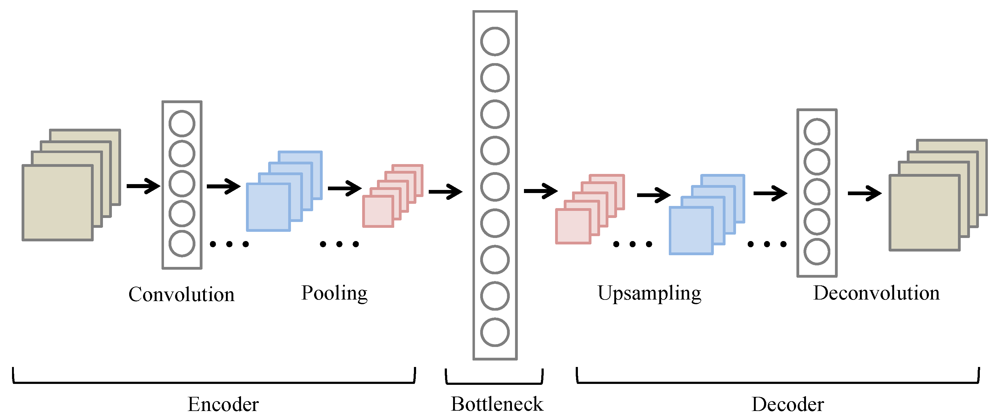
A convolutional autoencoder model has the ability to learn the hidden features from the input images without labeled ground truth. The architecture of the CAE model mainly consists of encoding and decoding. The main purpose of the encoder is not only to extract the potential features from the original input datasets, but at the same time, to reduce their dimensions. The output of the encoder is represented as a compression correlated to the input data. The decoder reconstructs the original image that is generated by the encoder. Both the encoder and decoder are trained together at the same time to attain meaningful represented features, and to be capable of restoring the original image without losing a large amount of feature information. In the CAE model, the encoder is integrated with a convolutional and pooling layer, while the decoder is coupled with deconvolutional and upsampling layers. The architecture of the CAE model is shown in Figure 2.
The definition of the encoder and decoder can be expressed as in Equations (4) and (5). The loss function of the CAE model can be obtained from the mean square error, which minimizes the error resulting from the reconstruction of the image from the original, which can be expressed as Equation (6).
where and are the encoder and decoder, respectively; and are the input image of CAE encoder and the output of CAE decoder, respectively; and is the latent feature of the CAE model. The processing of the encoder and decoder is shown in Equations (7) and (8).
where and are the activation functions of the encoder and decoder, respectively; and are the weighing of the encoder and decoder, respectively; and and are the network biases of the encoder and decoder, respectively.
2.3.2. Adversarial Autoencoder (AAE)
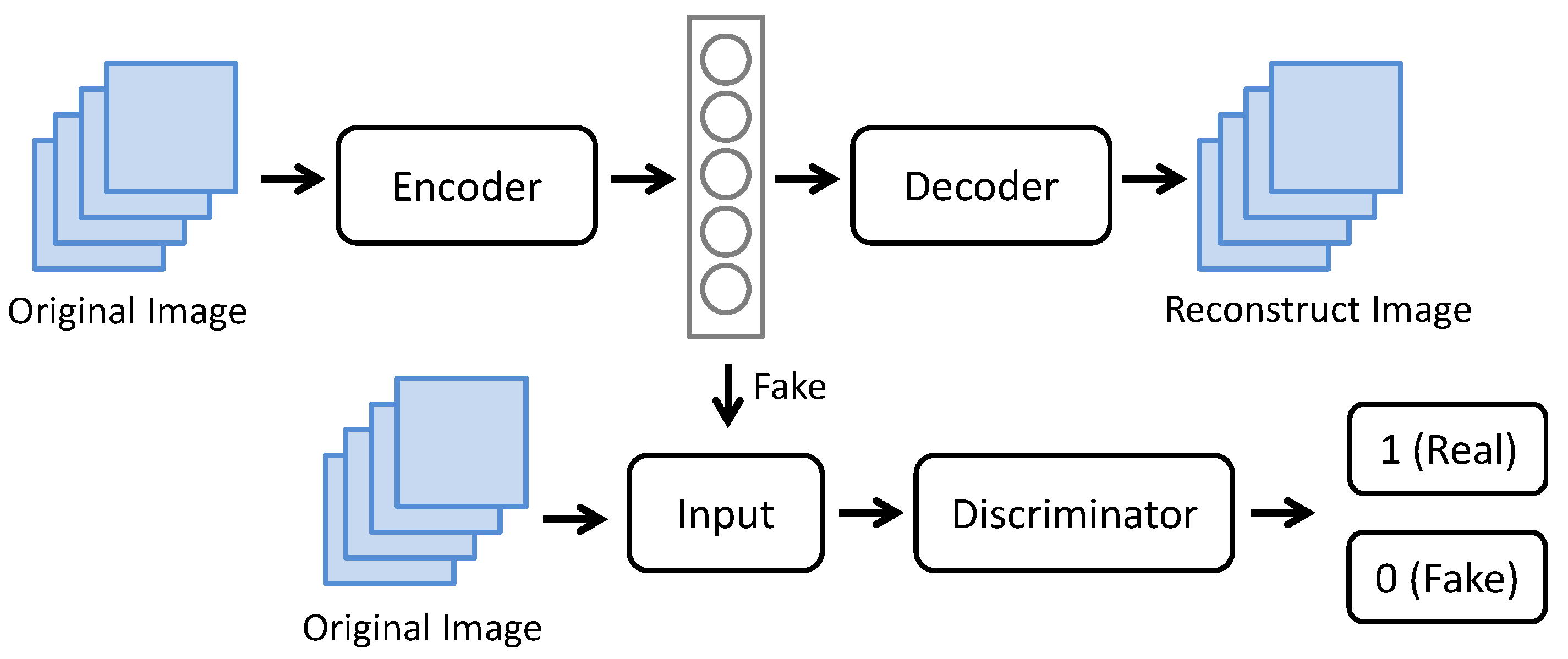
The AAE model is a kind of model variant, as introduced by Makhzani et al. [15], that combines the concept of autoencoder structure into the generative adversarial network (GAN) framework. The architecture of the AAE model is illustrated in Figure 3, which consists of two components, namely, the generator and discriminator. The autoencoder replaces the generator part of the AAE model, which contains the encoder and decoder elements to minimize the error between the reconstruction and input images. The generator is trained to fool the discriminator with the generated images. The discriminator is trained to correctly distinguish whether a latent feature of the encoder output is “normal” or a “defective” image. With an increase in training, the generated images turn out to be more realistic, whereas the discriminator could not judge the difference between the normal and defective images. Meanwhile, the discriminator is continuously trained to adapt the improved capabilities of the generator, thereby enhancing the generator and allowing it to produce more authentic normal images. The loss function of the AAE network is closed off to the AE network, which uses the Jensen-Shannon divergence (JS divergence) on an aggregated posterior distribution of latent features [23]. The loss function of the AAE network can be expressed as Equation (9).
where the parameter is denoted as the input image, and is the latent vector of the AE network. The process by which the generator converts z to x is defined as ; the encoder that converts to is defined as . is an arbitrary number appearing prior to the target distribution, and is the aggregated posterior.
3. Experiment and Discussion
To evaluate the performance of the proposed methods, template matching combined with anomaly models of CAE and AAE networks are investigated in this section. Initially, the datasets utilized in this work are described in detail. Then, three experiment parts are presented. Moreover, the template matching method is evaluated first to view the effectiveness of the merged images. Thereafter, the comprehensive results of the two anomaly networks, namely CAE and AAE, are discussed and compared to explore the detection performance. Finally, specific descriptions are provided.
3.1. Dataset Descriptions and Experiment Setup
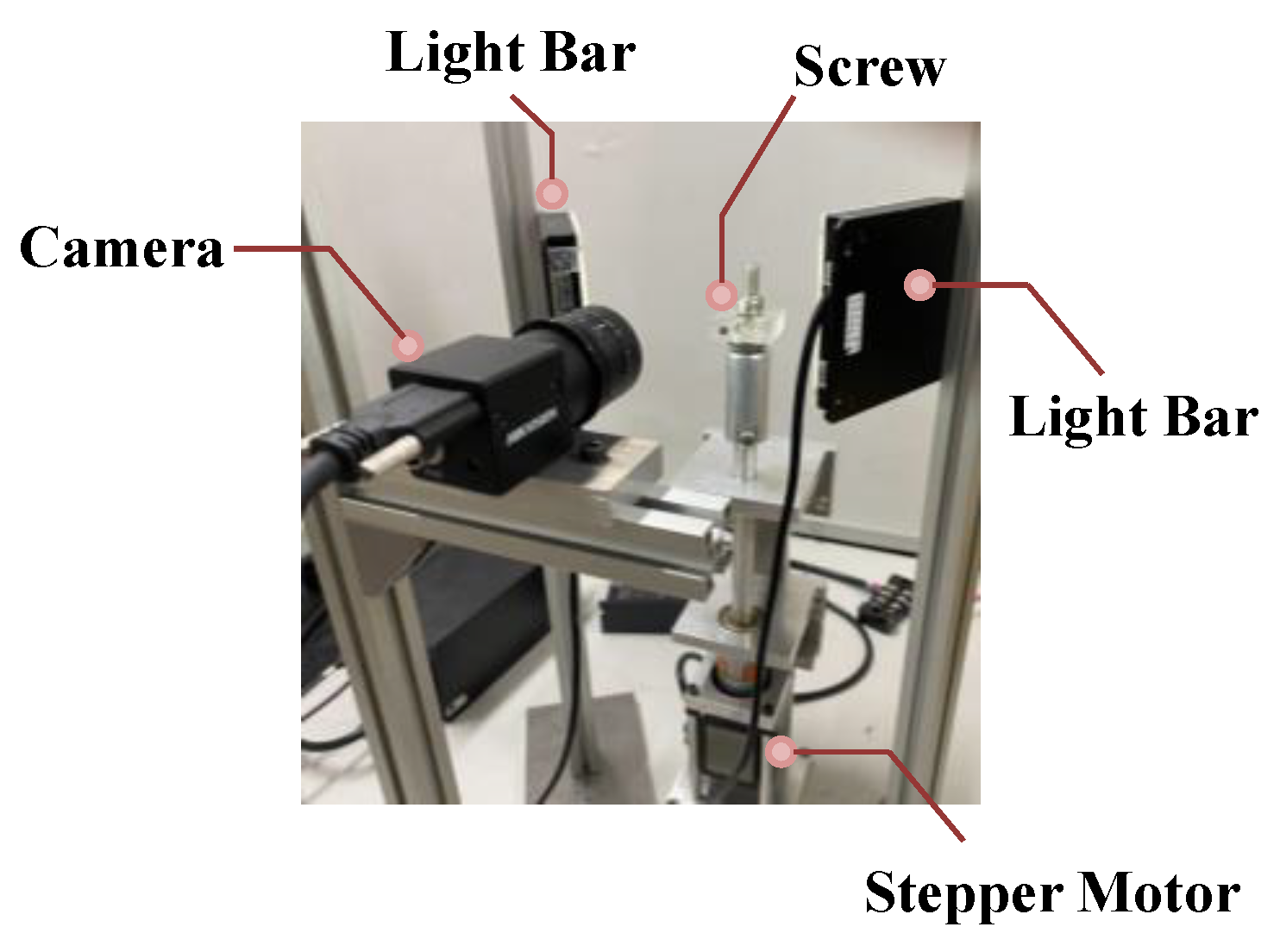
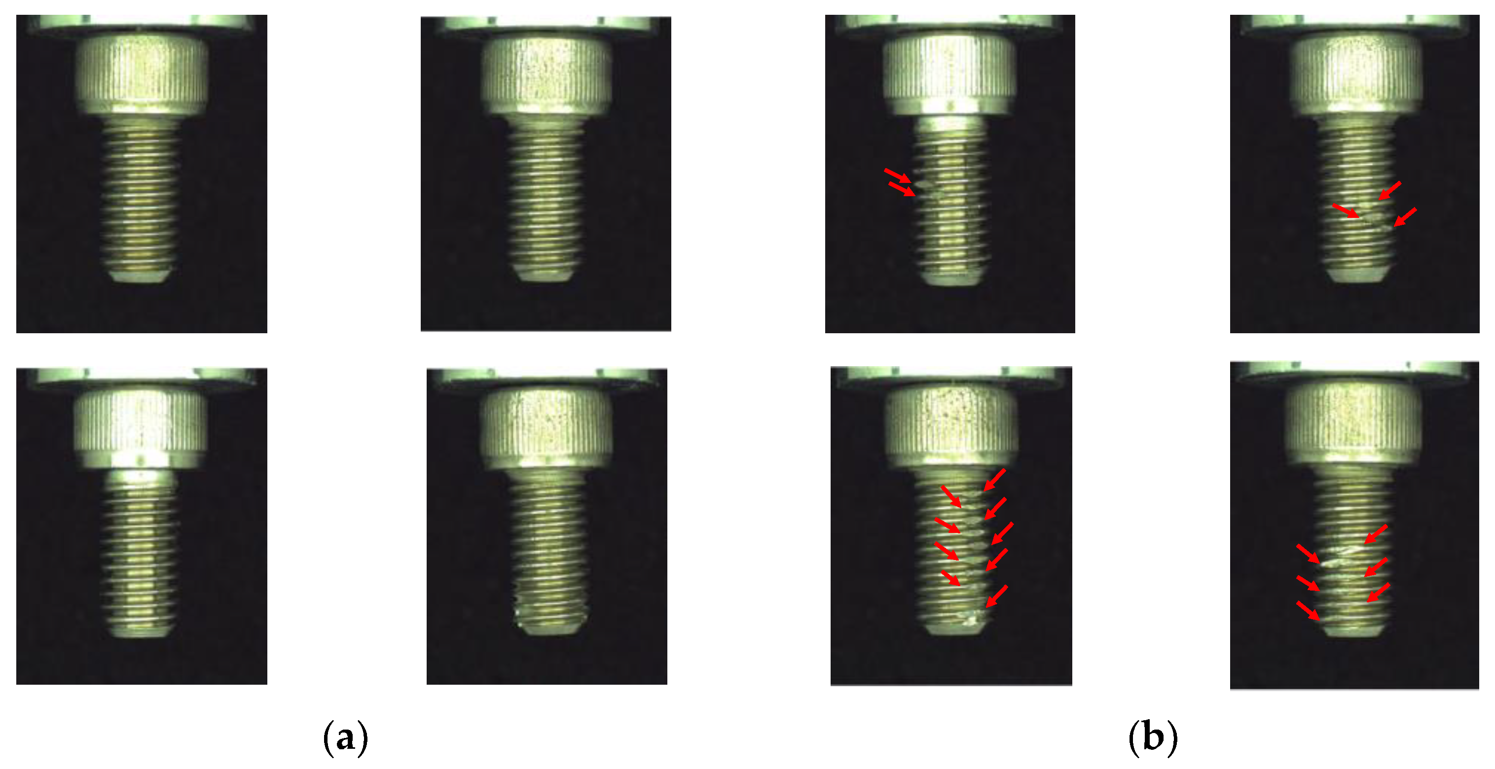
In this study, the dataset of screw images is captured from the sensing device of the developed optical instrument. The developed system of the optical instrument provides more details, as shown in Figure 4. In order to comprehensively capture the spiral screw, the developed optical instrument is designed to place the screw on the rotating plate, which is perpendicular to the lens. In addition, the stepper motor can drive the rotating plate to rotate in 360 degrees. For each screw product, about 200 images of screw images can be captured in 5 s. Moreover, the image quality is an essential factor, which will affect the result of the subsequent analysis in this study. The screw images are captured on the Hikvision camera coupled with the MORITEX lens, which can generate the high quality of the screw images. To capture the defective region on the screw more clearly, the front light of the light bars are placed on two sides of the object to create strong reflections on the screw surface. The experimental images of the spiral screw are shown in Figure 5, where the defective region on the spiral screw is indicated with the red arrow, and each image has the same scale with 762 × 920 pixels. The image resolution is approximately 0.03 mm/pixel.
Moreover, the convolutional and adversarial autoencoders are used as the core AI models for detecting the defective region on the screw image. In this experiment, both of these two networks are implemented on the cloud platform of NVIDIA GTX 1080 GPU with the TensorFlow framework. The hyper parameters of CAE were set as 8500 epochs, 0.05 learning rate, mean squared error of loss function, and Adam optimizer. The AAE model parameters were set as 10,000 epochs, 0.0002 learning rate, mean squared error and binary cross-entropy of loss function, and Adam optimizer.
3.2. Template Matching of Expanding the Spiral Screw
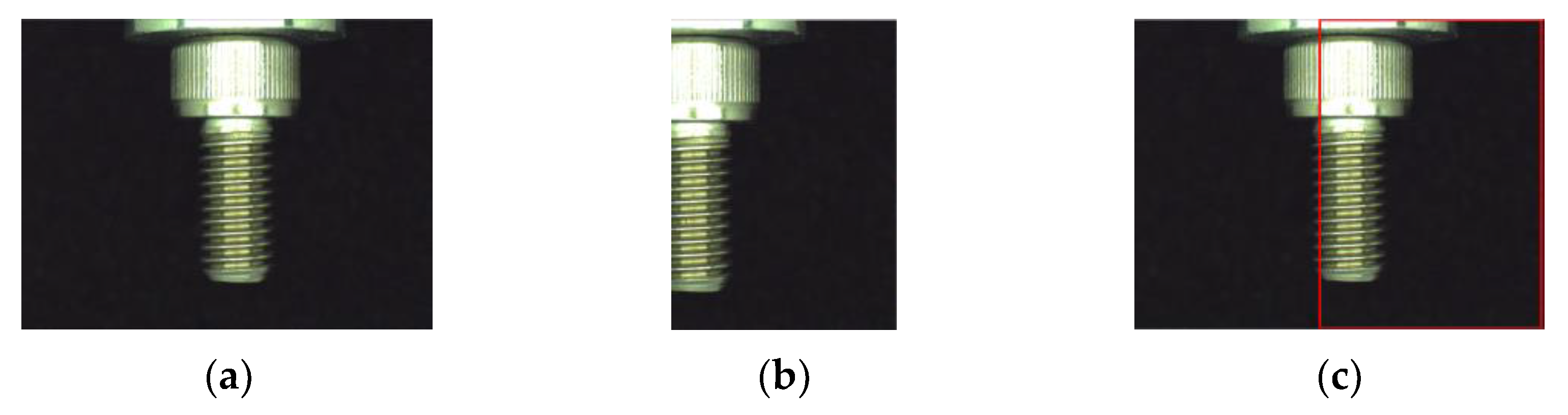
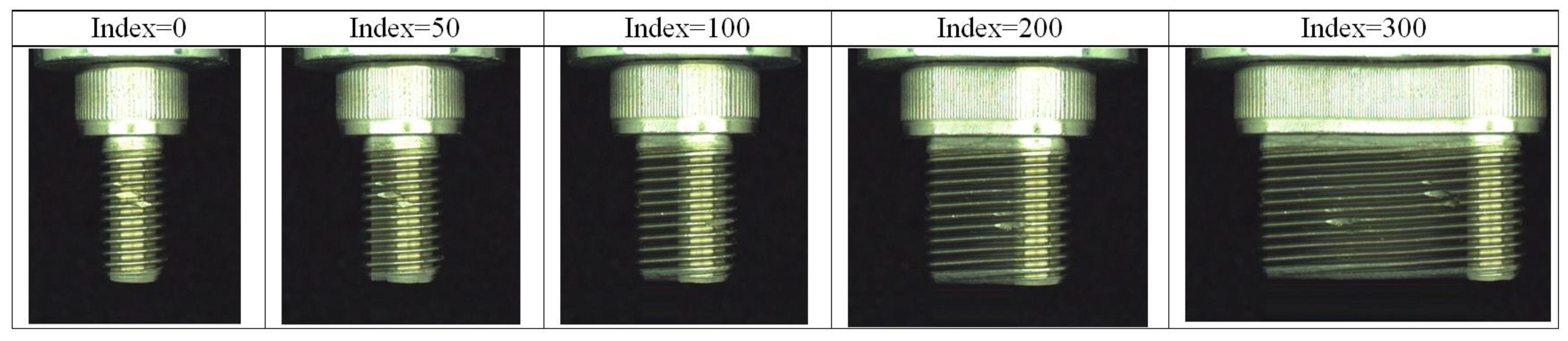
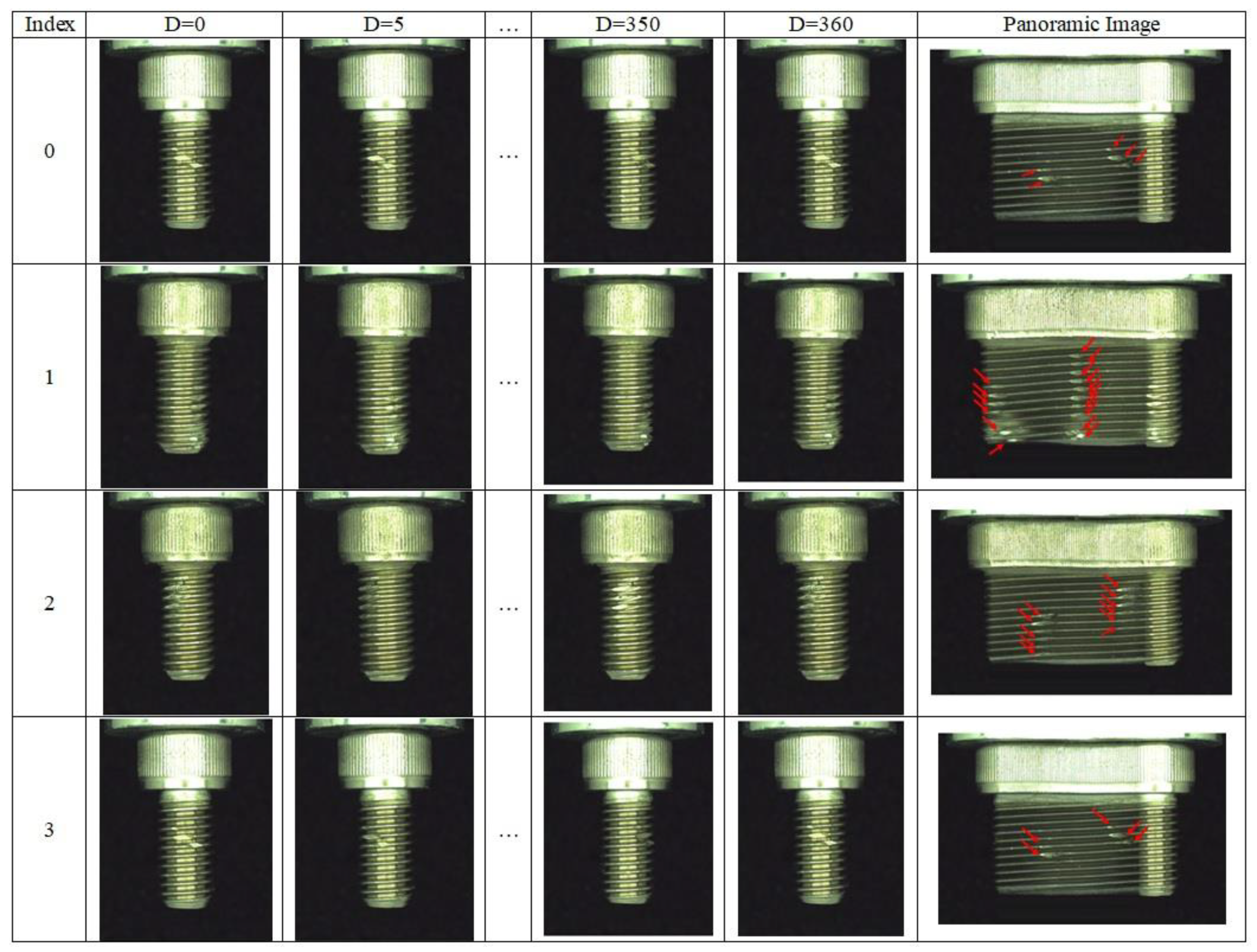
A characteristic of the screw product is the curved surface that must be turned around the screw product for detecting the defective region on the surface. The limitation of detecting the spiral screw product is selecting a specific angle to capture the defective screw region. The different capturing positions have different appearance results of the defective region. In order to address this issue, the template matching method is utilized to stitch several slices of the curved surface into a panoramic image. It is an important image preprocessing method before detecting the defective region of the screw images. The aim of the template matching approach is to find the best matched template image, which is drawn from the inspected images. The template matching process slices the template image over all the possible positions of the source image and finds the best similarity score pixel-by-pixel between the template image and the covered image. In this way, multiple slices of spiral screw images can be merged into a larger image. A schematic diagram of the template matching approach is shown in Figure 6. The template image represents the region we expected to find across the source image. The template image is compared to the source image and the highest value of correlation based on the normalized cross-correlation is calculated. The red boundary box in Figure 6c represents the region with the highest similarity to the source image. To acquire a comprehensive panoramic image, the template image will replace the overlapped region of the source image by finding the highest similarity score. The process of template matching by merging multiple sliced screw images into a panoramic image is illustrated in Figure 7. The 360 degrees of spiral screw product is captured into slice images per 1 degree in this study. In total, approximately 300 images are captured for each screw product, and seven spiral screw products are used in this study analysis. The extended panoramic image with different angles for four screw products is given in Figure 8, where the image resolution of the panoramic image is 2130 × 960 pixels. According to Figure 8, the results show that the template image can be precisely matched to the source image and successfully expanded into a panoramic image. In addition, the location of the defective screw can be clearly shown by looking at the panoramic screw image. The defective regions of the panoramic image are marked with red and indicated in Figure 8. Compared with the unstitched the screw image, the merged panoramic screw image illustrates the defective region more efficiently.
3.3. Performance of the CAE and AAE Models
3.3.1. The Patch Images Used for Study Analysis
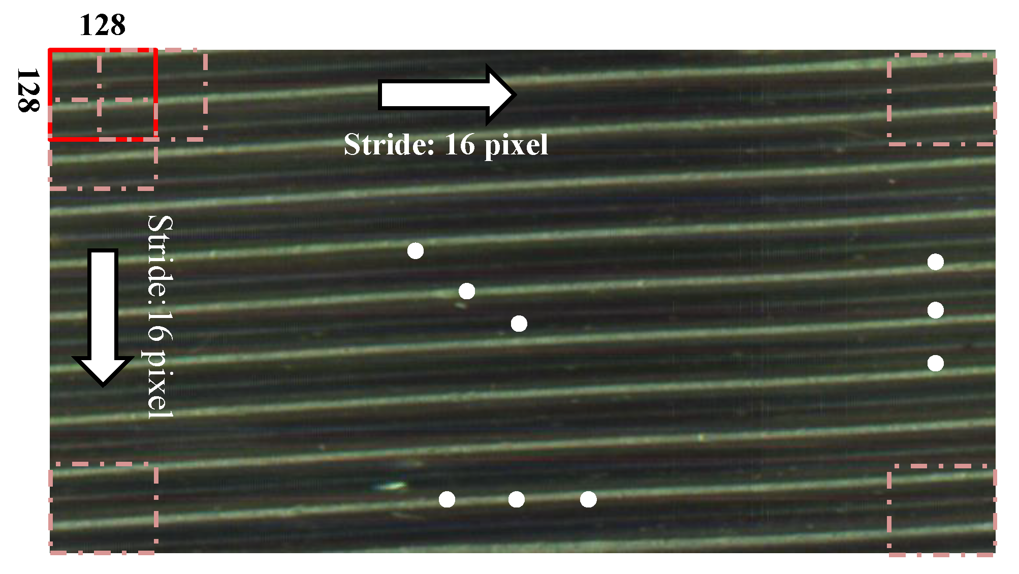
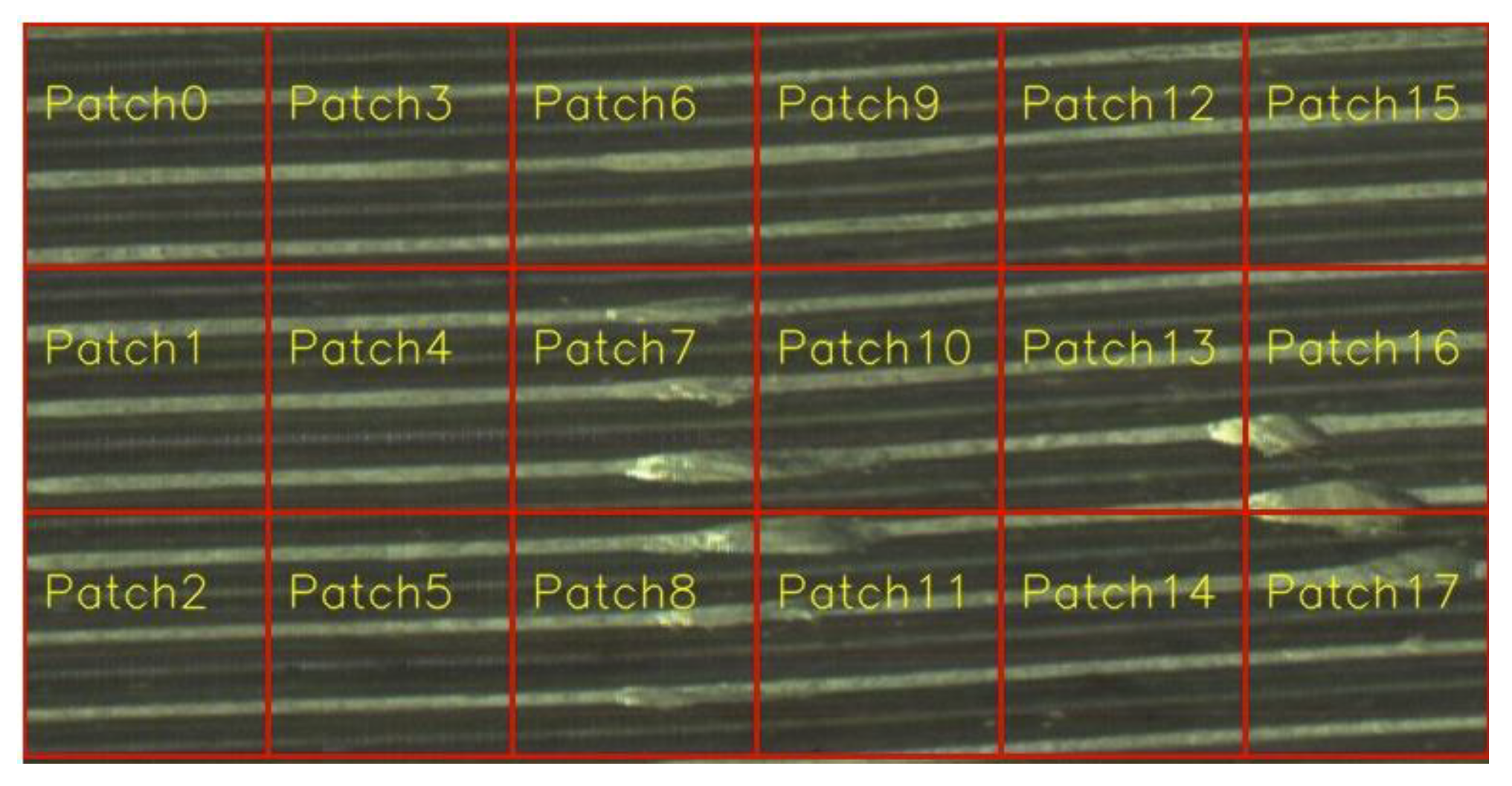
Preparing the training and testing datasets is an important process before conducting the model training and testing. The two factors will affect the training results, which are the scale of the patch image and the total number of training dataset. According to these two factors, the following description provides more details for the experiment dataset. The scale of the patch image needs to be defined at first. If the patch images are either too large or too small, this would have an effect on the model training results. For the texture of the screw image, the features in the patch image need to contain the screw stripe. If the patch images are sliced too large, the details of the features cannot be learned well. In contrast, if the patch images are sliced too small, the network cannot learn the characteristic features over the whole image. Therefore, the dimension of the patch image is selected as 128 × 128 pixels for the best scale in the experiment. On the other hand, the number of the training dataset is another factor influencing the performance of the network. In order to have better performance on the training dataset, the screw panoramic images are sliced into multiple patch images in this study, which can create a large amount of positive datasets for model training as well as learn the normal features more effectively. In our experiments, a normal panoramic screw image is selected as the training dataset. Then, the whole panoramic screw image is sliced by the sliding window method, which is depicted in Figure 9. The patch images are acquired with the sliding window of 128 × 128 pixels. In addition, 16 pixel strides move along the rows and columns. Therefore, the training dataset can be obtained by approximately 284 patch images. In the testing phase, the remaining panoramic screw images can be sliced into 25 image patches with the same scale of 128 × 128 pixels, which contains the normal and abnormal datasets. The slice patches of the panoramic screw image are shown in Figure 10, where the resolution of the panoramic screw image for the testing phase is 384 × 768 pixels. Moreover, the data augmentation method of rotation and horizontal flipping is utilized to create more datasets in this article, which can prevent overfitting during the training process. The training dataset can be increased to 10,000 patch images for network training by the data augmentation method.
3.3.2. The Meaning of Patch Image for CAE and AAE Networks
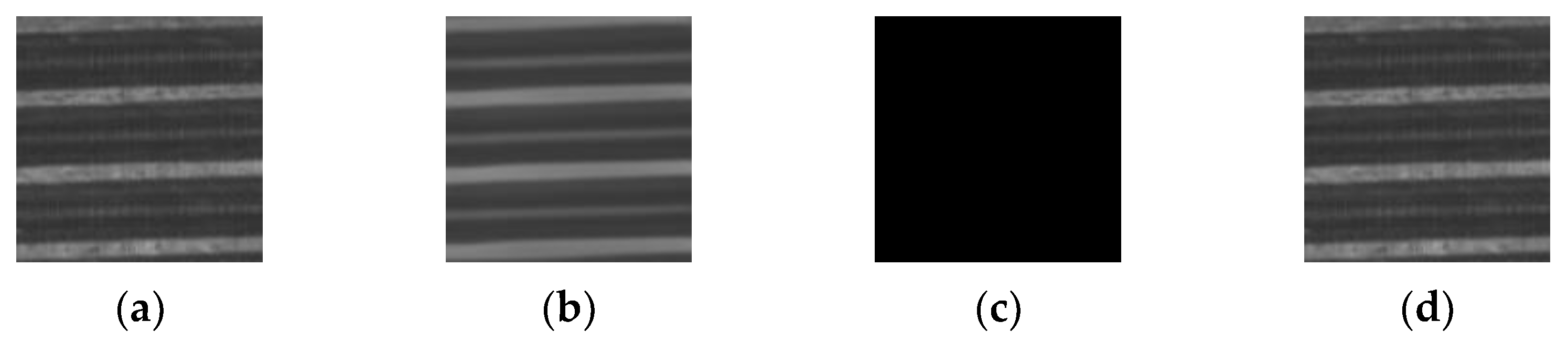
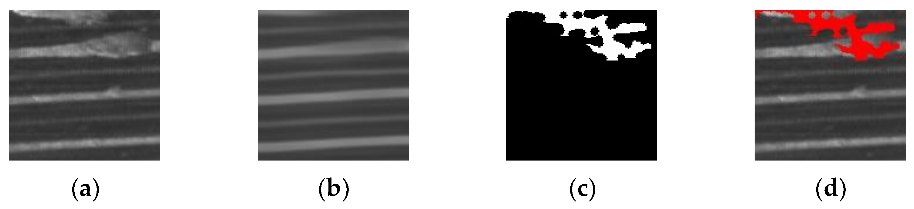
Both the CAE and AAE networks learn the normal texture of the screw dataset in the training stage. In addition, abnormal datasets are utilized during the testing stage to evaluate the model performance. Prior to comparing the results produced by the two networks, the functioning of normal and abnormal images on the network is illustrated as follows. Normal images can be utilized to examine the reconstruction ability of the network. If the reconstruction ability is great, the reconstructed image can be restored as the original image. The residual image showing the difference between the original image and the reconstructed image would not appear in the anomaly region, which would be shown as a back graph. It represents the effectiveness of the network in extracting features from the source images during the process of encoding and decoding. Furthermore, for the abnormal images, the network could restore the defective region that appears in the images to the normal reconstructed image. The residual figure can be inspected to examine the difference between the original image and reconstructed image for detecting the features of the defective texture. The meaning of the normal patch images for two networks is shown in Figure 11, where Figure 11a is the original image of normal dataset trained by the network; Figure 11b is the reconstructed image derived from the normal dataset extracted by the network; Figure 11c is the residual image taken from the normal dataset, which shows the difference between the original image and reconstructed image; and Figure 11d is a superimposed image, which combines the original and residual images taken from a normal dataset. The meaning of the abnormal patch for two networks is shown in Figure 12, where Figure 12a is the original image taken from an abnormal dataset tested by the network; Figure 12b is the reconstructed image derived from an abnormal dataset detected by the network; Figure 12c is the residual image taken from an abnormal dataset, which is the difference between the original image and reconstructed image; and Figure 12d is the superimposed image, which combines the original and residual images from the abnormal dataset. The resolution of each patch is 128 × 128 pixels in Figure 11 and Figure 12.
3.3.3. Comparison between CAE and AAE Networks
To compare the performance of the AAE and CAE networks, this study partially selects the normal and abnormal patch images of the four screw images for discussion. A comparison illustrating the detection of the screw patch images with 128 × 128 pixels taken from normal and abnormal images of the model testing are shown in Table 2. Examining the two anomaly detection networks, it can be observed that the AAE model can successfully restore the reconstructed image to the original normal image using both normal and abnormal datasets. Moreover, the AAE network has the ability to effectively recognize the defective region of the slice patch dataset.
3.3.4. Evaluation Criteria of CAE and AAE Networks
It is necessary to evaluate the predictive performance after the model training process. In this study, three evaluation criteria, the intersection over union (IoU), dice coefficient (DC), and frames per second (FPS) [24] were used to quantify the experiment results of the two anomaly networks. IoU is known to be a popular metric to calculate the overlap percentage of the common pixels between the predicted region and ground truth. The range of the IoU is from 0 to 1, where an IoU of 0 represents no overlap between the predicted region and ground truth. An IoU of 1 indicates that the predicted region and ground truth perfectly overlap. Moreover, the dice coefficient is another widely used indicator, which is similar to the IoU. The dice coefficient is used to evaluate the similarity of the predicted region and ground truth. Both of these indicators were compared with the ground truth (GT), which were provided in Equations (10) and (11).
Seven screw datasets were employed to test the two networks under the same circumstances of the model parameters, such as the epoch and learning rate. The experiment results of AAE and CAE are shown in Table 3. The quantitative detection of the two networks is given in Table 4. According to the results, the average IoU of CAE and AAE are 0.31 and 0.34, respectively and the average DC of CAE and AAE are 0.45 and 0.51, respectively. It can be found that a predictive result of the AAE is similar to the ground truth. The AAE network exhibits a higher performance than the CAE network in detecting the defective region of the screw image. Moreover, the frame per second (FPS) number is another indicator to figure out the real-time detection on the AAE and CAE networks. The different structures of the networks have different depths, which affect the recognition rate of the network. The results show that with more complexity layers of the CAE network, the detection speed is slower.
3.3.5. Synthetization of the Patch Images
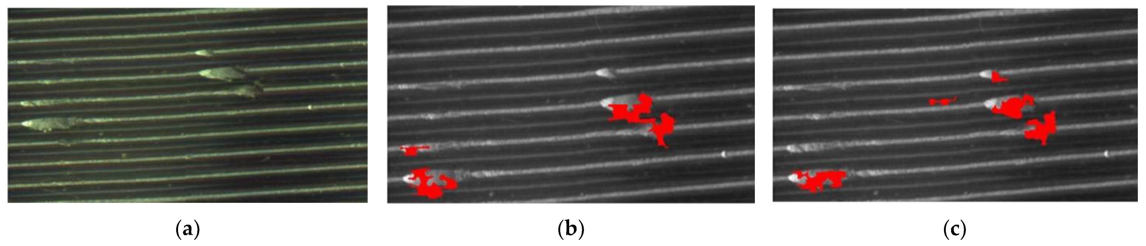
As previously stated, the CAE and AAE networks are used to train and test the slice patch images, which are generated from the original images. In order to examine the defective texture that appeared in the original screw image more clearly, this study synthesized the patch residual images to the original panoramic image. The patch images synthesized to the original panoramic image of CAE and AAE networks are shown in Figure 13. From left to right, the images include the original synthesized image, the CAE synthesized image, and the AAE synthesized image, where the CAE synthesized image is the detection result of the CAE network, and the AAE synthesized image is the detection result of the AAE network. The resolution of the synthesized image is 387 × 768 pixels in Figure 13. From an overview of these three images, it can be seen that the AAE network can comprehensively detect the defective region found in the panoramic screw image. Moreover, it indicates that the AAE network has an ability to generate a normal image more efficiently, with the result that the residual images of defective regions can be recognized with more precision.
4. Results and Discussion
The proposed smart sorting screw system integrates the image stitching technique, anomaly deep learning networks, and IoT technology to comprehensively and automatically identify the defective spiral screw products. According to the results of image stitching technique, the template matching method can merge the sliced screw image into panoramic images, which improves the effectiveness for analyzing defective images. Moreover, any rotation product problems can be detected using the template matching technique through the proposed system. The experimental results show that the AAE model can restore the abnormal region to a normal region in a better way than the CAE model. Although the quantitative results achieve a slightly lower accuracy in detecting the defective screw image, the proposed methods are more meaningful in a practical application, as it dramatically improves the traditional image processing techniques of adjusting the parameter setting. Moreover, the unsupervised learning method of learning image reconstruction overcomes the supervised learning strategy of requiring an extensive amount of normal and abnormal images for model training, which provides a breakthrough in practical industrial applications. In addition, the main challenge of anomaly detection model is the poor quality of the reconstruction image, which leads to imprecise defect localization. In future work, this study will mainly make an effort to enhance the quality of reconstruction image by adding more features or noises to the training stage, making the anomaly detection models more robust and precise.
5. Conclusions
It is important to detect the defective region that appears in a screw image during the process of quality sorting screw products. The spiral screw is characterized by a curved surface, making the process of detecting the defective region more difficult. In order to comprehensively detect the defective region of the spiral screw, a smart sorting screw system is proposed in this article. The template matching method is employed to stitch several phases of curved images into a panoramic image. Then, a panoramic screw image can be used to train and test anomaly networks more efficiently than with the other methods. The state-of-the-art unsupervised learning network of CAE and AAE models can be trained with a normal image, which can solve the issue of difficulty in obtaining the defective images taken from actual situations. Moreover, the IoT technique is utilized to upload the screw image to a cloud platform through the Wi-Fi or 4G network for training and inference. The experimental results showed that the AAE network achieves the best IoU and dice coefficient score by recognizing the defective region of the spiral screw image. Furthermore, it can reveal that the AAE network can learn the normal images well, and the characteristics of defects can be effectively identified through the residual map. The proposed smart sorting screw system based on the IoT technique can automatically detect a defective screw image as well as monitor the detection status of the entire inspection system to enhance the efficiency and performance during the detection process.
Author Contributions
W.-J.L. wrote the paper, implemented the methodology, and performed the experiments; J.-W.C. implemented the algorithms and performed the experiments; H.-T.Y. revised the manuscript; C.-L.H. designed the algorithms and revised the paper; K.-M.L. edited the manuscript and supervised the work. All authors have read and agreed to the published version of the manuscript.
Funding
This research is supported by the Ministry of Science and Technology under the grants MOST 110-2218-E-002-038.
Data Availability Statement
The data are not publicly available.
Conflicts of Interest
The authors declare no conflict of interest.
References
- Chettri, L.; Bera, R. A comprehensive survey on Internet of Things (IoT) toward 5G wireless systems. IEEE Internet Things J. 2019, 7, 16–32. [Google Scholar] [CrossRef]
- Huang, D.-C.; Lin, C.-F.; Chen, C.-Y.; Sze, J.-R. The Internet technology for defect detection system with deep learning method in smart factory. In Proceedings of the 2018 4th International Conference on Information Management (ICIM), Oxford, UK, 25–27 May 2018; pp. 98–102. [Google Scholar]
- Roman, R.; Rios, R.; Onieva, J.A.; Lopez, J. Immune system for the internet of things using edge technologies. IEEE Internet Things J. 2018, 6, 4774–4781. [Google Scholar] [CrossRef]
- Marino, R.; Wisultschew, C.; Otero, A.; Lanza-Gutierrez, J.M.; Portilla, J.; de la Torre, E. A Machine-Learning-Based Distributed System for Fault Diagnosis With Scalable Detection Quality in Industrial IoT. IEEE Internet Things J. 2021, 8, 4339–4352. [Google Scholar] [CrossRef]
- Song, C.; Xu, W.; Han, G.; Zeng, P.; Wang, Z.; Yu, S. A Cloud Edge Collaborative Intelligence Method of Insulator String Defect Detection for Power IIoT. IEEE Internet Things J. 2021, 8, 7510–7520. [Google Scholar] [CrossRef]
- Variz, L.; Piardi, L.; Rodrigues, P.J.; Leitão, P. Machine learning applied to an intelligent and adaptive robotic inspection station. In Proceedings of the 2019 IEEE 17th International Conference on Industrial Informatics (INDIN), Helsinki, Finland, 22–25 July 2019; pp. 290–295. [Google Scholar]
- Perng, D.-B.; Chen, S.-H.; Chang, Y.-S. A novel internal thread defect auto-inspection system. Int. J. Adv. Manuf. Technol. 2010, 47, 731–743. [Google Scholar] [CrossRef]
- Yang, B.; Cao, X.; Li, X.; Zhang, Q.; Qian, L. Mobile-Edge-Computing-Based hierarchical machine learning tasks distribution for IIoT. IEEE Internet Things J. 2019, 7, 2169–2180. [Google Scholar] [CrossRef]
- Chen, Y.; Lin, Z.; Zhao, X.; Wang, G.; Gu, Y. Deep learning-based classification of hyperspectral data. IEEE J. Sel. Top. Appl. Earth Obs. Remote Sens. 2014, 7, 2094–2107. [Google Scholar] [CrossRef]
- Krizhevsky, A.; Sutskever, I.; Hinton, G.E. Imagenet classification with deep convolutional neural networks. Adv. Neural Inf. Process. Syst. 2012, 25, 1097–1105. [Google Scholar] [CrossRef]
- Goodfellow, I.J.; Pouget-Abadie, J.; Mirza, M.; Xu, B.; Warde-Farley, D.; Ozair, S.; Courville, A.; Bengio, Y. Generative adversarial networks. arXiv 2014, arXiv:1406.2661. [Google Scholar] [CrossRef]
- Im Im, D.; Ahn, S.; Memisevic, R.; Bengio, Y. Denoising criterion for variational auto-encoding framework. In Proceedings of the AAAI Conference on Artificial Intelligence, San Francisco, CA, USA, 4–9 February 2017; pp. 2059–2065. [Google Scholar]
- Kingma, D.P.; Welling, M. Auto-encoding variational bayes. arXiv 2013, arXiv:1312.6114. [Google Scholar]
- Radford, A.; Metz, L.; Chintala, S. Unsupervised representation learning with deep convolutional generative adversarial networks. arXiv 2015, arXiv:1511.06434. [Google Scholar]
- Makhzani, A.; Shlens, J.; Jaitly, N.; Goodfellow, I.; Frey, B. Adversarial autoencoders. arXiv 2015, arXiv:1511.05644. [Google Scholar]
- Creswell, A.; Bharath, A.A. Denoising adversarial autoencoders. IEEE Trans. Neural Netw. Learn. Syst. 2018, 30, 968–984. [Google Scholar] [CrossRef] [PubMed] [Green Version]
- Yu, J.; Liu, J. Two-Dimensional Principal Component Analysis-Based Convolutional Autoencoder for Wafer Map Defect Detection. IEEE Trans. Ind. Electron. 2021, 68, 8789–8797. [Google Scholar] [CrossRef]
- Chow, J.K.; Su, Z.; Wu, J.; Tan, P.S.; Mao, X.; Wang, Y. Anomaly detection of defects on concrete structures with the convolutional autoencoder. Adv. Eng. Inform. 2020, 45, 101105. [Google Scholar] [CrossRef]
- Kang, G.; Gao, S.; Yu, L.; Zhang, D. Deep architecture for high-speed railway insulator surface defect detection: Denoising autoencoder with multitask learning. IEEE Trans. Instrum. Meas. 2018, 68, 2679–2690. [Google Scholar] [CrossRef]
- Mei, S.; Yang, H.; Yin, Z. An unsupervised-learning-based approach for automated defect inspection on textured surfaces. IEEE Trans. Instrum. Meas. 2018, 67, 1266–1277. [Google Scholar] [CrossRef]
- Gong, C.; Erichson, N.B.; Kelly, J.P.; Trutoiu, L.; Schowengerdt, B.T.; Brunton, S.L.; Seibel, E.J. RetinaMatch: Efficient Template Matching of Retina Images for Teleophthalmology. IEEE Trans. Med. Imaging 2019, 38, 1993–2004. [Google Scholar] [CrossRef] [PubMed] [Green Version]
- Huang, Y.; Gao, J.; Zhang, L.; Deng, H.; Chen, X. Fast template matching method in white-light scanning interferometry for 3D micro-profile measurement. Appl. Opt. 2020, 59, 1082–1091. [Google Scholar] [CrossRef] [PubMed]
- Zhou, Y.; Gu, K.; Huang, T. Unsupervised representation adversarial learning network: From reconstruction to generation. In Proceedings of the 2019 International Joint Conference on Neural Networks (IJCNN), Budapest, Hungary, 14–19 July 2019; pp. 1–8. [Google Scholar]
- Chen, J.-W.; Lin, W.-J.; Lin, C.-Y.; Hung, C.-L.; Hou, C.-P.; Cho, C.-C.; Young, H.-T.; Tang, C.-Y. Automated Classification of Blood Loss from Transurethral Resection of the Prostate Surgery Videos Using Deep Learning Technique. Appl. Sci. 2020, 10, 4908. [Google Scholar] [CrossRef]
Figure 1.
The pipeline of the proposed framework.

Figure 2.
The architecture of the CAE model.

Figure 3.
The architecture of the autoencoder model.

Figure 4.
The developed system of the optical instrument.

Figure 5.
The experimental images of the spiral screw (unit: 0.03 mm/pixel). (a) Normal image; (b) defective image.
Figure 5.
The experimental images of the spiral screw (unit: 0.03 mm/pixel). (a) Normal image; (b) defective image.

Figure 6.
The schematic diagram of the template matching approach (unit: 0.03 mm/pixel). (a) Source image; (b) template image; (c) the detective region of the template in the source image.
Figure 6.
The schematic diagram of the template matching approach (unit: 0.03 mm/pixel). (a) Source image; (b) template image; (c) the detective region of the template in the source image.

Figure 7.
The process of merging multiple slices of screw images into a panoramic image (unit: 0.03 mm/pixel).
Figure 7.
The process of merging multiple slices of screw images into a panoramic image (unit: 0.03 mm/pixel).

Figure 8.
The extended panoramic image with different angles of four screw products (unit: 0.03 mm/pixel).
Figure 8.
The extended panoramic image with different angles of four screw products (unit: 0.03 mm/pixel).

Figure 9.
The slice patches of the panoramic screw image for the training phase (unit: 0.03 mm/pixel).
Figure 9.
The slice patches of the panoramic screw image for the training phase (unit: 0.03 mm/pixel).

Figure 10.
The slice patches of the panoramic screw image for the testing phase (unit: 0.03 mm/pixel).
Figure 10.
The slice patches of the panoramic screw image for the testing phase (unit: 0.03 mm/pixel).

Figure 11.
The meaning of the normal patch for two networks (unit: 0.03 mm/pixel). (a) Original patch image; (b) reconstruct patch image; (c) residual patch image; (d) superimposed patch image.
Figure 11.
The meaning of the normal patch for two networks (unit: 0.03 mm/pixel). (a) Original patch image; (b) reconstruct patch image; (c) residual patch image; (d) superimposed patch image.

Figure 12.
The meaning of the abnormal patch for two networks (unit: 0.03 mm/pixel). (a) Original patch image; (b) reconstruct patch image; (c) residual patch image; (d) superimposed patch image.
Figure 12.
The meaning of the abnormal patch for two networks (unit: 0.03 mm/pixel). (a) Original patch image; (b) reconstruct patch image; (c) residual patch image; (d) superimposed patch image.

Figure 13.
The patch images synthesized to the original panoramic image of CAE and AAE networks (unit: 0.03 mm/pixel). (a) Original synthesized image; (b) CAE synthesized image; (c) AAE synthesized image.
Figure 13.
The patch images synthesized to the original panoramic image of CAE and AAE networks (unit: 0.03 mm/pixel). (a) Original synthesized image; (b) CAE synthesized image; (c) AAE synthesized image.


Table 1.
The comparison between supervised learning and unsupervised learning.
| Approach | Method | Strengths | Weaknesses |
|---|---|---|---|
| Supervised-based classifier | Classification network: CNN | Fast training and inference |
|
| Semantic network: U-Net, FCN | Fast training and inference; high performance of defect localization | ||
| Object detection network: YOLO, Faster R-CNN | Identify the defect with the bounding boxes | ||
| Unsupervised-based classifier | Convolutional Autoencoder; Adversarial Autoencoder | Model training without annotation; requires only positive datasets for model training |
|
Table 2.
The screw patches of dataset 1 tested for CAE and AAE networks (unit: 0.03 mm/pixel).
| Index | Original | CAE | AAE | ||||
|---|---|---|---|---|---|---|---|
| Reconstruct | Residual | Superimposed | Reconstruct | Residual | Superimposed | ||
| 1 |  |  |  |  |  |  |  |
| 2 |  |  |  |  |  |  |  |
| 3 |  |  |  |  |  |  |  |
| 4 |  |  |  |  |  |  |  |
| 5 |  |  |  |  |  |  |  |
| 6 |  |  |  |  |  |  |  |
| 7 |  |  |  |  |  |  |  |
| 8 |  |  |  |  |  |  |  |
Table 3.
The experiment results of AAE and CAE networks.
| Networks | Dice | IoU |
|---|---|---|
| CAE |  |  |
| AAE |  |  |
Table 4.
The quantitative detection of two networks.
| Model | Dice Min/Mean/Max | IoU Min/Mean/Max | FPS |
|---|---|---|---|
| CAE | 0.35/0.45/0.53 | 0.2/0.31/0.39 | 0.72 |
| AAE | 0.41/0.51/0.59 | 0.23/0.34/0.41 | 3.2 |
Publisher’s Note: MDPI stays neutral with regard to jurisdictional claims in published maps and institutional affiliations. |
© 2021 by the authors. Licensee MDPI, Basel, Switzerland. This article is an open access article distributed under the terms and conditions of the Creative Commons Attribution (CC BY) license (https://creativecommons.org/licenses/by/4.0/).
Share and Cite
MDPI and ACS Style
Lin, W.-J.; Chen, J.-W.; Young, H.-T.; Hung, C.-L.; Li, K.-M. Developing the Smart Sorting Screw System Based on Deep Learning Approaches. Appl. Sci. 2021, 11, 9751. https://0-doi-org.brum.beds.ac.uk/10.3390/app11209751
AMA Style
Lin W-J, Chen J-W, Young H-T, Hung C-L, Li K-M. Developing the Smart Sorting Screw System Based on Deep Learning Approaches. Applied Sciences. 2021; 11(20):9751. https://0-doi-org.brum.beds.ac.uk/10.3390/app11209751
Chicago/Turabian StyleLin, Wan-Ju, Jian-Wen Chen, Hong-Tsu Young, Che-Lun Hung, and Kuan-Ming Li. 2021. "Developing the Smart Sorting Screw System Based on Deep Learning Approaches" Applied Sciences 11, no. 20: 9751. https://0-doi-org.brum.beds.ac.uk/10.3390/app11209751
Note that from the first issue of 2016, this journal uses article numbers instead of page numbers. See further details here.