Using Optimisation Meta-Heuristics for the Roughness Estimation Problem in River Flow Analysis

Abstract

Climate change threats make it difficult to perform reliable and quick predictions on floods forecasting. This gives rise to the need of having advanced methods, e.g., computational intelligence tools, to improve upon the results from flooding events simulations and, in turn, design best practices for riverbed maintenance. In this context, being able to accurately estimate the roughness coefficient, also known as Manning’s n coefficient, plays an important role when computational models are employed. In this piece of research, we propose an optimal approach for the estimation of ‘n’. First, an objective function is designed for measuring the quality of ‘candidate’ Manning’s coefficients relative to specif cross-sections of a river. Second, such function is optimised to return coefficients having the highest quality as possible. Five well-known meta-heuristic algorithms are employed to achieve this goal, these being a classic Evolution Strategy, a Differential Evolution algorithm, the popular Covariance Matrix Adaptation Evolution Strategy, a classic Particle Swarm Optimisation and a Bayesian Optimisation framework. We report results on two real-world case studies based on the Italian rivers ‘Paglia’ and ‘Aniene’. A comparative analysis between the employed optimisation algorithms is performed and discussed both empirically and statistically. From the hydrodynamic point of view, the experimental results are satisfactory and produced within significantly less computational time in comparison to classic methods. This shows the suitability of the proposed approach for optimal estimation of the roughness coefficient and, in turn, for designing optimised hydrological models.

1. Introduction

To ‘ensure availability and sustainable management of water and sanitation for all’ is one of the Sustainable Development Goals (SDGs) targeted by the United Nations. Since its launch in 2015, this goal (i.e., SDG 6), assumed a wider focus and already in 2018 it was agreed that all aspects of the water cycle, being of paramount importance for development, should be considered and embedded directly and indirectly in all the remaining 17 SDGs [1].

In this context, hydraulic models are of pivotal importance to support the progress in achieving multiple SDGs. Indeed, the latter find their place in several fields of application having key implications on sustainable management of water sources [2], preserving the environment [3] and mitigating climate changes [4]. More in detail, hydraulic models can be used to predict the impact of floods, thus helping with insurance claims [5], to calculate the number of pollutants in rivers [6], estimate backwater [7] and simulate water free-surface flow [8]. Models also worth mentioning are those capable of characterising floods through sediment transport and analysis [9,10], also used to develop flood protection systems [11], and those generating flooding maps, simulating drainage channels and water temperatures [12,13,14].

Note that in the vast majority of cases, including the aforementioned studies, good models of water flows are needed to produce meaningful results. However, even if established models are nowadays available, they are sensitive to parameters that have to be found either empirically or numerically via computational methods [15]. In hydraulic engineering, such parameters typically assume two different natures:

• the ‘physical’ parameters are those describing the properties of materials—these are usually constant values;
• the empirical parameters are those added to deal with the complexity and the variability of specific aspects characterising hydraulic properties of a channel. Amongst these, the so-called ‘roughness’ coefficient, which indicates the resistance to flood flows in both channels and flood plains, is one of the most important. Other empirical parameters are the vegetation, the alignment of the channel and its irregularities, shape and size, stage and discharge, suspended sediment load and bed sediment loads. These have to be calculated mathematically through analytical models [16].

Using Mannings’s equation [17], which is expressed in terms of the roughness coefficients ‘n’, is amongst the most popular empirical methods for estimating uniform flow in open channels. In the simplest case, suggested n values can be taken from established references, where they are tabulated [18], but they can also be calculated through a number of empirical formulas [19] or field measurements. It must be remarked that the estimation of n, commonly also referred to as ‘Manning’s coefficients’, can significantly affect the final results [20]. Hence, the use of precise numerical techniques to compute such coefficients is preferred to achieve better simulations, thus allowing for more informed prevention guidelines to avoid floods and related natural disasters. Still, finding the optimal n value is a challenging task.

In 2007, Kiczko et al. [21] implemented the GSA-GLUE methodology to determine the model’s sensitivity on Manning coefficients. That analysis showed that the floodplain roughness coefficients have a small influence on flow, even though larger than that of the geometry. In the work by Romanowicz et al., in 2010 [22], a calibration model was applied to assess the Manning coefficients in solving the 1-D Saint Venant equations. In 2011 Hall et al. [23], applied a calibration methodology of a steady-state two-dimensional flood inundation model using a Bayesian approach comparing their results with previous ones based upon the same data set and flood inundation model, where the uncertainty was analyzed using GLUE. These works highlight the presence of a strong sensitivity of the empirical method for evaluating the parameters, which seems to highly depend also on the collection of suitable data. Several studies [11,24] have shown that a well-calibrated flood inundation model may perform very poorly when it is used to predict events different from those used for the calibration.

Challenges one may encounter while trying to estimate n are due to its dynamic nature. In an open channel flow context, this value is subject to variations and can significantly change over time and space. Factors responsible for such changes can be quite varied, including geometric and geomorphological factors as well as others related to the parameters characterising water currents and river beds [25], thus adding uncertainty to the estimated value.

On top of these difficulties, the average computational time for a hydrodynamic simulation using standard methodologies is of the order of hours depending on the extent of the modelled area and therefore of the computational domain.

In this light, with this piece of research, we aim to improve upon this estimation process by proposing an optimisation-based numerical approach to determine the most suitable Manning’s coefficients combination and, at the same time, to reduce, at least in a pre-processing phase, the time-consuming approach of the standard numerical solution methods. To consolidate and show the quality of our method, we apply it first to a realworld context based on the flood events of the river Paglia (an Italian river located in Umbria) occurred in 2012 and, in a second analysis, to the case of a left tributary of the Tiber river, the river Aniene.

In our study, we test several established meta-heuristics [26] for optimisation to identify the most effective ones for the specific application scenarios. Details on how to reproduce our procedures are given in the remainder of this article, which is structured as follows.

• Section 2 introduces the designed objective function which allows formulating the coefficient estimation as an optimisation problem;
• Section 3 describes the hydrodynamic computational model which is used as a blackbox component inside the designed objective function;
• Section 4 briefly recalls the five meta-heuristic considered in this work to optimise the proposed objective function;
• Section 5 presents two case studies and describes the set-up of the conducted experiments;
• Section 6 analyses the experimental results;
• Finally, conclusions are drawn in Section 7 where future lines of research are also depicted.

2. Formulating the Optimisation Problem

To obtain a framework capable of estimating optimal Manning’s coefficients, we formulate the problem as the minimisation of a ‘loss’ function whose variables are the three Manning’s coefficients for ‘left bank’, ‘central channel’ and ‘right bank’ relative to each one of the $\varsigma$ available cross-sections for the two rivers under study—see Section 5.1 and Section 5.2 for river-specific details. This results into a d-dimensional optimisation problem having $d=3·\varsigma$ real-valued design variables $x_i\in \mathbb{R}$, with $i=1,2,3,\dots ,n$, which are bounded in the range $[0.025,0.2]$. Mathematically, this means that we are looking for multivariate solutions $\mathbf{x}=[x_1,x_2,x_3,\dots ,x_d]$ within a hyper-cubical search space generated by the Cartesian product of the boundaries vectors, i.e., $\mathbf{x}\in {[0.025,0.2]}^d$.

Defining this problem analytically is not trivial, and impossible in many circumstances. However, by means of state-of-the-art simulators, it is possible to perform accurate hydrodynamic analyses in a reasonable amount of time, thus quickly estimating rivers’ depths with satisfactory accuracy. This information can then be exploited further to compute the ‘loss’ associated with the solution vectors used to run the simulation. In this study, the latter is performed by running the open-source software ‘HEC-RAS’, whose working mechanism is described in Section 3. Once the simulation is over, its output is compared with the observed depth and the absolute difference between the two values is computed to return a loss indicator.

More in detail, the objective functional call consists of the following 3 steps:

(i)

a candidate solution $\mathbf{x}$, having the previously described structure, must be produced and fed to the HEC-RAS simulator;

(ii)

HEC-RAS is set with Manning’s coefficients from the candidate solution $\mathbf{x}$ and a simulation is run to obtain the expected depth of the water at the gauge station deployed along the river—this value is referred here to as $\mathrm{HR}\left(\mathbf{x}\right)$;

(iii)

the absolute difference between $\mathrm{HR}\left(\mathbf{x}\right)$, i.e., the simulated depth, and $h_{\mathrm{obs}}$, i.e., the true depth observed at the gauge station, is calculated to obtain the loss score as shown below in Equation (1):

$$f\left(\mathbf{x}\right)=|\mathrm{HR}\left(\mathbf{x}\right)-h_{\mathrm{obs}}|.$$

(1)

It is important to note that the optimal solution for the formulated problem returns a null loss score. In other words, zero is a lower bound for Equation (1). This shows that the loss function is well-defined (i.e., negative losses cannot occur and the global minima can only return null losses).

Because of the lack of a closed-form, this problem cannot be solved theoretically. This limits the choices of suitable optimisation methods to meta-heuristic algorithms. Amongst them, we selected 5 state-of-the-art algorithms belonging to different stochastic optimisation paradigms, including evolutionary computing, swarm intelligence and Bayesian optimisation [27,28,29,30,31]. Given the black-box nature of the problem at hand, these heterogeneous set of algorithms has been purposely chosen to compensate for the absence of information on the so-called ‘fitness landscape’ of the objective functions—also referred to as fitness function in the field—which prevents us from knowing a-priori which heuristic will perform best.

3. Hydrodynamic River Flows Analysis

To carry out the hydrodynamic analysis, we made use of an established software platform developed by the U.S. Army Corps of Engineers known as HEC-RAS [32].

HEC-RAS has multiple functionalities and allows e.g., for calculating water surface profiles; energy grade lines in 1D and/or 2D and working out both steady and unsteady states; performing the so-called ‘gradually varied’ flow analysis [33]. In this study, this platform was employed for carrying out the one-dimensional steady hydraulic calculation of the rivers under investigation.

To understand how this is done, we provide further theoretical and technical details on the employed hydrodynamic model in the following section.

3.1. Mathematical Formulation and Software Settings for Implementing the Model

The simulations run for this piece of research are based on the ‘steady 1D case’ computational model, which is mathematically described with the energy equation below

$$z_1+h_1+{\alpha }_1\frac{v_1^2}{2g}=z_2+h_2+{\alpha }_2\frac{v_2^2}{2g}+h_e,$$

(2)

where

• z indicates the bottom elevation of the river;
• h is the river’s water depth;
• v is the water’s mean velocity in the channel cross-section at hand;
• the so-called St. Venant coefficient $\alpha$ is a correction factor that takes into consideration undesired effects due to e.g., non-uniformity of the water’s velocity in the considered profile of the river;
• g is the universal gravitational constant.

It is worth pointing out that Equation (2) represents the case of gradually-varying flows with suitable hydrostatic pressure distribution.

This model is implemented in the latest version of HEC-RAS, i.e., version 5.0.7 (as at the time of writing this article), which allows for setting the geometric data of the river in the convenient form of ‘geo-referenced’ files. Typically, these files follow the DEM (Digital Elevation Model) file format, as graphically shown in Figure 1. Setting the geometry for the simulation is an important step, which has to be concluded with implementing adequate upstream and downstream boundary conditions. The coordinate of the cross-sections of the river must be too defined by entering both the river station and elevation points from the left to the right bank in sequence along the river. A different number $\varsigma$ of cross-sections are allocated along the the two rivers in this research:

• $\varsigma =20$ is used for the Paglia river—located as displayed in Figure 1a;
• $\varsigma =40$ is used for the Aniene river—located as displayed Figure 1b;

From this setting, it can be immediately noticed that estimating the Manning’s coefficients for the Paglia and Aniene rivers with the method described in Section 2 results in optimising Equation (1) at $n=60$ and $n=120$ dimension values, respectively.

After having defined the geometry, the river’s discharge data need to be made available with the platform-specific file format to finalise the 1D steady model in HEC-RAS.

At this point, the model can be used. Internally, HEC-RAS uses an empirical Manning’s equation to simulate the relation between the river discharge, hydraulic resistance, river geometry, and friction energy loss. This has the form reported in Equation (3)

$$Q=K·S_f^{1/2},$$

(3)

where Q is the flow rate, or discharge, and K is the conveyance of the channel.

HEC-RAS also deals with possible changes in the channel’s geometry by assessing energy losses by using ‘contraction’ or ‘expansion’ coefficients. These are multiplicative factors for the change in the ‘velocity head’ [32]. To compute the ‘head loss’ between two sections, Equation (4) is used, while the water surface is calculated through the energy equation reported in Equation (5) [32].

The analytical expression of the energy head loss $h_e$ is as follows

$$h_e=L·S_f+C\left(\frac{{\alpha }_1{v}_1^2}{2g}+\frac{{\alpha }_2{v}_2^2}{2g}\right),$$

(4)

where $S_f$ is the energy slope, g is the gravitational acceleration, C is the expansion/contraction coefficient, L is defined in Equation (6); ${\alpha }_1$ and ${\alpha }_2$ are the velocity weighting coefficients, while $v_1$ and $v_2$ the average velocities.

The water surface level h is formally described by

$$h=Z+y+\frac{\alpha v^2}{2g}.$$

(5)

where Z is the river’s bed elevation, y is the depth of flow, $\alpha$ is the kinetic energy correlation coefficient, and v is the average velocity.

Note that, in these equations, the subscripts 1 and 2 denote two different cross-sections in the same channel reach. The basic assumption is that the cross-section number 1 is located upstream of the cross-section number 2.

To complete the description, the equation defining the distance weighted reach length L is made available below:

$$L=\frac{L_{lob}{\overline{Q}}_{lob}+L_{ch}{\overline{Q}}_{ch}+L_{rob}{\overline{Q}}_{rob}}{{\overline{Q}}_{lob}+{\overline{Q}}_{ch}+{\overline{Q}}_{rob}},$$

(6)

where the subscripts $lob$, $ch$, $rob$ referred to the left overbank, main channel, and right overbank respectively. The quantity $({\overline{Q}}_{lob}+{\overline{Q}}_{ch}+{\overline{Q}}_{rob})$ represents the arithmetic average of the flows between the sections of the left overbank, the main channel and the right overbank.

It should be stressed out that the $h_e$ term plays a fundamental role, as it includes the effects of the channel contraction and extension and the related friction losses caused by both the riverbed and banks on the flowing water. If the depth is known in one crosssection, it may be also determined in the second cross-section. This value must be available to calculate the depth distribution along the channel, with the cross-sections being the inlet or the outlet boundary of the channel reach. For this reason, in hydraulic jargon, this is also referred to as the ‘boundary condition’. It has also to be noted that the kinematic energy terms and the friction losses depend on the magnitude of the flow quantified with the discharge term Q. Moreover, this model takes also into consideration the influence of floodplains while calculating St. Venant coefficients and the weighted distance between cross-sections.

The approached used in HEC-RAS to determine both the total conveyance and the velocity coefficient for a specific cross-section, requires separating the water flow into sections where velocities can be considered uniformly distributed. This is obtained by dividing the river’s flow in the overbank areas by using the cross-section break-point values (locations where n-values change). Then, the conveyance is calculated within each subdivision through Equation (3).

The empirical correlation between Manning’s equation and Manning’s coefficient is then given by the conveyance coefficient K of each ordained subdivision. This is expressed as follows

$$K=\frac{1.486}{n}A{R}^{2/3},$$

(7)

where n is the Manning’s roughness coefficient, A is the flow area and R is the hydraulic radius (area/wetted perimeter)—all terms refer to a specific subdivision and can significant vary in different subdivisions.

The HEC-RAS software program sums up all the incremental conveyances in the overbanks to obtain a conveyance for the left overbank and the right overbank. Note that the conveyance o the main channel is commonly computed as a single conveyance component. Then, the three subdivision conveyances (i.e., ‘left’, ‘channel’ and ‘right’) are summed up to obtain the total conveyance for the cross-section.

A single Manning’s n can be used for multiple sections or calculated for each section (i.e., ‘left’, ‘channel’, ‘right’).This study uses a number of $3\varsigma$ Manning’s roughness coefficients, as indicated in Section 3.1.

On top of evaluating these Manning’s n-values by solving the optimisation problem formulated in Section 2, for the sake of completeness and comparison, we also adopt the standard approach. This consists in considering tabulated values by Chow [18], which are displayed in Figure 2.

4. The Employed Optimisation Methods

Five meta-heuristics have been selected to form a varied pool of algorithms to optimise the fitness function of Section 2. A detailed description of these optimisers is given in the following sections.

4.1. (1 + 1)-ES

Evolution Strategies (ESs) [34] were first designed in the 70s and still play a key role in evolutionary computing. They evolve a set of $\mu$ solutions, called parent solutions, to generate $\lambda$ child solutions. At the end of every algorithmic cycle, a new population is made by selecting solutions amongst the available ones. This can occur according to two mechanisms. One is the so-called ‘comma’ method, indicated with the notation ‘($\mu$,$\lambda$)’, where the best child solutions are selected without considering the parent population. Alternatively, the so-called ‘plus’ strategy can be used. The latter, indicated with the notation ‘($\mu$ + $\lambda$)’, consists in creating the set containing the solution from both parent and child populations, sorting them according to their fitness values (i.e., the lower the better for a minimisation problem), and finally taking the subset of the first $\mu$ fittest solutions to create a new population.

In this work, we employs the simple configuration ($\mu$ + $\lambda$)-ES with $\mu =\lambda =1$, thus resulting to the (1 + 1)-ES algorithm. This is a trajectory-based algorithm that iteratively evolves a single solution $\mathbf{x}\in {\mathbb{R}}^d$. During each generation, a child solution $\mathbf{y}\in {\mathbb{R}}^d$ is generated using a Gaussian perturbation as shown below

$$y_j=x_j+N\left(0,{\sigma }_j^2\right),\mathrm{for}j=1,\dots ,d$$

to be subsequently compared with its parent solution x. If $\mathbf{y}$ is fitter than $\mathbf{x}$, $\mathbf{y}$ replaces $\mathbf{x}$ in the next population (x is kept otherwise).

In our experiments, the initial point $x_0$ is set to the centre of the search space, i.e., $x_{0,j}=L_j+(U_j-L_j)/2$, for $j=1,\dots ,d$, where $L_j$ and $U_j$ are the lower and the upper bound for the jth dimension respectively. The Gaussian’s variance is set as ${\sigma }_j=(U_j-L_j)/5$, with $j=1\dots ,d$.

4.2. Differential Evolution

The Differential Evolution (DE), originally proposed in [35], is a peculiar metaheuristic with a simple algorithmic structure, similar to the one of swarm intelligence algorithms, and unusual use of variation operators from the evolutionary algorithms field [36]. Indeed, in DE, N individuals ${\mathbf{x}}_1,\dots ,{\mathbf{x}}_N\in {\mathbb{R}}^d$ are evolved by means of a ‘differential mutation’ operator, which generate the ‘mutant’ solution. The latter is then crossed over with the currently processed individual to generate offspring. This newly generated solution competes with its parent and the winner will enter the new population only at the end of a whole generation cycle (i.e., after having produced N offspring solutions).

Several mutation operators are available in the literature, and two main crossover operators are usually employed. The combination of such operators give rise to several DE variants. By using common DE jargon [36,37], the DE algorithm employed in this study is fully described with the notation DE/current-to-best/1/bin. This means that the mutation operator will produce a mutant vector ${\mathbf{v}}_i$ from the generic ith solution ${\mathbf{x}}_i$ ($i=1,\dots ,N$) by following the popular current-to-best scheme reported below

$${\mathbf{v}}_i=x_i+F·({\mathbf{x}}_{\mathrm{best}}-{\mathbf{x}}_i)+F·({\mathbf{x}}_{r_1}-{\mathbf{x}}_{r_2}),$$

where ${\mathbf{x}}_{\mathrm{best}}$ is the best individual in the current population $F\in (0,2]$ is the scale factor, ${\mathbf{x}}_{r_1}$ and ${\mathbf{x}}_{r_2}$ are two distinct and randomly chosen individuals from the population (${\mathbf{x}}_i$ excluded).

Subsequently, the crossover operator will generate a target vector ${\mathbf{y}}_i$ by recombining ${\mathbf{x}}_i$ and ${\mathbf{v}}_i$ according to the binomial crossover described below:

$$y_{i,j}=\left\{\begin{array}{cc}{\mathbf{v}}_{i,j}\hfill & \mathrm{if}{r}_j<CR \mathrm{or} j=\overline{j}\hfill \\ {\mathbf{x}}_{i,j}\hfill & \mathrm{otherwise},\hfill \end{array}\right.$$

where j indicates the jth component of a solution (i.e., $j=1,\dots ,d$), $CR\in [0,1]$ is the crossover rate, $r_j$ is a randomly distributed number in $[0,1]$ and $\overline{j}$ is a random integer index in $\{1,\dots ,d\}$ ensuring that at least one component is inherited from the mutant vector. Further details on this optimisation paradigm are available at [36,38,39,40,41,42,43].

Due to the computational complexity of the problem addressed in this study, it is not possible to set a high computational budget for the optimisation process. Hence, we initialise the population of our DE algorithm by using the Scrambled Hammersley procedure [44]. This produces a low discrepancy sample of vectors, thus allowing for a better covering of the search domain since the beginning of the optimisation process. To run the algorithms, we set $N=30$, $F=0.8$ and we randomly draw a $CR$ value in $[0,1]$ any time the crossover operator is called.

4.3. Covariance Matrix Adaptation Evolution Strategy

The Covariance Matrix Adaptation Evolution Strategy (CMA-ES) [45] represents one of the most sophisticated forms of ES algorithms. It evolves the mean value and the covariance matrix of a multivariate Gaussian distribution used to draw new solutions in the search space. At each iteration, new individuals are drawn and their fitness values are evaluated. The fittest individuals are involved in the update procedure so that new distribution is moved, re-shaped and rotated to better guide the search towards promising basins of attraction. While converging, the Gaussian distribution is expected to become a good local approximation of the Hessian matrix of such basin, thus driving the population towards the local optimum.

Mathematically, the mean vector is obtained via a weighted average of the fittest individuals, which implements a multi-parent arithmetic crossover operator, while a more computational expensive procedure is required to update the covariance matrix [45,46,47].

For the sake of brevity, we point to [45,48] for technical details, and to [49] for implementation details and parameter setting other than the population size $\lambda$, which we set to 30.

4.4. Particle Swarm Optimisation

The Particle Swarm Optimisation (PSO) algorithm, initially proposed [50], is the most established swarm intelligence working logic for optimisation purposes. It iteratively updates a swarm of N particles $x_i\in {\mathbb{R}}^d$, with $i=1,2,3,\dots ,N$, each one being associate with its ith velocity vector ${\mathbf{v}}_i\in {\mathbb{R}}^d$ and personal best position $p_i\in {\mathbb{R}}^d$.

The best solution amongst the best local position ever visited by each particle is constantly updated at each iteration to keep track of the global best (so far) solution $\mathbf{g}\in {\mathbb{R}}^d$ ever visited by the entire swarm. This is the solution returned when the optimisation process is stopped.

During each iteration, velocity vectors are updated and used to perturb the position of each ith particle as follows:

$$v_{i,j}=w{v}_{i,j}+c_1{r}_{1,j}(p_{i,j}-x_{i,j})+c_2{r}_{2,j}(g_j-x_{i,j})\mathrm{for}j=1,\dots ,d,$$

$$x_i=x_i+v_i,$$

where $w,c_1,c_2>0$ are the inertial, cognitive and social coefficients respectively, while $r_{1,j}$ and $r_{2,j}$ are two randomly generated numbers in $[0,1]$.

In our experimentation we used $N=30$ and set $w=0.72$ and $c_1=c_2=1.19$ as indicated in [49]. More information on the role played by the parameters within the PSO search are available at [38,51].

4.5. Bayesian Optimisation

The Bayesian Optimisation (BO) algorithm [30] is a surrogate-based method often applied to deal with computationally expensive optimisation problems.

It consists in building a probabilistic model, i.e., the surrogate model, to approximate the fitness function and make fast predictions on its values for any solution $\mathbf{x}\in {\mathbb{R}}^d$ generated through the acquisition function. The true fitness function f must be also used to obtain the $f\left(\mathbf{x}\right)$ value required to update the surrogate model, thus decreasing the level of uncertainty when looking within a neighbourhood of the point $\mathbf{x}$. As for most heuristics, the process is stopped when a maximum number of fitness functional calls is reached. Details on this algorithm are available at [30].

In our experimental phase, we adopt the Gaussian Processes and the Upper Confidence Bound as surrogate model and acquisition function respectively. Note that these are the most common configuration and normally lead to satisfactory performances [30]. Moreover, for the sake of consistency, we set the populating size of the BO algorithm equal to $N=30$, and sample the initial population of candidate solutions with the Scrambled Hammersley procedure, see [44], in order to have a ‘diverse enough’ initial surrogate model.

5. Experimental Set-up

We apply the five meta-heuristics described in Section 4 on the objective function formulated in Section 2 and we compare their performances as reported at the end of Section 3.1.

The Python’s platform Nevergrad 0.4.2 is used to run the five selected algorithms, whose code is available at [49,52], on a machine running Windows 10 and equipped with an Intel Xeon E5-2650v4 processor clocking at 2.20 GHz, with 128 GB of RAM. Note that this experimentation phase can be replicated on different machines as long as a COM interface is available, for handling the inter-process communications between the Python’s platform and the HEC-RAS simulator [53], and an MS Windows operating system is used. This is due to the necessity of running HEC-RAS, which forms the core of our objective function and it is only available for these operating systems.

We address two case studies based on the Paglia and Aniene rivers, for which we used a number of cross-sections $\varsigma =20$ and $\varsigma =40$ respectively for executing the simulator. As previously mentioned in Section 2, this results in two different search spaces as the number of design variables to be optimised depends on the availability of cross-sections according to the formula $d=3\varsigma$, which means that we are solving a 60-dimensional problem for the first river and a 120-dimensional one for the second river. Further details on the two rivers are provided in Section 5.1 and Section 5.2 repressively.

For both the case studies, and regardless of the optimisation algorithm, we fixed a maximum execution time 0f 600 s for performing the optimisation process. This means that, on average, each algorithm performs the optimisation on 300 fitness functional evaluations for the Paglia river and 220 fitness functional evaluations for the Aniene river. To provide statistical evidence on the performances of the algorithms considered in this study, we execute them 25 times on both case studies.

The employed parameter settings for the algorithms is reported in Section 4, and all of them have been equipped with the Nevergrad built-in ‘clipping’ constraints handling method to deal with out-of-bounds violations of the search space as described in Section 2.

5.1. Case Study 1—The River Paglia

The first case study is based on the analysis of data selected from the hydrographic service of the Umbria Region, available online at https://www.regione.umbria.it/ambiente/servizio-idrografico, accessed on 11 November 2020, related to a single reach of the Paglia river during the flood event occurred in 2012.

It is worth reporting that the river Paglia originates from an extinct volcano, i.e., the Amiata mountain, at 1738 meters above sea level. It flows from upstream to downstream towards the plain of the city of Orvieto and its course, which crosses the three Italian regions Toscana, Umbria and Lazio, the riverbed is mainly made up of gravelled and rocky materials with short grassy banks depending on the seasons. The hydrographic framework of this river has a basin of 1187 km² and an average flow rate of 11.3 m³/s. Its entire basin is generally characterised by low permeability materials, about $75\%$, and its slope is averaged at $4.8‰$ up to its confluence with the canal Subbisone. This first stretch is followed by a steeper one, of 7‰ between this confluence and the Mount Rubiaglio, and by a final stretch sloping at about $3.3‰$ (which is the one under investigation for this study).

To evaluate the proposed optimisation procedure, we collected relevant data referring to a specific event taking place in the selected area of study Figure 3.

During the night between the 11th and 12th of November 2012, pluviometers registered a massive rainfall leading to a peak discharge of 307 mm at the gauging station of the Orvieto Scalo area. This area corresponds to the cross-section labelled with ‘12,850’, as shown in Figure 4.

This event is of particular interest for our analysis as it produced a considerable rise in the hydrometric levels, thus generating deleterious overflows resulting in major damages in many villages and cities in the surrounding area. Note that the registered peak discharge, which we use as the upstream boundary condition for our study, was equal to $Q=2200$ m³/s.

All the performed simulations for this case study are based on the 1D steady condition for its fast computational time.

5.2. Case Study 2—The River Aniene

The second case study presents a stronger focus on risk mitigation practises and their implementation through the proposed computational approach, thus posing the attention on a different hydrodynamic aspect.

More specifically, in the objective function the observed water surface elevation value $h_{\mathrm{obs}}$ is the outcome of a previous simulation performed with the standard approach where the Manning’s n values are taken from the empirical tables). Such value is then compared to the ‘expected’ target limit value $\mathrm{HR}\left(\mathbf{x}\right)$ imposed by the geomorphological shape of the riverbed. The latter is calculated to prevent flooding.

This time, we consider the reach of the Aniene river forming a significant portion of the catchment of the river Tiber. This is an important stream crossing six different Italian regions and, even if only marginally, Vatican City. Its length is 99 km and it drains a catchment of 1414 km².

We focus our analysis on the section of this river surrounding the town of Tivoli, as shown in Figure 5. This area features an ancient roman bridge crossing the course of the river thus forming, from a hydrological standpoint, a discontinuity in the computational field. This makes this case study more interesting but also more challenging due to the need of a more complex computational model.

Note that the riverbed characteristics are more homogeneous with respect to those of the previous case study, with short, high permeable grassy plains depending of course on the seasons. The different feature here is represented by the presence of a few man-made constructions right near the river banks: this occurrence, together with a deeper shaped riverbed, generally guarantees a more controlled water flow and decreases the risk of flooding in the entire basin.

Not having an actual real data station, the cross-section selected to be evaluated in the objective function in this case is the first one, labelled with “2” (see Figure 1b)and the overall discharge considered is $Q=400$ m³/s. Evidence of the simulation results are reported in Figure 6.

It has to be noted how in this second analysis, where the geometry, hence the computational area, is smoother, we were able to perform a steady hybrid 1D-2D simulation, thus improving the quality of the obtained results.

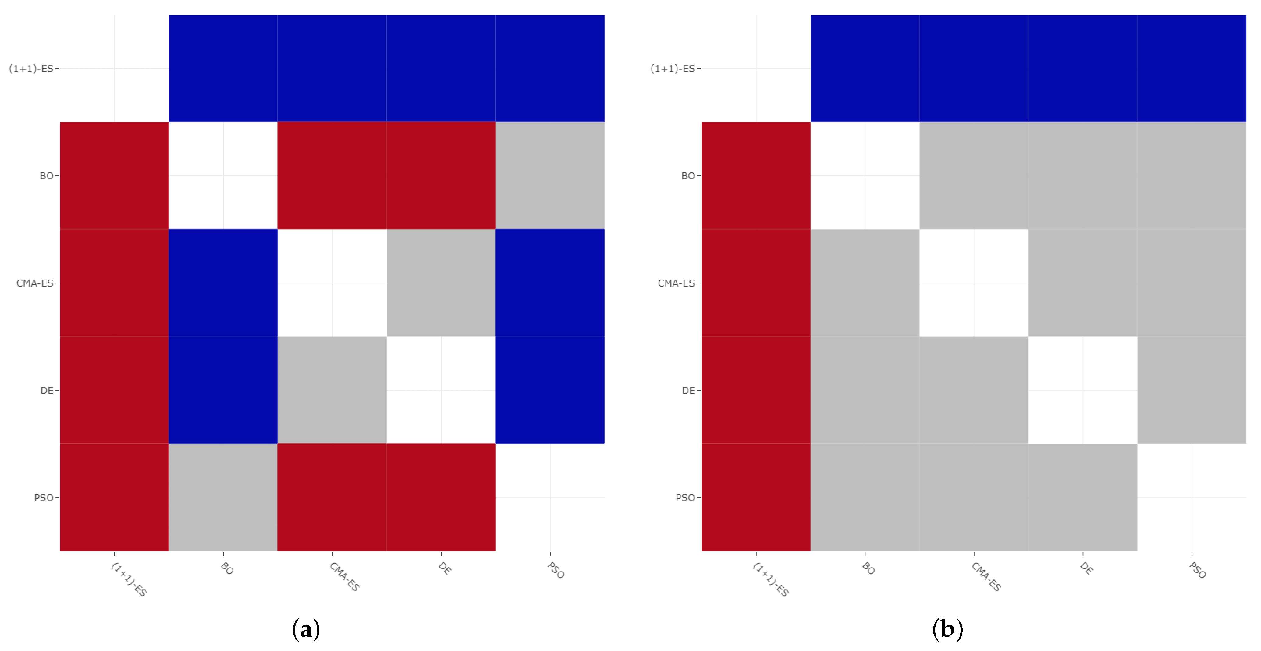
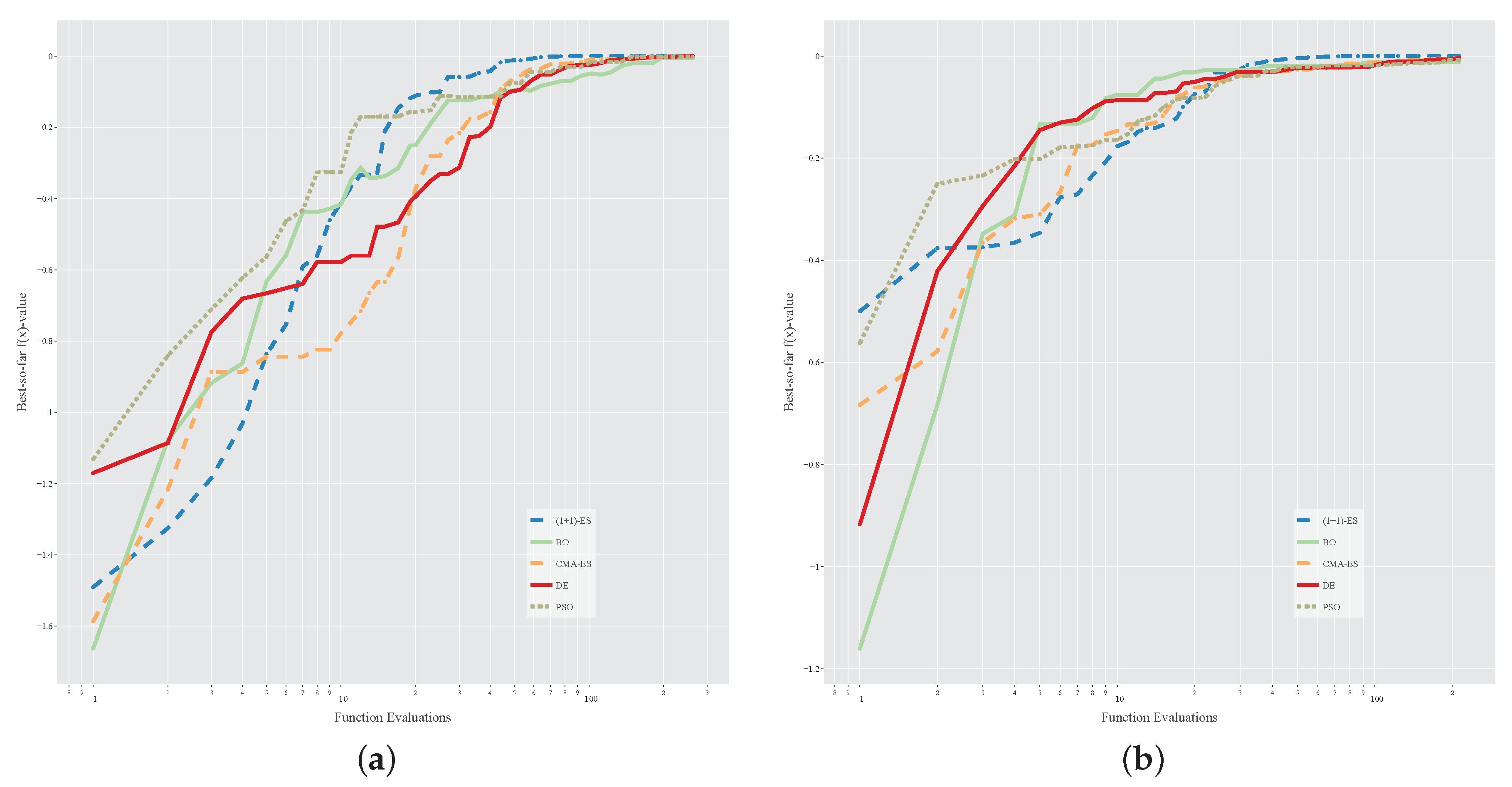
6. Experimental Results

We recorded final fitness values and corresponding positions in the search space from each run of the five selected meta-heuristics, thus allowing for statistical analysis of the optimisation results.

Table 1. Experimental results for the case study 1 river ‘Paglia’. For any meta-heuristic, the table provides the average, minimum, maximum and standard deviation of the fitness values observed at the end of all the 25 executions. For the standard method, which is deterministic, only one result is provided.

Algorithm	Final Fitness Values for the River Paglia
	Average	Minimum	Maximum	St.Dev.
(1 + 1)-ES	<10${}^{-\mathbf{5}}$	0	0.00005	<10${}^{-\mathbf{5}}$
DE	0.00147	0.00004	0.00665	0.00211
CMA-ES	0.00167	0.00013	0.00355	0.00139
BO	0.01364	0.00538	0.02898	0.00807
PSO	0.03719	0.00199	0.08304	0.03013
Std Method	1.63000

and

Table 2. Experimental results for the case study 2 river ‘Aniene’. For any meta-heuristic, the table provides the average, minimum, maximum and standard deviation of the fitness values observed at the end of all the 25 executions. For the standard method, which is deterministic, only one result is provided.

Algorithm	Final Fitness Values for the River Aniene
	Average	Minimum	Maximum	St.Dev.
(1 + 1)-ES	$\mathbf{0}.\mathbf{00003}$	0	0.00021	$\mathbf{0}.\mathbf{00006}$
DE	0.00362	0.00020	0.01190	0.00333
CMA-ES	0.00431	0.00051	0.01572	0.00442
PSO	0.00815	0.00048	0.01770	0.00532
BO	0.01212	0.00085	0.02762	0.00914
Std Method	1.78000

report the results for the Paglia and Aniene rivers respectively and display the average final fitness value, the minimum and maximum final fitness values, and the standard deviation obtained from the 25 executions of each algorithm under study. Note that the algorithms are ordered by increasing average fitness and the best results are denoted in boldface. Moreover, the last line of these tables shows the fitness value achieved with the deterministic standard methodology, described in Section 3.1, for further comparison.

From a quick inspection of Table 1 and Table 2, one can immediately notice that all the five meta-heuristics largely outperform the standard method, which is outperformed also if only the worst run is considered. Since the fitness values provided in the tables are the estimation errors in meters, the accuracy gain obtained by the proposed automatic methodology is of more than 1.5 m with respect to the standard approach in both the case studies, even considering the worst execution of the less effective meta-heuristic.

Regarding the results achieved by the five meta-heuristics, it is interesting to note that (1 + 1)-ES clearly outperforms all the other competitors. A possible reason for this is that the small budget of evaluations allowed—due to the intrinsic complexity of the fitness function—tends to favour trajectory-based algorithms, as (1 + 1)-ES is, to populationbased ones, as the other four meta-heuristics may be considered. Besides, the worst error obtained by execution of (1 + 1)-ES is of just 0.021 cm—in the Aniene case study, see Table 2–, thus making (1 + 1)-ES the algorithm to go for practitioners that want to consider our methodology for future works in flood analysis.

Moreover, for the purposes of the meta-heuristic research field, we also analyse the effectiveness of all the five competitor meta-heuristics. With this aim, the pairwise comparisons among the results of the meta-heuristics provided in Table 1 and Table 2 were statistically validated by means of the Kolmogorov-Smirnov (KS) statistical test [54]. Hence, by considering a significance level of 0.01, the results of the KS tests carried out are depicted in Figure 7a,b for, respectively, the river Paglia and the river Aniene. Each figure is a heatmap where a red square is used to indicate that the corresponding column-algorithm significantly outperforms the corresponding row-algorithm; a blue square means that the row-algorithm is significantly better than the column-algorithm; a grey square is used if there is no statistical difference between the two algorithms.

Figure 7a,b clearly confirm that (1 + 1)-ES significantly outperforms all the other competitors. Regarding the other comparisons, a distinction must be made between the two case studies. For the river Aniene—see Figure 7b—DE, CMA-ES, PSO and BO do not show significant differences in terms of effectiveness, while there are few differences in the case study Paglia—see Figure 7a. This is possibly due to the larger dimensionality of the second case study ($d=120$ vs. $d=60$) which reduces the number of iterations performed by the four population-based algorithms—in the allotted budget of computational time–, thus preventing them to show significant differences in the evolved population. However, in the case study Paglia—see Figure 7a–, DE and CMA-ES do not show significant differences between them, but both outperform PSO and BO.

The empirical probability density functions of the final fitness values obtained by the 25 executions of any single algorithm are depicted in the violin-plots of Figure 8a,b for, respectively, the river Paglia and the river Aniene.

These plots clearly confirm the main observation: (1 + 1)-ES is by a large amount the algorithm to go. Other observations are as follows:

• DE and CMA-ES look, in general, to be preferable to PSO and BO;
• BO is not competitive enough in both case studies and, in particular, its effectiveness deteriorates in the larger case study, probably because BO is not good enough for large dimensionalities (indeed, it is generally used to tune the few hyper-parameters of machine learning models [30]);
• regarding robustness, (1 + 1)-ES is clearly the most robust algorithm;
• the high variance for the results of the PSO algorithm may indicate the presence of a considerable amount of local optima in the fitness landscape, given that PSO is prone to prematurely converge to local optima [56];

Finally, Figure 9a,b depict the convergence behaviours of the five algorithms averaged over the 25 executions for, respectively, the river Paglia and the river Aniene.

It is interesting to observe that (1 + 1)-ES outperforms its population-based competitors (with population size equal to 30) after only 30 fitness functional evaluations, thus showing to be the most efficient and suitable for this problem. The convergence graphs also show that, with a larger budget, it is likely that both DE and CMA-ES will be able to match the same effectiveness of (1 + 1)-ES. However, since (1 + 1)-ES reaches a practically null error, there is no real need to increase the computational budget.

We can conclude this discussion by noting that the analyses provided take into account two different river traits and consider different amounts of cross-sections. In particular, this last characteristic influences the search space size of our methodology. Anyway, in both the case of studies—of 60 and 120 dimensions–, the (1 + 1)-ES algorithm allows a quicker convergence and larger robustness with respect to the other meta-heuristics. This is possibly due to (i) the small budget of computational time allowed for the task, and (ii) the trajectory-based nature of (1 + 1)-ES which does not require the ‘warmup time’ typical of population-based meta-heuristics. Therefore, we believe that even for different data in input, (1 + 1)-ES can be reasonably chosen as the algorithm to go with our methodology. However, this study does not take into account situations where the number of crosssections, so the dimensionality of the space, is very large. In such situations, two viable strategies are: (i) reduce the dimensionality by subsampling the cross-sections, (ii) increase the computational budget and give a try also to the population-based meta-heuristics DE and CMA-ES.

Finally, for the sake of completeness, we analysed the standard deviation of the estimated Manning’s values across the 25 different executions of the (1 + 1)-ES algorithm. These standard deviation values, for five selected cross-sections, are provided in

Table 3. Standard deviations of the Manning’s values obtained by the 25 executions of the (1 + 1)-ES algorithm for the case of study ‘river Paglia’. For the sake of readability, five cross-sections were reported, though the magnitude of the standard deviations is roughly the same for all the other cross-sections.

Cross Section	Std Dev. of the Manning’s Values for River Paglia
	Left Channel	Main Channel	Right Channel
1	0.007826	0.007999	0.009895
5	0.008051	0.007276	0.008452
10	0.007449	0.008903	0.006296
15	0.003794	0.008512	0.008731
20	0.006102	0.008623	0.008709

and

Table 4. Standard deviations of the Manning’s values obtained by the 25 executions of the (1 + 1)-ES algorithm for the case of study ‘river Aniene’. For the sake of readability, five cross-sections were reported, though the magnitude of the standard deviations is roughly the same for all the other cross-sections.

Cross Section	Std Dev. of the Manning’s Values for River Aniene
	Left Channel	Main Channel	Right Channel
1	0.006855	0.006383	0.006739
10	0.007071	0.006672	0.006709
20	0.006489	0.006073	0.006354
30	0.006764	0.006162	0.006629
40	0.008475	0.005951	0.007752

.

By recalling that the selected range for the roughness coefficients is $[0.02,0.2]$,Table 3 and Table 4 show that the standard deviations never overstep the $5\%$ of the selected range length. This means that the different executions of the considered algorithm converge to very similar Manning’s values, thus confirming the robustness of the algorithm. Similar behaviour has been observed also for the other four meta-heuristics.

7. Conclusions and Future Work

Hydraulic computational models are of paramount importance in preventing flood disasters. However, their accuracy heavily depends on the ability to estimate Manning’s roughness coefficients at multiple cross-sections of the considered rivers. These coefficients are influenced by the conformation of the channel and other channel’s features, thus making their calculation subject to uncertainty. This is why already existing deterministic Manning’s coefficients estimation methods show a low accuracy.

To avoid this problem, we propose a data-driven approach capable of returning optimal coefficients after minimising a purposely defined objective function that takes as input the coefficient values. These are used to run a flow simulation model to compute the (simulated) river depth at a given cross-section of the channel; finally, it compares the simulated river depth with the observed depth as measured at a gauge station deployed along the river.

Therefore, the designed objective function can be used as a fitness function to drive the search of meta-heuristic algorithms. In this work, we considered five well-known algorithms, i.e., the evolutionary strategy (1 + 1)-ES, DE, CMA-ES, PSO and BO.

The proposed methodology was used in two case studies: the river Paglia and the river Aniene, both located in Italy. The experimental results clearly show that our method largely outperforms the standard methodology usually adopted in the hydraulic computation literature, thus allowing us to build much more accurate hydraulic computational models.

The results from the comparative analysis among the five selected meta-heuristics have shown that, within the allocated computational budget (measured in fitness functional calls), the trajectory-based (1 + 1)-ES is the most effective algorithm. In line with the No Free Lunch Theorems for stochastic optimisation [57], this proves the importance of applying multiple and heterogeneous meta-heuristic approaches as a ‘universal’ solver does not exist and sometimes, as in this case, the simpler method can outperform the more complex and sophisticated ones.

Given the satisfactory results achieved in this piece of research, we recommend using this method and envisage further studies to improve upon it. A first improvement would be to validate our approach by considering a second hydraulic computational task, such as the case of a flow rate estimation [58]. This would let us analyse differences while performing this task with the estimated Manning’s coefficients, as in our approach, with respect to the traditional strategy. Another interesting future development would be to increase the number of gauge stations or, alternatively, the number of target values of water elevations deployed along the river cross-sections. We speculate that this might improve the performance of the current system. We also plan on modifying the objective function in an attempt to find more adequate ways for expressing the distance between simulated and measured depth vectors.

References

1. Ortigara, A.; Kay, M.; Uhlenbrook, S. A Review of the SDG 6 Synthesis Report 2018 from an Education, Training, and Research Perspective. Water 2018, 10, 1353. [Google Scholar] [CrossRef] [Green Version]
2. Koskinen, K.T.; Leino, T.; Riipinen, H. Sustainable development with water hydraulics-possibilities and challenges. Proc. JFPS Int. Symp. Fluid Power 2008, 2008, 11–18. [Google Scholar] [CrossRef] [Green Version]
3. Yusof, A.A.; Wasbari, F.; Zakaria, M.S.; Ibrahim, M.Q. Slip flow coefficient analysis in water hydraulics gear pump for environmental friendly application. In Proceedings of the IOP Conference Series: Materials Science and Engineering, Kazan, Russia, 25–27 September 2013; Volume 50, p. 012016. [Google Scholar]
4. Martınez-Vilalta, J.; Piñol, J.; Beven, K. A hydraulic model to predict drought-induced mortality in woody plants: An application to climate change in the Mediterranean. Ecol. Model. 2002, 155, 127–147. [Google Scholar] [CrossRef]
5. Zischg, A.P.; Mosimann, M.; Bernet, D.B.; Röthlisberger, V. Validation of 2D flood models with insurance claims. J. Hydrol. 2018, 557, 350–361. [Google Scholar] [CrossRef] [Green Version]
6. Kachiashvili, K.; Melikdzhanian, D. Software realization problems of mathematical models of pollutants transport in rivers. Adv. Eng. Softw. 2009, 40, 1063–1073. [Google Scholar] [CrossRef]
7. Pinar, E.; Paydas, K.; Seckin, G.; Akilli, H.; Sahin, B.; Cobaner, M.; Kocaman, S.; Atakan Akar, M. Artificial neural network approaches for prediction of backwater through arched bridge constrictions. Adv. Eng. Softw. 2010, 41, 627–635. [Google Scholar] [CrossRef]
8. Di Francesco, S.; Biscarini, C.; Manciola, P. Numerical simulation of water free-surface flows through a front-tracking lattice Boltzmann approach. J. Hydroinform. 2015, 17, 1–6. [Google Scholar] [CrossRef]
9. Di Francesco, S.; Biscarini, C.; Manciola, P. Characterization of a flood event through a sediment analysis: The Tescio River case study. Water 2016, 8, 308. [Google Scholar] [CrossRef] [Green Version]
10. Shen, D.; Jia, Y.; Altinakar, M.; Bingner, R.L. GIS-based channel flow and sediment transport simulation using CCHE1D coupled with AnnAGNPS. J. Hydraul. Res. 2016, 54, 567–574. [Google Scholar] [CrossRef]
11. Horritt, M.; Bates, P. Evaluation of 1D and 2D Numerical Models for Predicting River Flood Inundation. J. Hydrol. 2002, 268, 87–99. [Google Scholar] [CrossRef]
12. Violante, C.; Biscarini, C.; Esposito, E.; Molisso, F.; Porfido, S.; Sacchi, M. The consequences of hydrological events on steep coastal watersheds: The Costa d’Amalfi, eastern Tyrrhenian Sea. IAHS Publ. 2009, 327, 102. [Google Scholar]
13. Drake, J.; Bradford, A.; Joy, D. Application of HEC-RAS 4.0 temperature model to estimate groundwater contributions to Swan Creek, Ontario, Canada. J. Hydrol. 2010, 389, 390–398. [Google Scholar] [CrossRef]
14. Rodriguez, L.B.; Cello, P.A.; Vionnet, C.A.; Goodrich, D. Fully conservative coupling of HEC-RAS with MODFLOW to simulate stream–aquifer interactions in a drainage basin. J. Hydrol. 2008, 353, 129–142. [Google Scholar] [CrossRef]
15. Xing, Y.; Shao, D.; Yang, Y.; Ma, X.; Zhang, S. Influence and interactions of input factors in urban flood inundation modeling: An examination with variance-based global sensitivity analysis. J. Hydrol. 2021, 600, 126524. [Google Scholar] [CrossRef]
16. Atanov, G.A.; Evseeva, E.G.; Meselhe, E.A. Estimation of Roughness Profile in Trapezoidal Open Channels. J. Hydraul. Eng. 1999, 125, 309–312. [Google Scholar] [CrossRef]
17. Dooge, J.C. The Manning formula in context. In Channel Flow Resistance: Centennial of Manning’s Formula; Water Resources Publications, LLC.: Highlands Ranch, CO, USA, 1992; pp. 136–185. [Google Scholar]
18. Perry, B. Open-Channel Hydraulics. Science 1960, 131, 1215. [Google Scholar] [CrossRef]
19. Becker, L.; Yeh, W.W.G. Identification of parameters in unsteady open channel flows. Water Resour. Res. 1972, 8, 956–965. [Google Scholar] [CrossRef]
20. Di Francesco, S.; Zarghami, A.; Biscarini, C.; Manciola, P. Wall roughness effect in the lattice Boltzmann method. In Proceedings of the AIP Conference. American Institute of Physics, 11th International Conference of Numerical Analysis and Applied Mathematics-ICNAAM, Rhodes, Greece, 21–27 September 2013; Volume 1558, pp. 1677–1680. [Google Scholar]
21. Kiczko, A.; Romanowicz, R.J.; Napiorkowski, J.J. A Study of Flow Conditions Aimed at Preserving Valuable Wetland Areas in the Upper Narew Valley Using GSA-GLUE Methodology. In Environmental Informatics and Systems Research; Hryniewicz, O., Studzinski, J., Romaniuk, M., Eds.; Shaker Verlag: Aachen, Germany, 2007. [Google Scholar]
22. Romanowicz, R.; Kiczko, A.; Napiórkowski, J. Stochastic transfer function model applied to combined reservoir management and flow routing. Hydrol. Sci. J.—J. Des Sci. Hydrol. 2010, 55, 27–40. [Google Scholar] [CrossRef] [Green Version]
23. Hall, J.; Manning, L.; Hankin, R. Bayesian calibration of a flood inundation model using spatial data. Water Resour. Res. 2011, 47. [Google Scholar] [CrossRef] [Green Version]
24. Romanowicz, R.; Beven, K. Dynamic real-time prediction of flood inundation probabilities. Hydrol. Sci. J. 1998, 43, 181–196. [Google Scholar] [CrossRef] [Green Version]
25. Becker, L.; Yeh, W.W.G. Identification of multiple reach channel parameters. Water Resour. Res. 1973, 9, 326–335. [Google Scholar] [CrossRef]
26. Boussaïd, I.; Lepagnot, J.; Siarry, P. A survey on optimization metaheuristics. Inf. Sci. 2013, 237, 82–117. [Google Scholar] [CrossRef]
27. Eiben, A.E.; Smith, J.E. Introduction to Evolutionary Computation; Springer: Berlin, Germany, 2003. [Google Scholar] [CrossRef]
28. Kennedy, J. Swarm Intelligence. In Handbook of Nature-Inspired and Innovative Computing: Integrating Classical Models with Emerging Technologies; Springer: Boston, MA, USA, 2006; pp. 187–219. [Google Scholar] [CrossRef]
29. Caraffini, F.; Santucci, V.; Milani, A. Evolutionary Computation & Swarm Intelligence; MDPI: Basel, Switzerland, 2020. [Google Scholar]
30. Frazier, P.I. A tutorial on bayesian optimization. arXiv 2018, arXiv:1807.02811. [Google Scholar]
31. Yeoh, J.M.; Caraffini, F.; Homapour, E.; Santucci, V.; Milani, A. A clustering system for dynamic data streams based on metaheuristic optimisation. Mathematics 2019, 7, 1229. [Google Scholar] [CrossRef] [Green Version]
32. Brunner, W.G. HEC River Analysis System (HEC-RAS); No. 147; US Army Corps of Engineers, Hydrologic Engineering Center: Davis, CA, USA, 1994.
33. Dubin, J.R. On gradually varied flow profiles in rectangular openchannels. J. Hydraul. Res. 1999, 37, 99–106. [Google Scholar] [CrossRef]
34. Beyer, H.G.; Schwefel, H.P. Evolution strategies—A comprehensive introduction. Nat. Comput. 2002, 1, 3–52. [Google Scholar] [CrossRef]
35. Storn, R.; Price, K. Differential Evolution—A Simple and Efficient Heuristic for global Optimization over Continuous Spaces. J. Glob. Optim. 1997, 11, 341–359. [Google Scholar] [CrossRef]
36. Caraffini, F.; Kononova, A.V.; Corne, D. Infeasibility and structural bias in differential evolution. Inf. Sci. 2019, 496, 161–179. [Google Scholar] [CrossRef] [Green Version]
37. Price, K.; Storn, R.M.; Lampinen, J.A. Differential Evolution: A Practical Approach to Global Optimization; Springer: Berlin/Heidelberg, Germany, 2006. [Google Scholar]
38. Brabazon, A.; O’Neill, M.; McGarraghy, S. Natural Computing Algorithms, 1st ed.; Springer: Berlin/Heidelberg, Germany, 2015. [Google Scholar]
39. Santucci, V. Is Algebraic Differential Evolution Really a Differential Evolution Scheme? In Proceedings of the 2021 IEEE Congress on Evolutionary Computation (CEC), Krakow, Poland, 28 June–1 July 2021; pp. 9–16. [Google Scholar]
40. Santucci, V.; Baioletti, M.; Di Bari, G.; Milani, A. A Binary Algebraic Differential Evolution for the MultiDimensional Two-Way Number Partitioning Problem. In Proceedings of the 2019 European Conference on Evolutionary Computation in Combinatorial Optimisation, Leipzig, Germany, 24–26 April 2019; pp. 17–32. [Google Scholar]
41. Caraffini, F.; Neri, F. A study on rotation invariance in differential evolution. Swarm Evol. Comput. 2019, 50, 100436. [Google Scholar] [CrossRef]
42. Santucci, V.; Baioletti, M.; Milani, A. An algebraic framework for swarm and evolutionary algorithms in combinatorial optimization. Swarm Evol. Comput. 2020, 55, 100673. [Google Scholar] [CrossRef]
43. Santucci, V.; Baioletti, M.; Di Bari, G. An improved memetic algebraic differential evolution for solving the multidimensional two-way number partitioning problem. Expert Syst. Appl. 2021, 178, 114938. [Google Scholar] [CrossRef]
44. Meunier, L.; Doerr, C.; Rapin, J.; Teytaud, O. Variance reduction for better sampling in continuous domains. In Proceedings of the 16th International Conference on Parallel Problem Solving from Nature, Leiden, The Nederlands, 5–9 September 2020; pp. 154–168. [Google Scholar]
45. Hansen, N.; Ostermeier, A. Completely Derandomized Self-Adaptation in Evolution Strategies. Evol. Comput. 2001, 9, 159–195. [Google Scholar] [CrossRef]
46. Caraffini, F.; Neri, F.; Picinali, L. An analysis on separability for Memetic Computing automatic design. Inf. Sci. 2014, 265, 1–22. [Google Scholar] [CrossRef]
47. Beyer, H.G.; Sendhoff, B. Covariance Matrix Adaptation Revisited—The CMSA Evolution Strategy. In Parallel Problem Solving from Nature—PPSN X; Rudolph, G., Jansen, T., Beume, N., Lucas, S., Poloni, C., Eds.; Springer: Berlin/Heidelberg, Germany, 2008; pp. 123–132. [Google Scholar] [CrossRef]
48. Hansen, N. The CMA Evolution Strategy: A Tutorial. arXiv 2016, arXiv:cs.LG/1604.00772. [Google Scholar]
49. Rapin, J.; Teytaud, O. Nevergrad—A Gradient-Free Optimization Platform. 2018. Available online: https://GitHub.com/FacebookResearch/Nevergrad (accessed on 1 September 2021).
50. Kennedy, J.; Eberhart, R. Particle swarm optimization. In Proceedings of the IEEE International Conference on Neural Networks, Perth, Australia, 27 November–1 December 1995; Volume 4, pp. 1942–1948. [Google Scholar]
51. Santucci, V.; Milani, A.; Caraffini, F. An optimisation-driven prediction method for automated diagnosis and prognosis. Mathematics 2019, 7, 1051. [Google Scholar] [CrossRef] [Green Version]
52. Rapin, J.; Bennet, P.; Centeno, E.; Haziza, D.; Moreau, A.; Teytaud, O. Open source evolutionary structured optimization. In Proceedings of the 2020 Genetic and Evolutionary Computation Conference Companion, Cancun, Mexico, 8–12 July 2020; pp. 1599–1607. [Google Scholar]
53. Gray, D.N.; Hotchkiss, J.; LaForge, S.; Shalit, A.; Weinberg, T. Modern languages and Microsoft’s component object model. Comm. ACM 1998, 41, 55–65. [Google Scholar] [CrossRef]
54. Hollander, M.; Wolfe, D.A.; Chicken, E. Nonparametric Statistical Methods; John Wiley & Sons: Hoboken, NJ, USA, 2013; Volume 751. [Google Scholar]
55. Kim, J.; Scott, C.D. Robust kernel density estimation. J. Mach. Learn. Res. 2012, 13, 2529–2565. [Google Scholar]
56. Larsen, R.B.; Jouffroy, J.; Lassen, B. On the premature convergence of particle swarm optimization. In Proceedings of the 2016 European Control Conference, Aalborg, Denmark, 29 June–1 July 2016; pp. 1922–1927. [Google Scholar]
57. Wolpert, D.; Macready, W. No free lunch theorems for optimization. IEEE Trans. Evol. Comput. 1997, 1, 67–82. [Google Scholar] [CrossRef] [Green Version]
58. Chhantyal, K.; Hoang, M.; Viumdal, H.; Mylvaganam, S. Flow Rate Estimation using Dynamic Artificial Neural Networks with Ultrasonic Level Measurements. In Proceedings of the 9th EUROSIM Congress on Modelling and Simulation, Oulu, Finland, 12–16 September 2016. [Google Scholar] [CrossRef] [Green Version]
Figure 1. DEM images displaying the cross-sections for the two rivers Paglia (a) and Aniene (b).
Applsci 11 10575 g001
Figure 2. Example of Tabulated Manning’s coefficients for Channels from [18].
Applsci 11 10575 g002
Figure 3. Satellite (a) and DEM (b) representations of the simulated overflow event.
Applsci 11 10575 g003
Figure 4. HEC-RAS visualisation of the of the cross section placed in the same position of the gauge station.
Applsci 11 10575 g004
Figure 5. Bird eye view of ‘Ponte Lucano’ and ‘Tomba dei Plauzi’ in Tivoli, showing the industrial and flood-prone downstream area of the river [retrieved from Google Maps 20 July 2020].
Applsci 11 10575 g005
Figure 6. HEC-RAS representation of the water surface elevation of the Aniene river after the simulation with optimised Manning’s n.
Applsci 11 10575 g006
Figure 7. Results of the Kolmogorov-Smirnov tests with significance level 0.01. A red entry means that column-algorithm is significantly better than row-algorithm; a blue entry means that row-algorithm is significantly better than column-algorithm; a grey entry means that there is no statistical difference between the algorithms. (a) Case study 1—River Paglia; (b) Case study 2—River Aniene.
Applsci 11 10575 g007
Figure 8. Empirical probability density functions of the final fitness values registered by the executions of each algorithm estimated using the Kernel Density Estimation methodology [55]. (a) Case study 1—River Paglia; (b) Case study 2—River Aniene.
Applsci 11 10575 g008
Figure 9. Average convergence graphs of the algorithms’ best-so-far (abscissa is in log-scale). (a) Case study 1—River Paglia; (b) Case study 2—River Aniene.
Applsci 11 10575 g009