
Damage Identification in Warren Truss Bridges by Two Different Time–Frequency Algorithms


1
Dipartimento di Ingegneria Meccanica, Politecnico di Milano, Via La Masa 1, 20156 Milano, Italy
2
Dipartimento di Ingegneria Industriale e dell’Informazione, Università degli Studi di Pavia, Via Ferrata 5, 27100 Pavia, Italy
*
Author to whom correspondence should be addressed.
Appl. Sci. 2021, 11(22), 10605; https://0-doi-org.brum.beds.ac.uk/10.3390/app112210605
Submission received: 8 October 2021
/
Revised: 26 October 2021
/
Accepted: 4 November 2021
/
Published: 11 November 2021
Abstract
:Recently, a number of authors have been focusing on drive-by monitoring methods, exploiting sensors mounted on the vehicle rather than on the bridge to be monitored, with clear advantages in terms of cost and flexibility. This work aims at further exploring the feasibility and effectiveness of novel tools for indirect health monitoring of railway structures, by introducing a higher level of accuracy in damage modelling, achieve more close-to-reality results. A numerical study is carried out by means of a FE 3D model of a short span Warren truss bridge, simulating the dynamic interaction of the bridge/track/train structure. Two kinds of defects are simulated, the first one affecting the connection between the lower chord and the side diagonal member, the second one involving the joint between the cross-girder and the lower chord. Accelerations gathered from the train bogie in different working conditions and for different intensities of the damage level are analyzed through two time-frequency algorithms, namely Continuous Wavelet and Huang-Hilbert transforms, to evaluate their robustness to disturbing factors. Compared to previous studies, a complete 3D model of the rail vehicle, together with a 3D structural scheme of the bridge in place of the 2D equivalent scheme widely adopted in the literature, allow a more detailed and realistic representation of the effects of the bridge damage on the vehicle dynamics. Good numerical results are obtained from both the two algorithms in the case of the time-invariant track profile, whereas the Continuous Wavelet Transform is found to be more robust when a deterioration of track irregularity is simulated.
1. Introduction
Railway bridges represent a widely spread key component [1] within the railway infrastructure system. Most of them were designed several decades ago, when loading conditions and traffic volumes were different from today [2,3]. As a consequence, maintenance activities on the oldest bridges are more challenging, and sometimes linked to the extension of their service life. Improved health monitoring systems can be a valuable means to undertake efficient maintenance activity [4].
Current and established bridge maintenance techniques, embedded into technical specifications, rely on visual inspections and, in particular cases, on dedicated measurement systems to be installed on the bridge.
Visual inspection is effective if clear protocols are followed, according to the typology of bridge, and its main drawback consists of the possible dependence of the outcome on the skill and the experience of the inspecting operators and on the position of the damage, especially if the location of damage is not easily accessible. During these inspections, a quantitative assessment of the bridge status is often not possible or is lacking. Moreover, the time interval between consecutive inspections may depend on the availability of personnel and on the possibility to interrupt the vehicle service on the infrastructure. To improve the effectiveness of the inspections, additional means are desirable, like additional diagnostic systems.
The general way to reveal the presence of a local failure in a structure requires the comparison of some measurable indexes calculated from raw data in the current condition and in a reference healthy condition. The follow-up of such evolution enables, in principle, to distinguish a damaged condition from a healthy one. Basically, there can be two ways to monitor the status of a bridge: the most straightforward is to place dedicated instrumentation [5] on the structure. This solution, that can be called a direct method, can be worthwhile in the case of the main bridges of high-speed lines, but it is not a feasible prospective for regional or national networks, due the large number of bridges and the high related costs [6]. On-site measurements require several sensors to be mounted on the structure, leading to a significant cost of installation and maintenance of the entire set-up.
In order to overcome the issues concerning direct methods, in the last two decades a significant number of researchers have investigated new methods relying on sensors mounted onboard the vehicle [7], rather than on the structure to be monitored. The idea of using an indirect approach for structural health monitoring (commonly named Drive-by Methods [1] for SHM) derived from [8] in which the authors proposed the extraction of bridge frequencies from the dynamic response of a passing vehicle. The fundamental concept behind these approaches is that structural damage causes a change in the mechanical properties of the bridge, and consequently a change in the dynamic behavior of the vehicle interacting with the structure. The bridge health status can then be extracted from the dynamic response measured on-board train, e.g., on the axle box, on the bogie frame and on the carbody. For the time being, drive-by methods have been mainly developed for highway bridges (both numerically and experimentally), but in fewer cases they have been applied to railways too (only numerical studies). A major concern about the practical validity of drive-by approach consists in the fact that the train response might be influenced not only by the bridge status, but also by other factors not related to the damage, like the level of track irregularities, a different dynamic response of the vehicle due to different passenger loads, or other uncertainties related the train speed variation and accuracy of its positioning with respect to the bridge.
They can be divided in two main categories 1: modal parameter-based and non-modal parameter-based methods. The former, consisting in the identification of bridge properties like natural frequencies [9,10,11], damping values [12] and mode shapes [13,14] based on the vehicle response, have been shown to be effective up to limited speeds (i.e., a maximum of 60 km/h), and in the first two cases not able to identify the exact location of a defect. The effectiveness of most of the modal parameter-based techniques was only demonstrated through numerical simulations, and their outcomes can be affected by environmental conditions like temperature, especially in the case of damping and natural frequencies [15,16,17]. Conversely, non-modal parameter-based methods do not explicitly seek the computation of bridge modal parameters, but rather focus on the bridge deflection under passing loads (e.g., apparent profile [18,19] or change of curvature [20,21]) or on the dynamic response of the vehicle crossing the bridge [22,23,24,25,26,27], which is also the method investigated in this paper.
Concerning bridge modelling, most of the mentioned papers adopt a simply supported beam representation considering mainly the vertical deflection. Hester and Gonzalez showed good outcomes when considering single force and a half-car vehicle model crossing a simply supported beam [28]; Bowe et al. [26] investigated a ballasted bridge modelled as a simply supported beam without any track irregularity profile, where the train was modelled as a half-car vehicle (10 DOFs). Fitzgerald et al. proposed a numerical study on the scour phenomenon [29], with a 2D vehicle model (10 DOFs) moving on simply supported beams, with several beams in series to represent a multiple-span bridge. In this latter work, the track irregularity profile is taken into account, by introducing a time-invariant profile which does not allow consideration of any degradation process in the track. The results demonstrated good performance in terms of damage detection for vehicle speeds up to 80 km/h.
In all the mentioned works, the Continuous Wavelet Transform is adopted to analyze the motion of the vehicle: the wavelet coefficients are evaluated separately on the vehicle accelerations resulting from the simulations of the damaged and of the healthy bridges, assumed as a reference condition. The wavelet coefficients related to the damaged and healthy condition are subtracted from each other, so that any peak in the absolute value of this difference is used as an index to reveal the presence of a damage in the bridge structure. In most of the previously mentioned papers, the bridge defect is modelled through an equivalent representation of the damage, consisting of a reduction in the flexural stiffness of one of the finite elements of the beam schematization.
The present paper, starting from the previously mentioned papers, investigates the feasibility of the drive-by method applied to the basic 3D example of a short span Warren truss bridge, which according to the authors’ knowledge has not been done before. These bridges can be subjected to different degradation processes affecting the structure, such as corrosion, ageing, crack-growth and beam connection deterioration. Damage affecting a single member may represent a critical event, and it can lead to an increase in the load on the adjacent elements, and in some cases to sudden failures of the whole structure [30].
Concerning this issue, the studies in [31,32] demonstrate how damage affecting different members can cause different effects on the global response of the structure.
The main objective of the paper is to examine the feasibility to detect the presence of a defect in a steel truss bridge, from the processing of the acceleration recorded on a bogie frame of the train. While in the real system the acceleration would be measured on the bogie frame, in this paper the acceleration is simulated considering the train travelling on the bridge. Simulations of train–track–bridge interaction are carried out by means of the software ADTreS [33]. Some steps forward with respect to the literature are considered:
- Use of a finer schematization of the bridge, so that it is possible to consider the individual damaged element, and not an equivalent representation as it is necessarily adopted for a simply supported beam model.
- The schematization considering all the main structural members also enables location of the damage and better reproduction of its influence on train dynamics, following the real path from the defect to the point of acceleration detection on the train.
- The track and its irregularity are included in the model, considering also track irregularity variation while comparing two different train runs.
The paper is organized as follows: Section 2 describes the bridge model and briefly recalls the vehicle models used for the simulation of the bridge/track/train interaction. The damage consideration and the way track irregularity is taken into account are described, outlining the simulation plan. Section 3 describes the algorithms exploited for the signal processing. Section 4 discusses the results obtained and compares the performances of the Continuous Wavelet Transform against the Huang-Hilbert Transform, when the level of track irregularity is changed between damaged and heathy scenarios. Final conclusions are drawn in Section 5.
2. Models for Numerical Simulations
2.1. Bridge Model
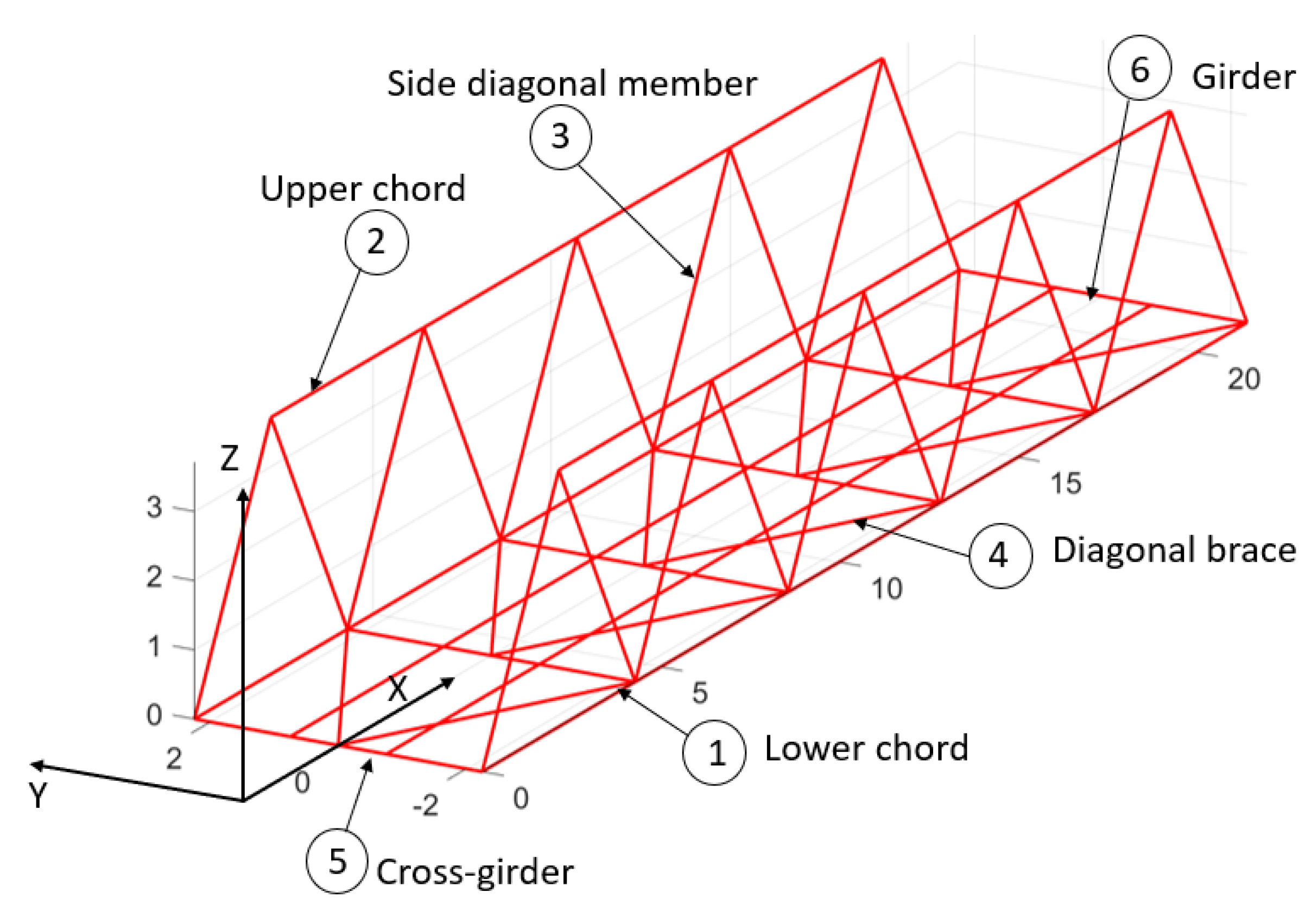
The bridge considered in the analysis is an open Warren truss bridge with a relatively short span (21.42 m) and single track. The bridge is modelled by means of beam finite elements, and the track is modelled by considering the two rails directly connected to the deck of the bridge through fastenings. The track system is intended to be with timber sleepers, which are considered as a rigid body in the present application. The section geometrical properties of the main structural members, shown in Figure 1, are collected in Table 1, while the resulting first bending and torsional natural frequencies of the span are gathered in Table 2.
Rail fastening are spaced along the track every 0.6 m, and reproduced by equivalent elastic springs and viscous elements, with the vertical stiffness of each fastening being equal to 0.95 × 10⁸ N/m. The scheme is completed with a portion of ballasted track located at each extremity of the bridge span.
2.2. Representation of the Damage
When dealing with steel truss bridges, one of the most likely-to-happen damage consists of a partial or total degradation of the fastenings in correspondence of the connections of the bridge elements. Chool-Wu Kim et al. [34] propose an experimental campaign on highway, in which a corrosion damage is reproduced by means of a fully severed diagonal element. The damage is caused artificially, but it is based on real observations performed on a Japanese truss bridge (i.e., Kisogawa bridge), according to [32,35]. In [35] Yamada shows that corrosion phenomena can lead to the total inefficiency of the connection between diagonal elements and lower chords on a steel truss bridge. A similar defect was observed, again in Japan on a steel truss bridge, precisely on the Honjo Ohashi bridge [32]. Following these researchers, two structural defects are considered in this paper, affecting, respectively, the connection of a diagonal member of the side wall (Section 2.2.1), and the deck in correspondence of the cross-girder connection with the lower chord (Section 2.2.2). The finite element schematization adopted following the main geometry of the real structure enables location of the damage in correspondence with the considered nodal connection.
2.2.1. Damage of Diagonal Elements in the Bridge Side Wall
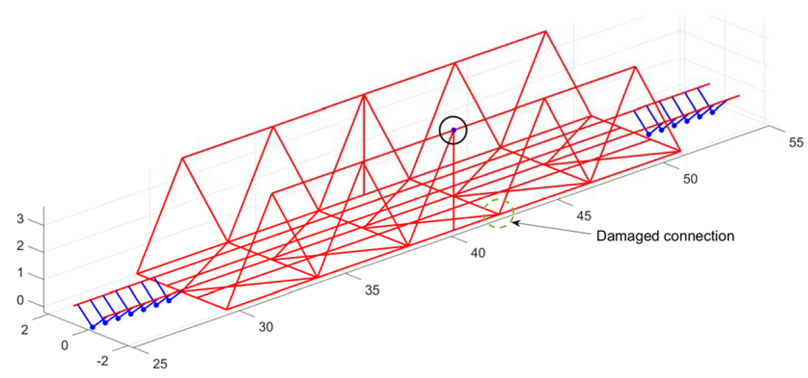
The first damage considered represents a degradation of the connection between a diagonal member and the lower chord. The structural components involved in the damage are highlighted with the dashed green circle shown in Figure 2. In case of total damage, the lateral element does not contribute to the global stiffness matrix of the bridge, since it does not transmit any axial action, but its mass still remains in the model, sustained by the upper connection. This damage can then be modelled by removing the diagonal element from the finite element model of the bridge, and by applying a concentrated inertia at the connection of the removed element with the upper chord (indicated with the black circled marker in Figure 2).
A less severe damage condition, which might occur in the case of partial degradation, is modeled through a reduction in the Young’s modulus of the damaged diagonal member in the FEM model. Clearly this way represents only the overall effect of the damaged connection on bridge dynamics. Three different defect entities have been considered, with a reduction in the Young’s Modulus equal to 30%, 50% and 70%, respectively, with respect to the nominal value.
For each damage type, the simulation plan is carried out by modelling the defect at different positions along the bridge span: this was done in order to assess whether and how the damage location affects the outcome of the detecting algorithms, either in terms of damage detection (i.e., false negative or false positive) or of accuracy in damage localization.
2.2.2. Damage on a Deck Cross-Girder
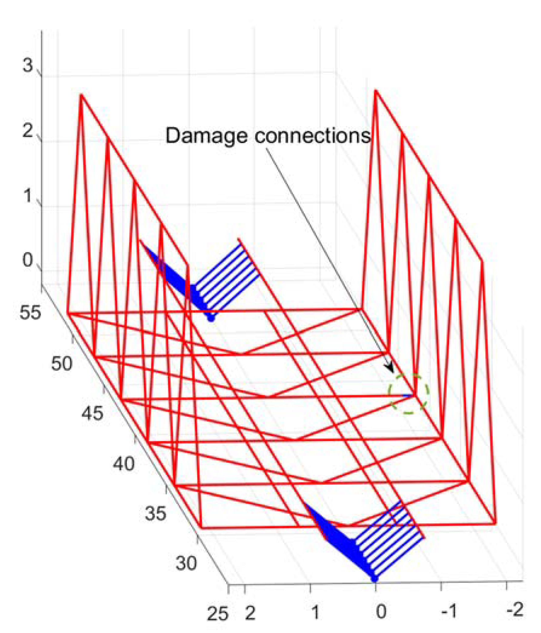
The second kind of damage simulated aims at representing a degradation of the connection between the lower chord and the cross-girders, as represented in Figure 3.
The beam fastenings might then be affected by bolts’ looseness and consequently by a reduction in the joint pressure and tightness, causing the bolts’ rods to touch with the inner surface of the related holes. As a consequence, due to stress concentration, some cracks may generate and propagate, further decreasing the strength of the joint.
This situation is modelled through an equivalent spring connecting the cross-girder to the lower chord, by substituting the last 200 mm of the deteriorated cross girder with the spring element. The springs are mainly described by two components, one in the z direction and a torsional one around the longitudinal axis x. Two damage entities have been considered in the simulation plan, namely a more severe one (with ) and a milder one (with ).
The first one represents more severe damage affecting the connection between the cross-girder and lower chord. The second one represents, on the other hand, damage at an earlier stage. In this last case, proper values of the stiffness components have been computed by assuming a reasonable relative vertical displacement (i.e., 1 mm) between the two ends of the spring in the presence of a static load of 160 kN, applied on the two rails. This displacement was chosen as a valid and reasonable representation of the bolt clearance.
2.3. Track Irregularity Profile
The presence of track irregularity, and its degradation in the long term, is a disturbing factor which affects the effectiveness of diagnostic methods based on the comparison of a damaged condition against a healthy reference condition. The damage effect might indeed be masked by the evolution of track irregularity.
For this reason, the paper investigates the stability of the outcome obtained by diagnostic algorithms when the accelerations simulated on-board of the vehicle are affected by different levels of track geometrical irregularity.
The irregularity profiles exploited are based on the power spectral density functions provided by report ORE B176 [36]. Different levels corresponding to different fractions of the original PSDs reported in the standard are considered to properly evaluate the robustness of the algorithms for increasing levels of irregularity.
Since the considered bridge is equipped with a non-ballasted track, a lower level of irregularity is set along the bridge span, compared to the two ballasted sections preceding and following the bridge span. This assumption is supported by the fact that, in the absence of permanent deformation of the bridge deck, the only enduring track displacements occurring along the bridge span may be those caused by the local degradation of the timber sleepers.
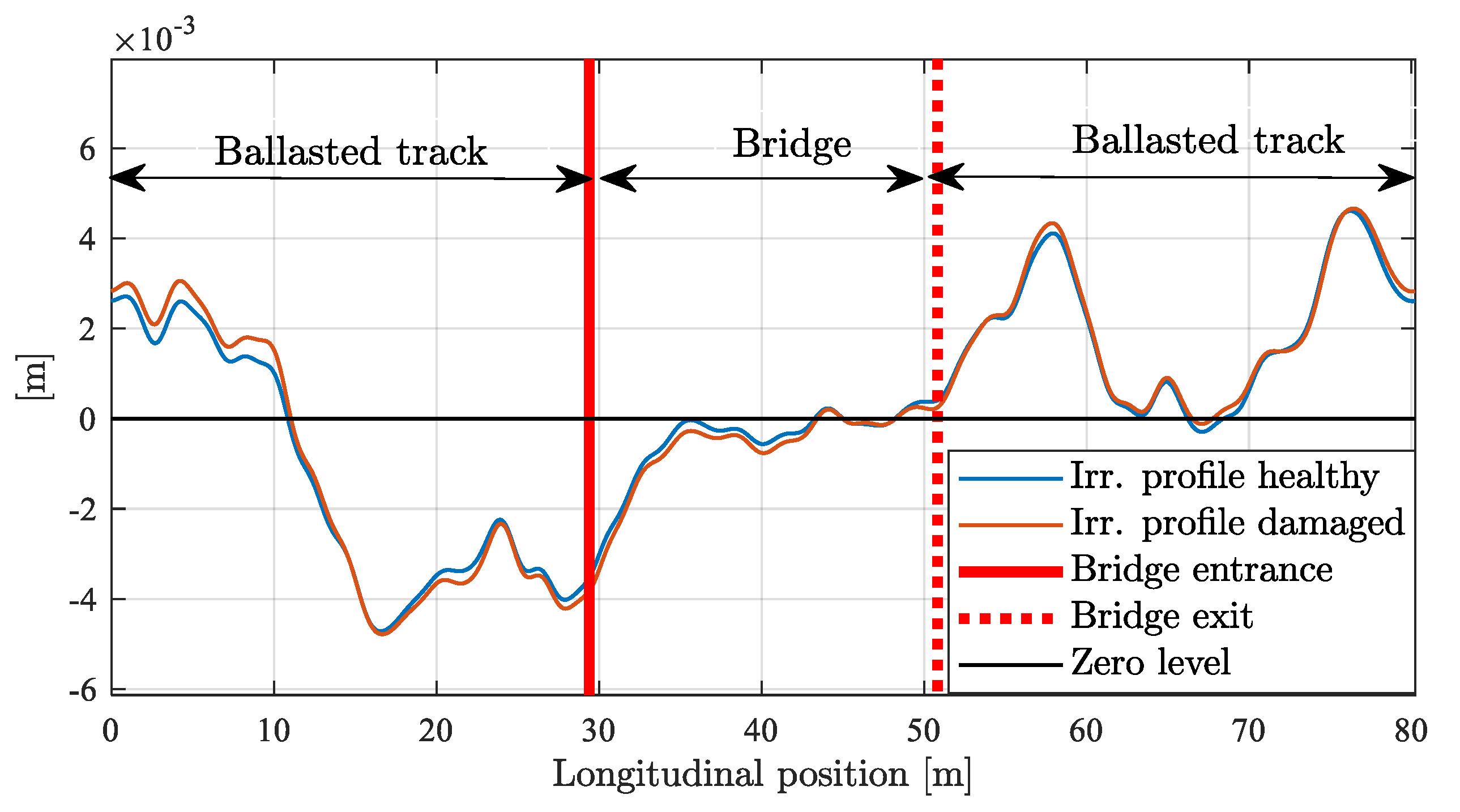
Two slightly different track profiles are adopted for the case of healthy and damaged bridge to account for a degradation occurring on the same track in a certain period of time. An example of the difference in track irregularity degradation adopted is reported in Figure 4: two different profiles can be observed, one exploited for the damaged bridge and one for the healthy bridge assumed as a reference.
The two profiles are described by two respective values of RMS that differ by 8%. This degradation can be assumed to be mild when dealing with a non-ballasted track [23], but it shall still be considered, since what is important is not simply the level but the associated derivative that causes variations of the vertical acceleration of the wheels.
2.4. Train Model
Two different train types are considered, respectively, featuring a standard two-bogie configuration for each carbody (the TSR train model) and by shared bogies between adjacent carbodies (the CSA train model). A scheme of the two trains is reported in reference [23] together with their dynamic and geometric parameters, not reported here for the sake of conciseness. The carbody and bogie frame have vertical, lateral, roll, pitch and yaw motions, while the wheelsets have vertical, lateral, yaw and roll motions.
The trains speed is in the range 80–140 km/h, corresponding to the real operating condition.
3. Numerical Algorithms for Signal Processing
This section presents the mathematical tools used to process the acceleration signals to be measured onboard. Two time-frequency domain algorithms are exploited, namely the Continuous Wavelet Transform (CWT) and the Huang-Hilbert Transform (HHT). The analysis is carried out by comparing the acceleration simulated in the case of the damaged bridge to the that corresponding to the healthy bridge. The need for comparison of two signals acquired during different train passages on the bridge implies, as a prerequisite, the adoption of precise train localization systems, in order to accurately localize the measurement along the track during the train run [37].
Bogie frame accelerations are considered for the analysis, under the assumption that the accelerometers to be used on the real train can be positioned on bogie frame on right and left side, in correspondence with the axle-boxes. It is worth reminding that the location of the accelerometers is of primary importance [23]: sensors mounted on the axle box require a higher full scale due to the higher level of acceleration they are subjected to, necessarily resulting in lower sensitivity. On the contrary, sensors mounted on the bogie frame can have a lower full scale and higher sensitivity, thanks to the filtering action provided by the primary suspension system.
3.1. Continuous Wavelt Transform (CWT)
The first procedure that is used for damage detection uses the Continuous Wavelet Transform (CWT) to extract useful indexes from the acceleration on the bogie frame.
The CWT [38] can exploit different waveforms to extract time-frequency information from the processed signals, as recalled in the following equation:
where τ represents the s time shifting value and s is defined as a scaling factor. Therefore, once the two parameters are set, represents a copy of the original mother wavelet scaled by s and centered around time τ. The wavelet coefficients indicate, along the time axis, if the shape associated to the defect is present in the time history of the acceleration on the bogie. The choice of a specific mother wavelet among those available in the literature can be made according to the features to be captured from the signal under analysis, which makes a CWT-based method versatile and flexible as a mean to extract a given signature in a time series. According to previous studies and to the oscillating pattern of the acceleration signals we dealt with in this work (see for example Figure 7, the choice fell on a real-valued Morlet Wavelet.
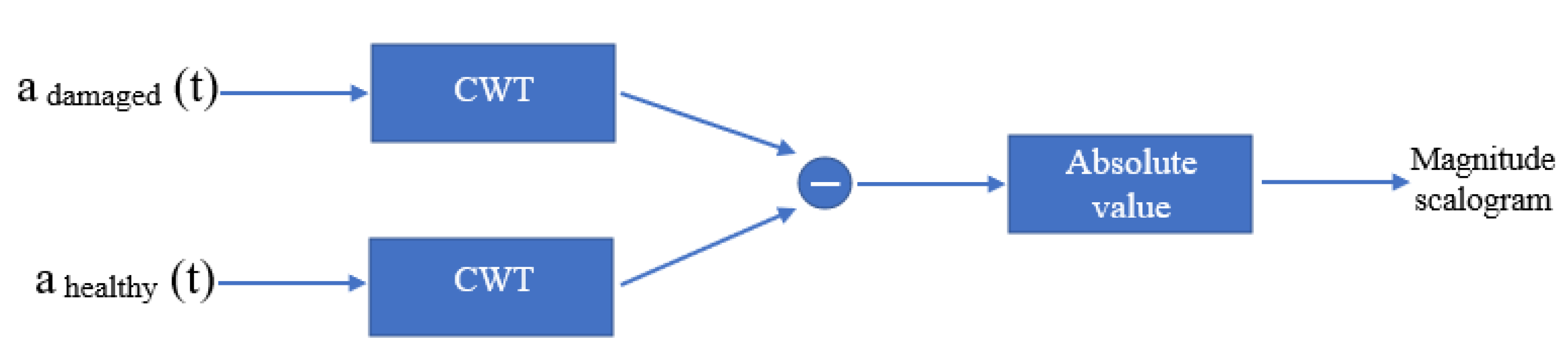
The scheme of the algorithm flow reported in Figure 5 shows that the CWT is applied separately to the accelerations measured in the case of the healthy and damaged bridge, respectively. Every time a train runs along a specific bridge, the wavelet coefficients of the current acquisition are evaluated and subtracted to the wavelet coefficient of the reference acquisition, corresponding to the healthy state of the bridge. The absolute value of the difference between the two series of CWT coefficients is then calculated: any peak pointing out a relevant difference between the current and the reference signal would indicate the presence of a defect and its position along the bridge span. The possibility to analyze, in a wayside server, data from different trains of an instrumented fleet would enhance the capability of the diagnostic system to filter outliers or false positives.
The comparison between the coefficients of the CWT calculated separately on the damaged and healthy time series, instead of calculating the CWT of the difference between the two time series, is expected to give some advantages in terms of lower sensitivity to extraneous effects not related to the damage.
This aspect will be investigated when considering the impact of different track irregularity in the damaged and healthy conditions.
3.2. Huang Hilbert Transform (HHT)
The second approach proposed in the paper uses the Huang-Hilbert Transform, which is generally adopted for the time-frequency analysis of non-stationary, nonlinear real time signals. It provides time-frequency information from the processed signal, through two steps:
- In the first step the empirical mode decomposition is applied, dividing the signal into different intrinsic mode functions (IMFs).
- In the second step the Hilbert transform is applied, from which the instantaneous frequency and the energy of the signal are obtained [39].
The plot of the Hilbert spectrum provides the time-frequency information about the processed signal. This procedure has been exploited in the diagnostics of railway infrastructure [40], while herein it is applied to drive-by methods for the condition monitoring of railway bridges.
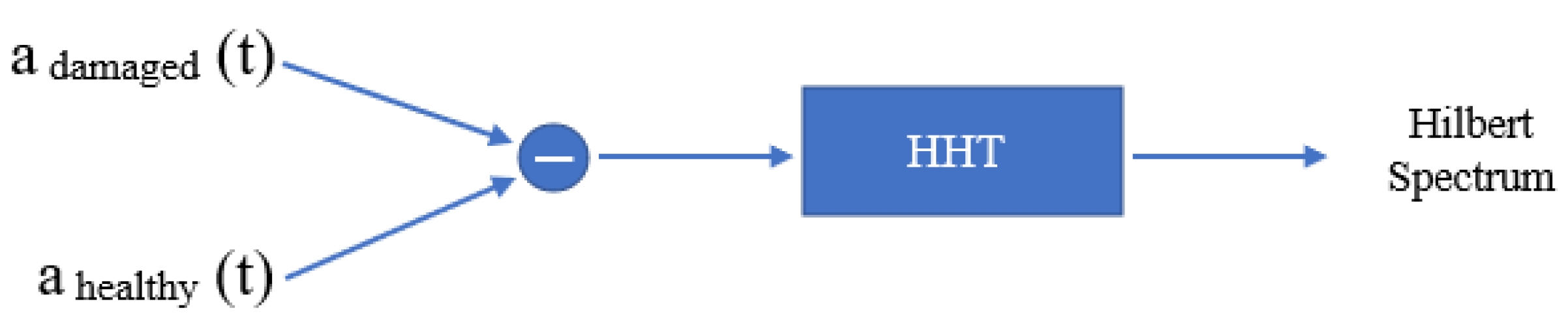
As shown in the flow chart of Figure 6, in this work the HHT is directly applied to the difference of the acceleration signals in the time domain: this is necessary to perform the IMF. A peak in terms of instantaneous energy, always associated to a specific frequency, allows detection of the presence of the damage and estimation of its position along the bridge.
4. Results
This section illustrates the results obtained by applying the two aforementioned procedures to the acceleration simulated on the leading bogie of the train. The outcomes achieved from the bogie accelerations corresponding to the side of the bridge damage are shown, with an increasing level of complexity of the simulations to evaluate the robustness of the two methods to disturbing factors.
As a reference example, the results obtained for the CSA train running at 100 km/h are reported, as well as all the remaining combinations of train and speeds leading to consistent results, as reported in the following sections.
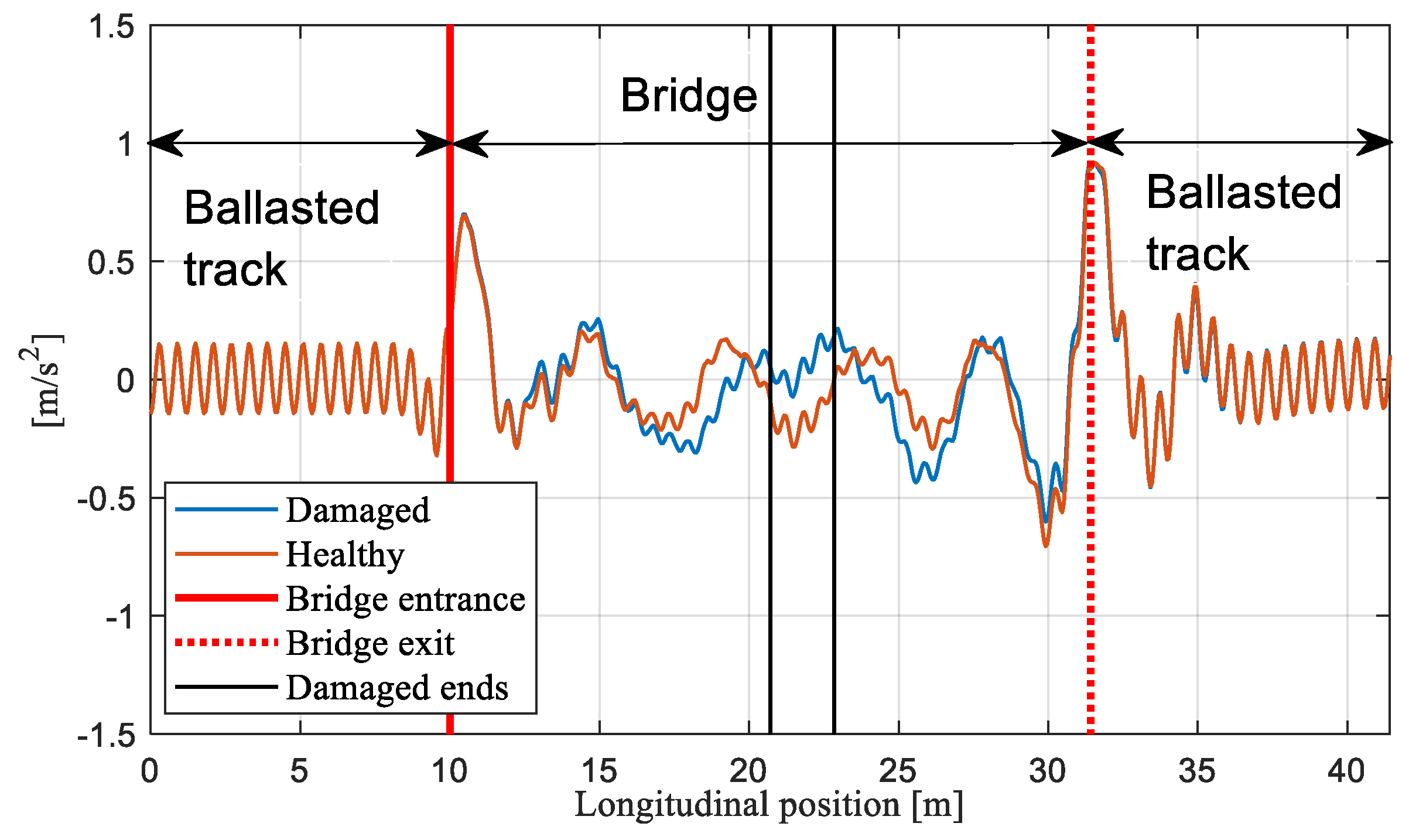
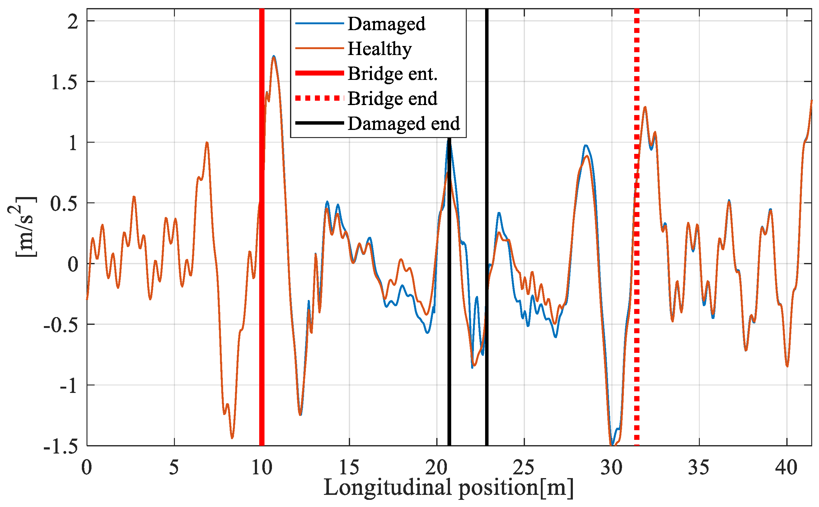
The first results presented illustrate the application of the procedures corresponding to the damage affecting the connection between the lower chord and a diagonal member of the bridge, as described in Section 2.2.1. Total damage on the second diagonal member of the third module of the bridge (see Figure 2) is considered, located at around mid-span. For clarity, in this introductory example no track irregularity is included in the simulation. Figure 7 compares the accelerations obtained on the leading bogie of the CSA train in case of a healthy and a damaged bridge, respectively. In the figure, as in all the following ones in this section, the two vertical black lines identify the two extremes of the damaged diagonal chord. The difference between the accelerations corresponding to the healthy and the damaged bridge is clearly visible in an area wider than the one directly affected by the defect. Although the defect is local, it extends its influence to a larger portion of the bridge.
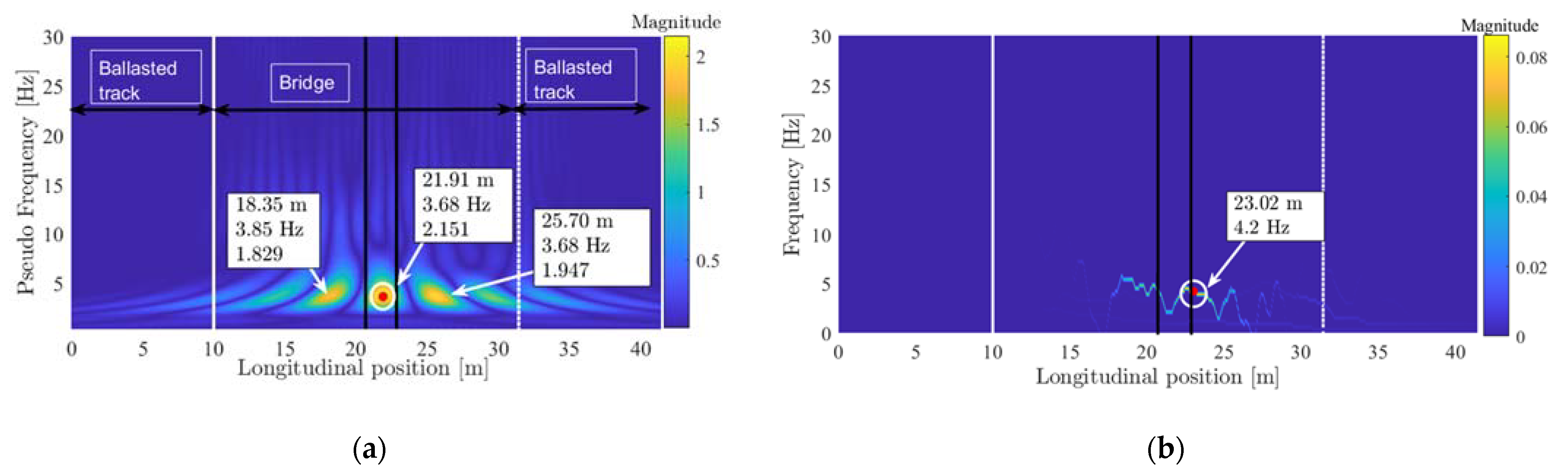
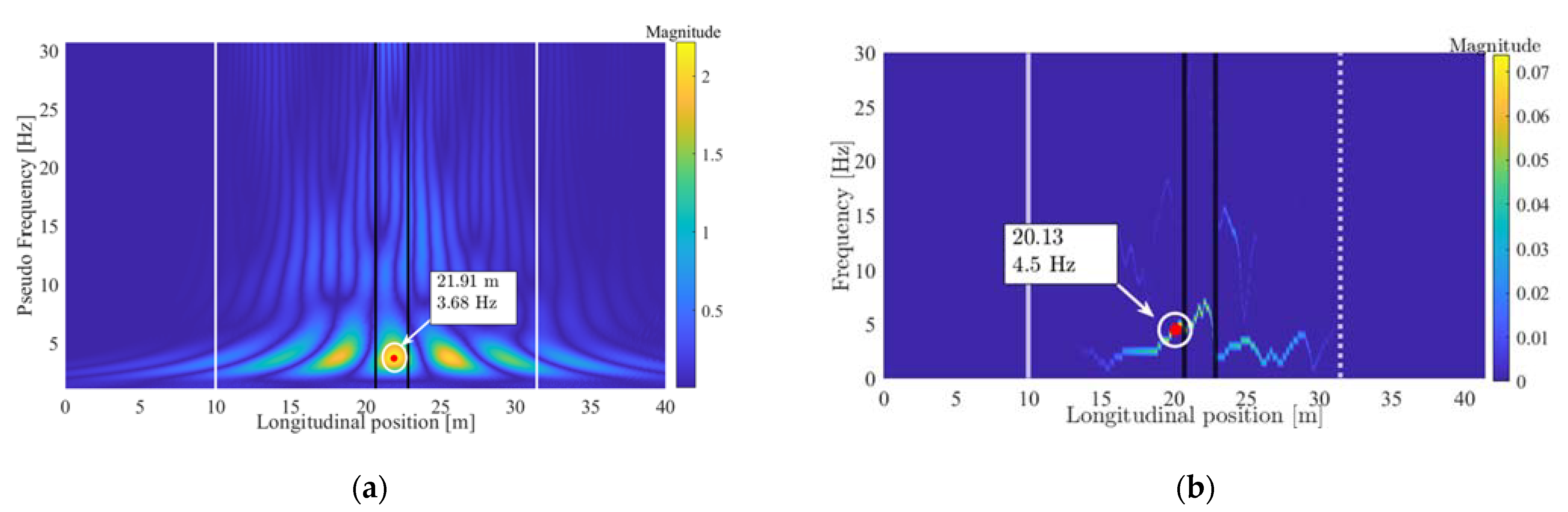
Figure 8a reports the position–frequency map of the difference of the CWT coefficients of the damaged and healthy condition, while the results of the HHT are reported in Figure 8b. In both the cases, the maxima of the index revealing the presence of the damage can identify the damaged region, although the HHT instantaneous energy peak falls at the right margin of the affected region.
The frequencies associated to the peaks detected by the two methods are rather similar (3.68 Hz and 4.2 Hz, respectively), so that the damage-related frequencies can be considered dependent on the nature of the damage itself rather than on the method used to detect its presence. The identified frequencies change proportionally with the train speed, so that they can be related to the extension of the region of influence of the damage on the bridge behavior.
The damage-related frequencies identified from the analysis do not change when an irregularity profile is added to the track. Figure 9 shows the accelerations on the leading bogie in case of the healthy and the damaged bridge with the same track profile (i.e., level 3, the highest level adopted).
Figure 10 reports the results obtained through the CWT (Figure 10a) and the HHT (Figure 10b). Again, the actual damage positions are correctly identified by the CWT and the HHT (the peak falls at the left margin of the damaged region), with damage-related frequencies (i.e., 3.68 Hz and 4.5 Hz, respectively) similar to those observed in Figure 9 without track irregularity. It can be therefore inferred that these appear to be related to the signature of the defect affecting the structure. As in the results of Figure 9, the HHT performs less precisely in locating the defect.
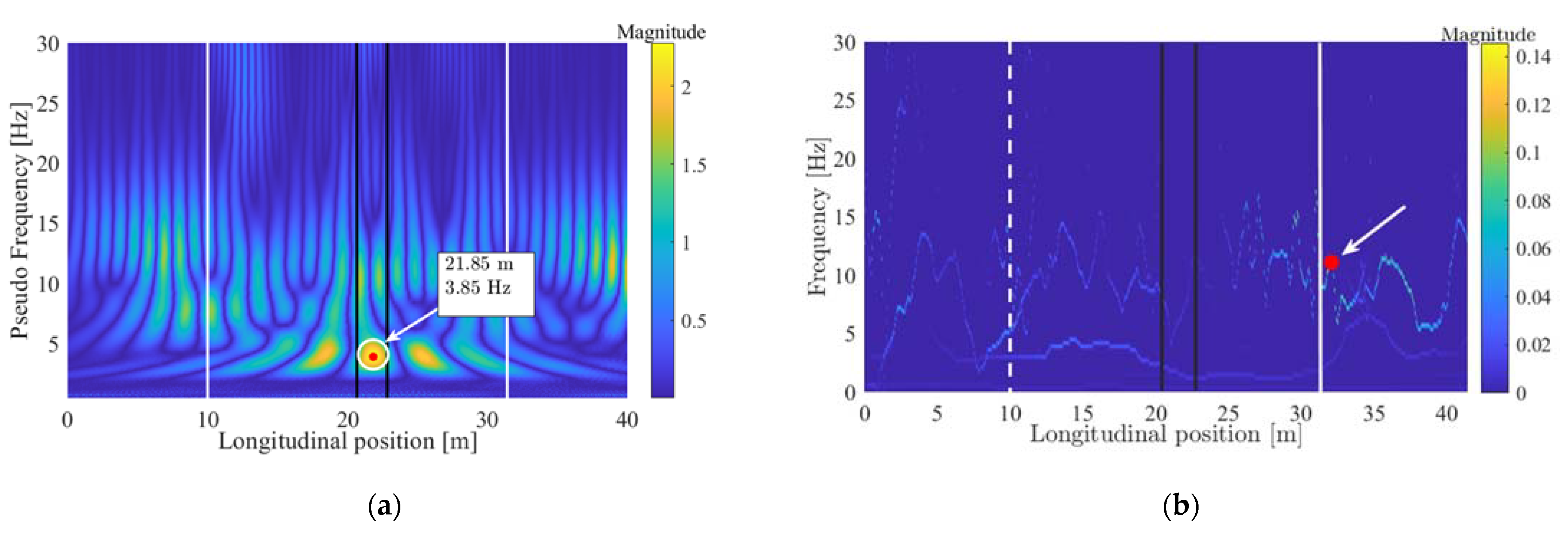
The better performances of the CWT compared to the HHT becomes more evident when the irregularity profile adopted for the damaged-bridge and the healthy-bridge simulations is slightly changed, to represent the track degradation with time which might occur between two consecutive observations. The difference in the irregularity profiles was of the same order as the ones reported in Figure 4: as stated before, the RMS of the two profiles differs by 8%. Figure 11 reports the results obtained by means of the CWT (Figure 11a) and the HHT (Figure 11b).
The CWT is still able to identify the damaged region, whereas the HHT results are affected by the change in the track profile which occurred in the two simulations. In the HHT result of Figure 11b, indeed, the maximum peak of instantaneous energy is detected outside the bridge span. The Continuous Wavelet Transform is therefore proven to be more robust to track profile changes. In this case, the damage-related frequency is similar to that presented in the previous cases (i.e., Figure 8a and Figure 10a), which confirms that it is actually related to the damage presence rather than to the track profile.
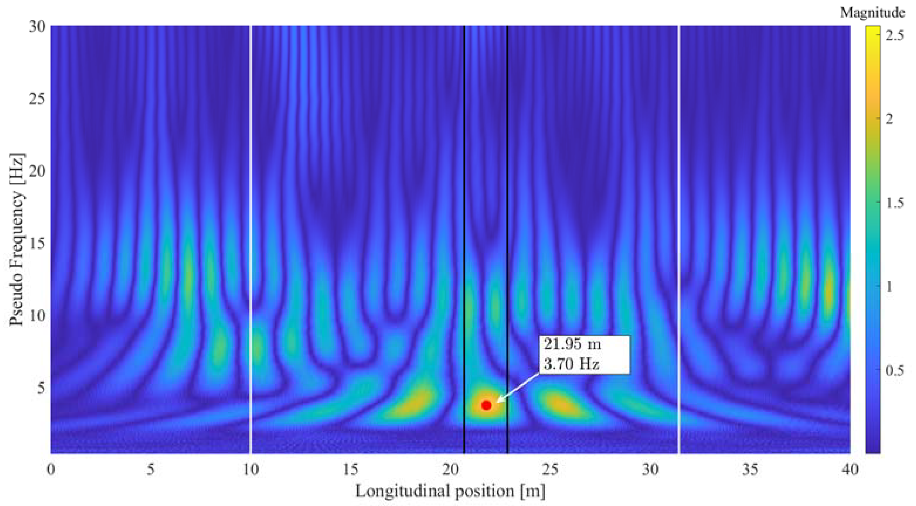
Furthermore, the CWT was also found to be robust to the presence of measuring noise, which was modelled in this work by means of a gaussian variable whose standard deviation is 10% of the RMS of the original signal. In fact, as shown in Figure 12, the CWT is still able to correctly identify the damage position across the bridge span, in the presence of a change in terms of track profile, and with the addition of measuring noise.
The results of the entire set of simulations carried out showed that, in the case of the time-invariant profile (and of course without the track irregularity profile), good identification performances are also obtained in the case of lower entity of the damage (i.e., partial damage modeled as described in Section 2.2.1), for both the CWT and HHT methods. However, when modelling a variation of the irregularity profile, even the effectiveness of the CWT method depends on the amount of change in the irregularity profile, and the severity of the damage. Only the total damage, representing a full disconnected joint, was detected for any tested change in track irregularity between the damage and healthy case simulation. Mild damages, on the contrary, are hidden even by low changes in the track profiles.
4.1. Influence of Damage Position
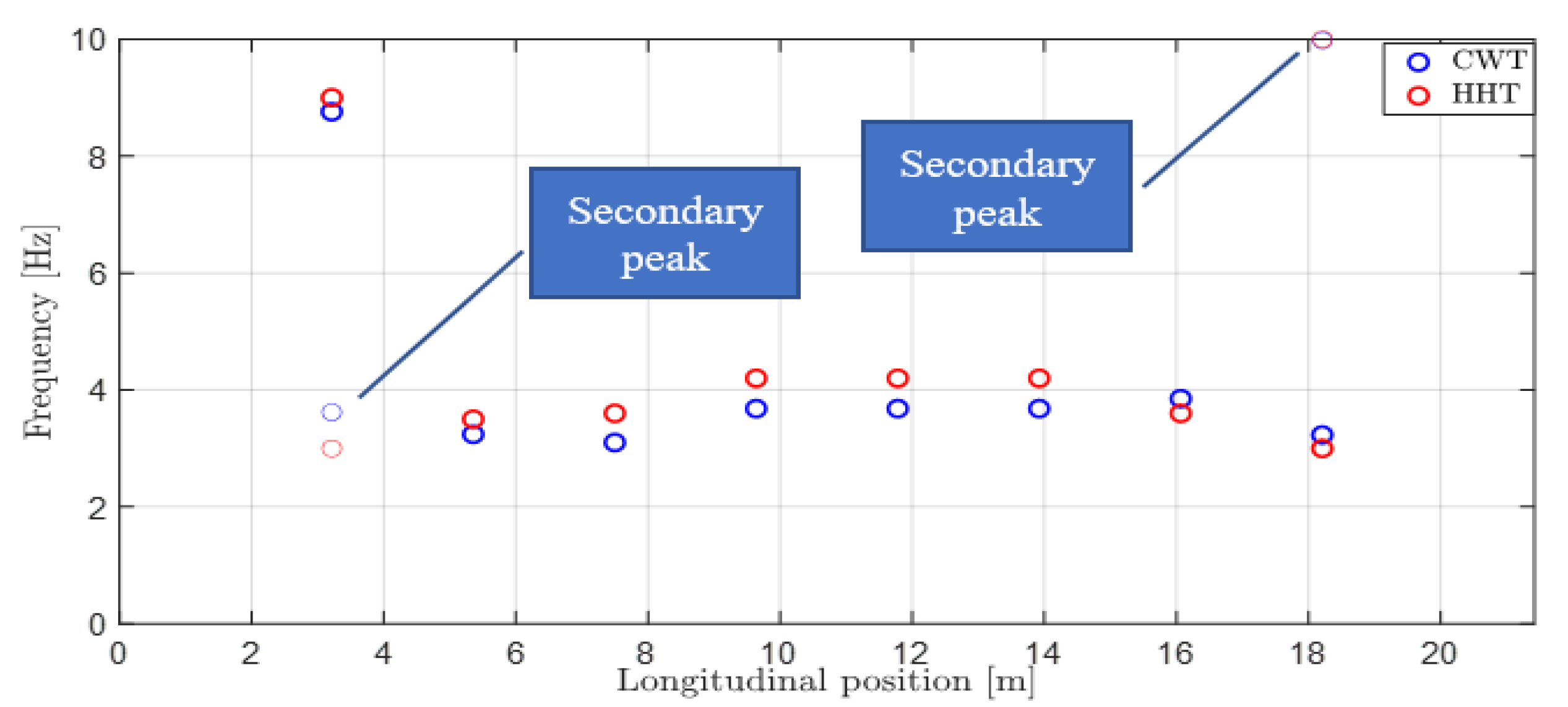
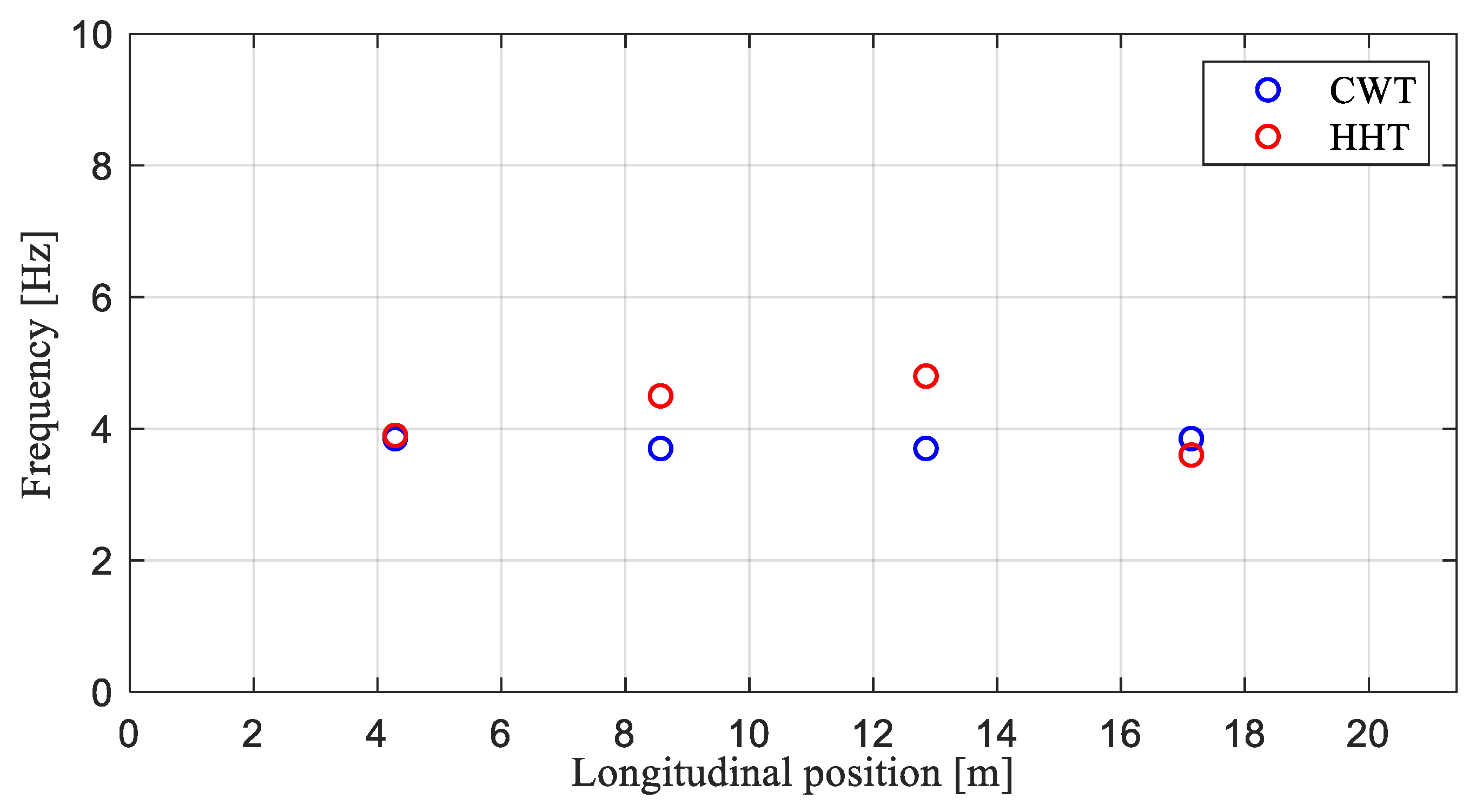
This section investigates the influence of the damage position on the results of the CWT and HHT diagnostic algorithms, without track irregularity. Figure 13 reports the damage-related frequencies as a function of the position of the defect along the bridge span. The results refer to the case of total damage of the diagonal chord.
The trends representing the damage-related frequency obtained from CWT and HHT show almost total agreement, enough to infer that the position of the damage along the bridge does not affect the coherence in terms of frequency information provided by the two different methods.
The damage-related frequency does not change significantly with the defect position, being in all cases close to the frequency values already given in Figure 8, Figure 10 and Figure 11. An exception was found in the points corresponding to the case in which the damage is located in the first module of the bridge (positioned at about 3 m), in which a dominant peak is visible at about 9 Hz. In this occurrence, the lower frequency peak is still present (represented with thinner circles), but it becomes a secondary peak compared to the main one at 9 Hz.
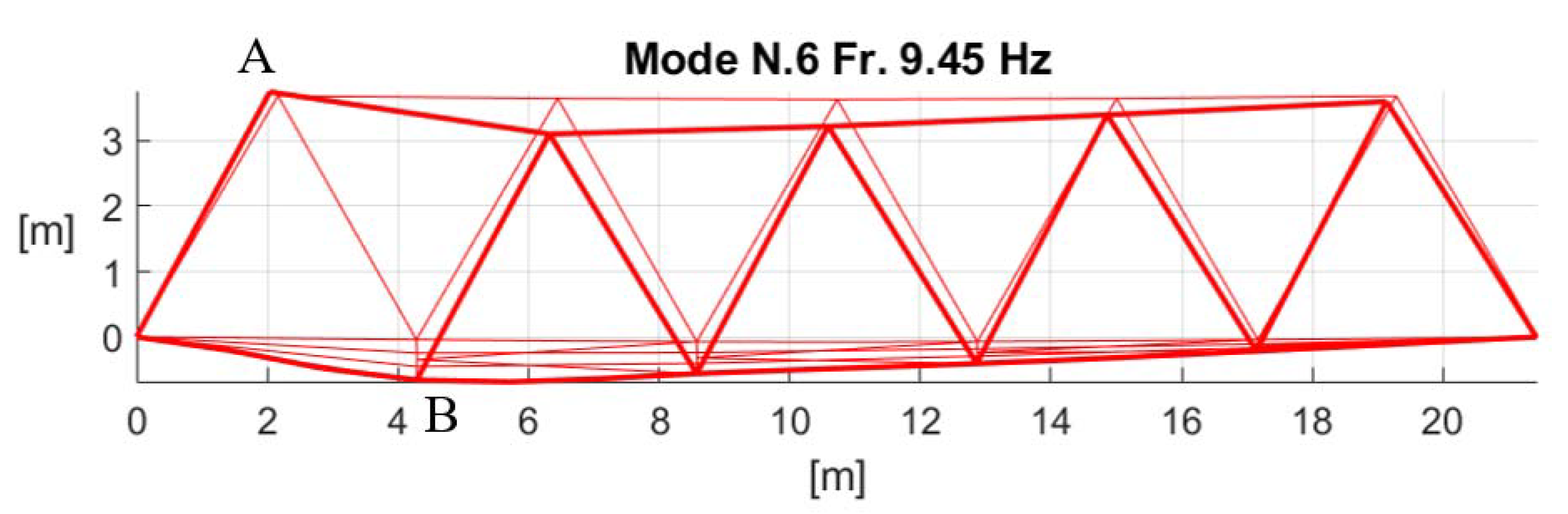
Modal analysis showed that a local mode of vibration at around 9 Hz, caused by the inefficiency of the diagonal chord, appears only in the cases in which the damage affects the first or last module in the bridge. On the other hand, it is not present when the damage is located along the other bridge modules; this may be due to the higher elastic energy which would occur for the local mode shape. This mode shape is represented in Figure 14.
The 9 Hz frequency peak is indeed also found in the CWT when the defect affects the last module, but in this case the dominant peak is the one at low frequency, which is therefore represented in Figure 13 (at the x-axis position of about 18 m): again, the secondary peaks (in terms of magnitudes) are represented with thinner circles.
The above-made observations point out that the damage-related frequency is generally due to the area of influence of the defect (being therefore dependent on train speed), but in some circumstances it can also be related to a mode of vibration of the structure, being therefore independent of train speed.
With the view to applying the drive-by method to a real bridge case, a preliminary modal analysis of the structure should therefore be carried out through FEM simulation of possible damaged configurations. This would allow estimation of the possible frequencies involved in the damaged structure, setting of a frequency range in the results of the CWT algorithm to maintain monitoring during the operation of the diagnostic system.
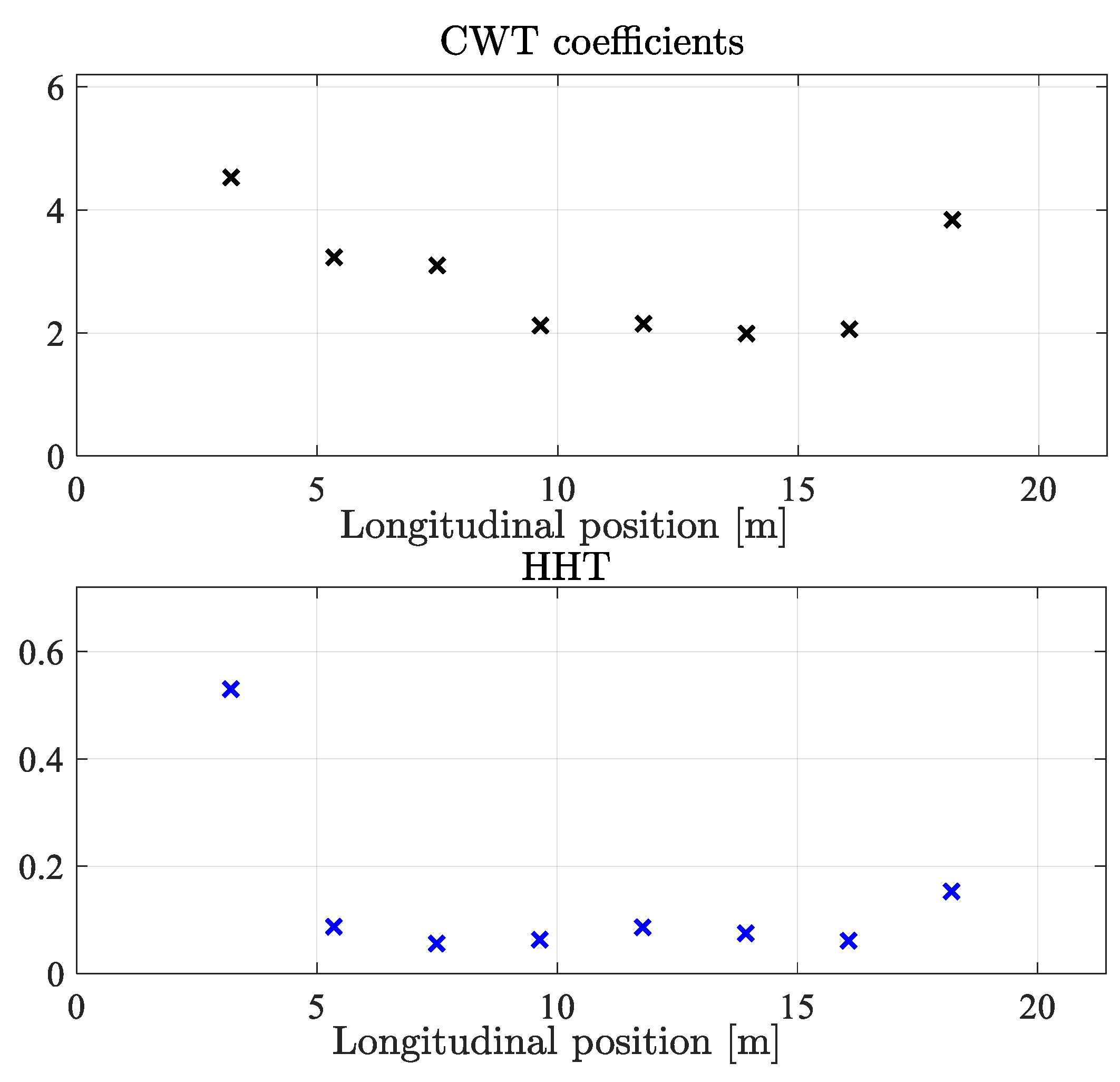
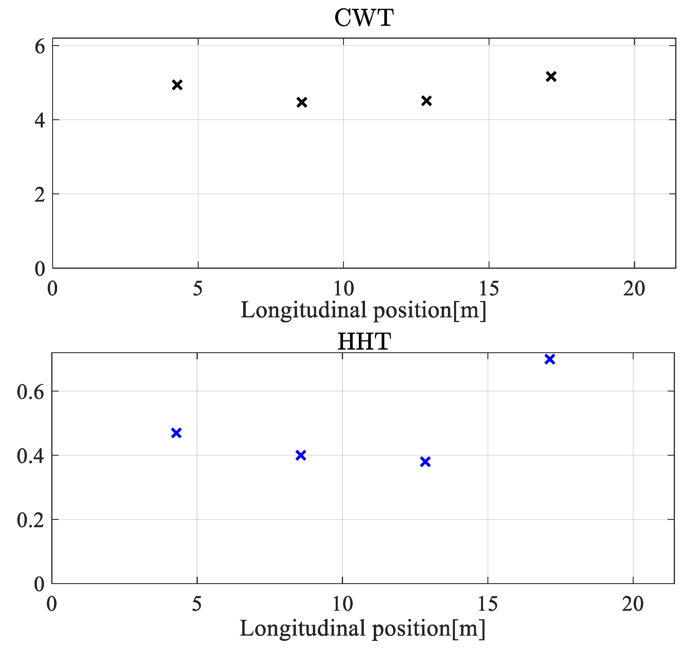
Figure 15 illustrates the magnitudes of the diagnostic indexes (i.e., CWT and HHT output) as a function of the location of the damage along the bridge span. It is possible to notice that defects occurring at the extremes of the bridge lead to higher magnitudes, if compared to the cases in which the damage affects the structure closer to mid-span. This is clearly visible in both the cases of damage affecting the first and the last module, and therefore not only in the case in which the 9 Hz normal frequency is involved. The reason is due to the fact that at the ends of the bridge the diagonal elements face higher shear forces, so the damage under analysis, involving a diagonal element of the side wall, leads to a more intense difference in the behavior of the bridge under the train passage. This is in agreement to what was observed by the authors in [31,32].
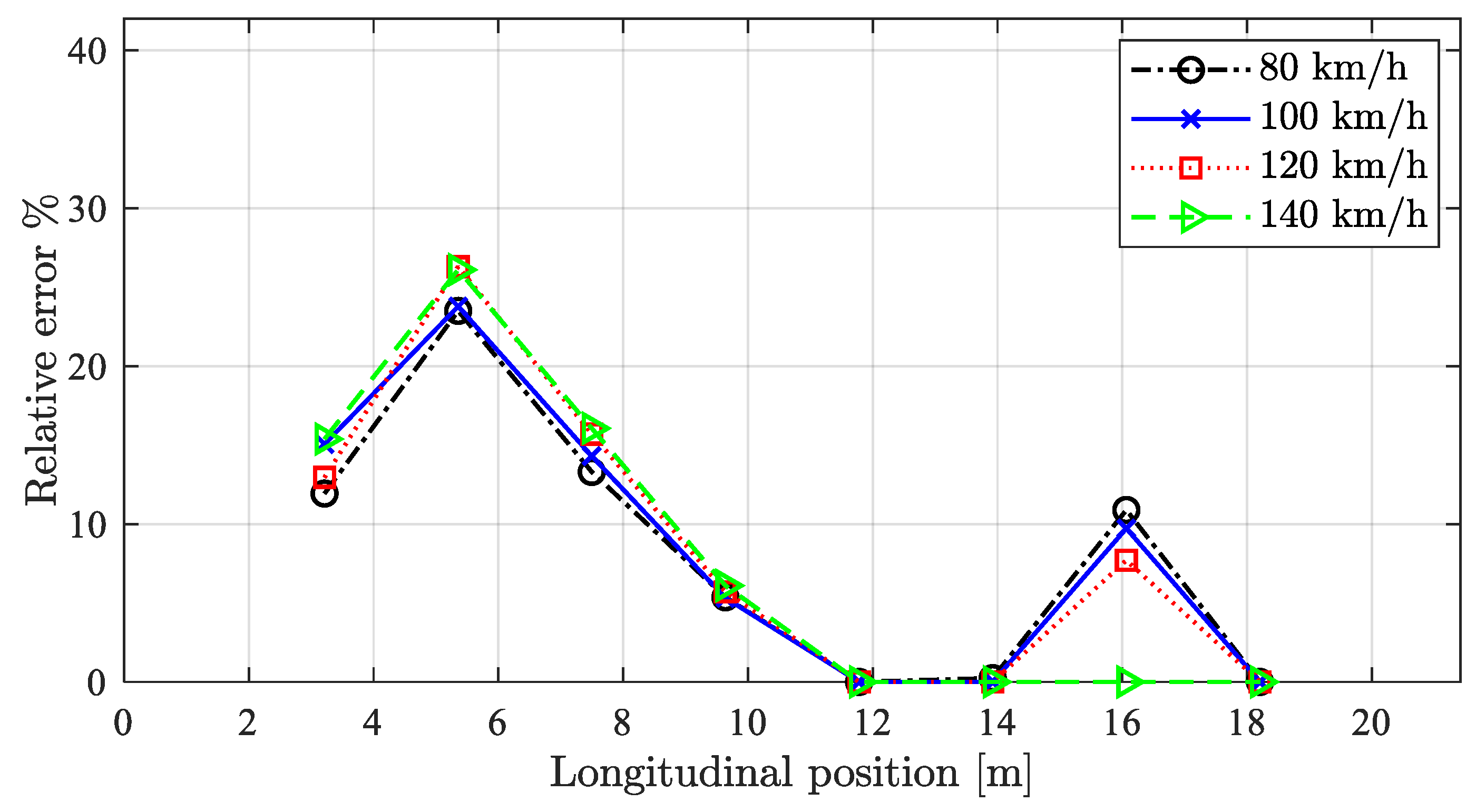
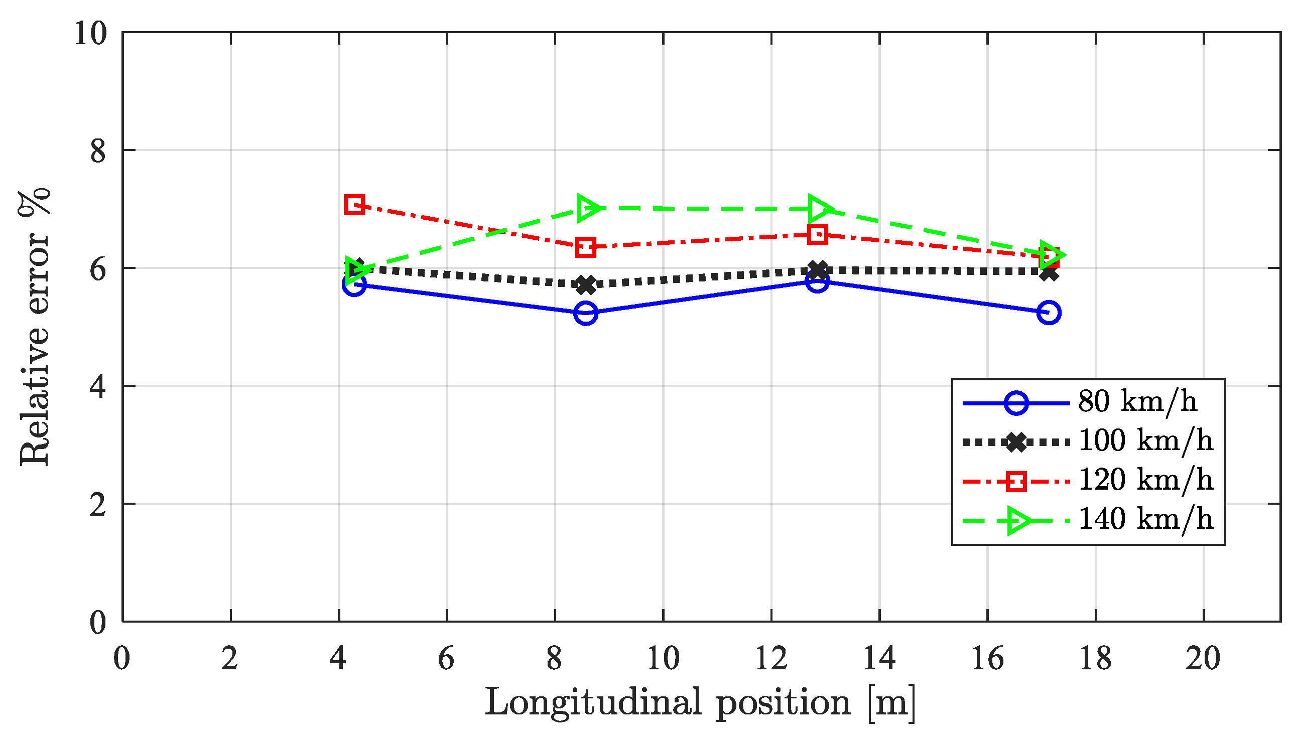
Finally, Figure 16 shows the trend of the relative identification error defined as the difference between the estimated damage position and the closest end of the region affected by the damaged diagonal member, divided by the bridge length. When the estimated damage position falls inside the currently deteriorated region, the relative identification error is null.
As for the train’s speed influence, Figure 16 reports the values of the relative identification error as a function of the position of the defect along the bridge span. The reported results, referring to the CWT algorithm, correspond to simulation cases in which a different track irregularity was adopted in the simulations of the damaged and healthy bridge.
The performances in locating the defect are rather good even in presence of a limited change of irregularity between the healthy and the damaged structure, and they are better when the damage is located close to or beyond the bridge mid-span.
4.2. Damage between Cross Girders and the Lower Chord
This section presents the simulation results corresponding to the second kind of bridge damage simulated, affecting the connection between the cross girders and the lower chord. This kind of defect was found to be more easily detectable by the proposed algorithm, being closer to the train wheel and therefore to the actual interaction point between the bridge structure and the vehicle. It was also detected in the case of mild defect, when changing the track irregularity between healthy and damaged cases.
Figure 17 illustrates the trend identified by the CWT and HHT algorithms in terms of damage-related frequency. The results refer to the CSA train travelling at 100 km/h, in the absence of track irregularity. Again, it is possible to state that the two time-frequency methods led to similar results in terms of frequency identification. The damage-related frequency is similar to the one identified for the previous kind of defect (Figure 13), meaning that the zones of influence of the two defects are rather similar. Moreover, the effect of the bridge damage on the first bending mode of vibration occurring at 16 Hz, is not large enough to be detected by the passing train.
Figure 18 is intended to investigate a possible dependence of the diagnostic indexes on the position of the damage along the bridge span. Compared to the previous damage scenario in Figure 15, it is possible to notice that for this defect the peak values seem to be less sensitive to damage position. On the other hand, the index magnitudes are generally higher, due to the fact that a defect affecting the cross-girder and the lower chord is closer to the points of interaction between the train and the bridge structure.
Finally, Figure 19 illustrates the identification performances of the CWT method as a function of the travelling speed and damage position rail vehicle. Since this type of defect is more local than the previous one, the relative identification error is redefined in Equation (3) as the difference in the estimated defect position and the actual deteriorated cross-girder position, over the length of the bridge:
The relative identification error identified in the case of damage between the cross girders and the lower chord is less dependent on the damage position, compared to the case of a defect affecting a diagonal element in the bridge side wall (see Figure 16). This may be due to the more direct coupling existing between what is sensed by the vehicle travelling on the bridge and the damage occurring on the cross-girder, rather than on the diagonal chord.
Before moving to conclusions section, it is important to remark that the relative identification error performances were computed differently due to the diverse nature of the two damages, in the sense that, while the diagonal element extends longitudinally (across the bridge span), the cross-girder, instead, is transverse to the bridge’s longitudinal axis.
5. Conclusions
This paper investigated the feasibility of drive-by methods for identifying the presence of damage in a Warren bridge, with single track, short span and a track with a wooden sleeper, which is a kind of bridge still present in regional railway lines. The study was carried out by means of the simulation of train/track/bridge interaction, considering specific defects consisting of loss of efficiency and till full failure of the connection between a generic diagonal member or cross-girder and the lower chord. The adoption of a model that reproduces the layout of the main structural members is a step forward in the field of drive-by methods.
Two different time-frequency algorithms, namely the Continuous Wavelet and the Huang-Hilbert transforms are adopted, both of them being based on the comparison between the acceleration signals measured on healthy and damaged bridge, respectively. In order to introduce disturbing effects which may affect the feasibility of this approach, a change of irregularity is assumed in the healthy and damaged bridge simulations, to represent a rail degradation occurring with time between consecutive runs on the bridge.
Two different damage scenarios are considered: the first one involves damage affecting the connection between the side wall diagonal members and the lower chord, while the second one regards the joint between the cross-girder and the lower chord. Different entities of the defect, different track profiles, travelling speeds and trains are considered in order to properly assess the capability of the algorithms to identify damage presence and position.
Regarding the two time-frequency algorithms the main outcomes can be summarized in the following points:
- Both the Continuous Wavelet (CWT) and the Huang-Hilbert (HHT) transforms show promising results in terms of damage identification in presence of a time-invariant track profile. This result might be of practical interest, since tracks directly linked to the bridge deck are likely to show a very contained degradation.
- The damage-related frequencies identified by the two algorithms are in agreement with each other. They mainly depend on the zone of influence of the defect and are therefore dependent on the train speed. However, for some specific cases, the presence of the defect can generate local modes of vibration, whose natural frequency can be detected by bogie accelerations in the case of the damaged bridge.
- The CWT is shown to be more robust than HHT to changes in the rail irregularity profiles. In fact, while the CWT also provides good results in the case of a varied irregularity profile in the cases of the healthy and the damaged bridge, the HHT becomes ineffective, not being able to identify the defect position with sufficient accuracy.
- When considering a time-variant irregularity, the effectiveness of the proposed method depends on the damage severity and entity. In fact, when dealing with partial damages, the exploitability of the approach is a trade-off between the damage level and the entity of the variation of the irregularity profile. In other words, time-variant track profiles may hide the damage component, especially in the case of mild damages.
- Another aspect that, according to authors, deserves to be further discussed is the effect that changes in terms of environmental condition could have on drive-by methods. It is true that the proposed indirect methods have the advantage of being non-modal parameter-based, and therefore they should be less affected by environmental changes as discussed in the introduction. Moreover, it is worth mentioning that the damage-related frequency (around 4 Hz) is far from the first bridge bending frequency (16 Hz). Anyway, a future outlook rising from this work could be represented by the investigation of the effect of environmental changes, such as temperature seasonality, on the vehicle-bridge interaction (VBI).
Furthermore, the two damage scenarios led to the following remarks:
- In the case of a damage scenario involving a deteriorated connection of the bridge side wall member with the lower chord, the defect identification performances are dependent on the location of the damage along the span. Moreover, a different bridge dynamic behavior was observed when the damage was located in the first or the last truss module.
- In the second damage scenario, in which the damage occurs on the cross-girder and is therefore more directly sensed by the vehicle travelling along the bridge, the magnitudes of the diagnostic indexes are higher. Both the index magnitudes and the damage positioning error are less sensitive to the position of the damage along the bridge span.
Despite some limitations, the results achieved in this paper encourage further research on the topic of drive-by methods, including more aspects related to real operation.
Author Contributions
The software used to carry out simulations was developed internally at the Department of Mechanical Engineering of Politecnico di Milano. It is named ADTReS. A.C. supervised all the works and drove the implementation of all the numerical models. L.B. developed the algorithms used for damage detection, while M.C. performed the analysis related to track irregularity. L.B. performed the simulations and data analysis, as part of his Master’s Thesis at Politecnico di Milano. The paper writing was mainly carried out by L.B and M.C. All authors have read and agreed to the published version of the manuscript.
Funding
This research received no external funding.
Conflicts of Interest
The authors declare no conflict of interest.
References
- Malekjafarian, A.; McGetrick, P.J.; Obrien, E.J. A Review of Indirect Bridge Monitoring Using Passing Vehicles. Shock. Vib. 2015, 2015, 286139. [Google Scholar] [CrossRef] [Green Version]
- Davis, S.L.; Goldberg, D. The Fix We’re in for: The State of Our Nation’s Bridges 2013; Transportation for America: Washington, DC, USA, 2013. [Google Scholar]
- Žnidarič, A.; Pakrashi, V.; O’Brien, E.; O’Connor, A. A review of road structure data in six European countries. Proc. Inst. Civ. Eng.—Urban Des. Plan. 2011, 164, 225–232. [Google Scholar] [CrossRef] [Green Version]
- Nielsen, D.; Raman, D.; Chattopadhyay, G. Life cycle management for railway bridge assets. Proc. Inst. Mech. Eng. Part F J. Rail Rapid Transit 2013, 227, 570–581. [Google Scholar] [CrossRef]
- Matsuoka, K.; Kaito, K.; Sogabe, M. Bayesian time-frequency analysis of the vehicle-bridge dynamic interaction effect on simple-supported resonant railway bridges. Mech. Syst. Signal Process. 2020, 135, 106373. [Google Scholar] [CrossRef]
- Yang, Y.-B.; Yang, J.P. State-of-the-Art Review on Modal Identification and Damage Detection of Bridges by Moving Test Vehicles. Int. J. Struct. Stab. Dyn. 2018, 18, 31. [Google Scholar] [CrossRef]
- Quirke, P.; Cantero, D.; Obrien, E.J.; Bowe, C. Drive-by detection of railway track stiffness variation using in-service vehicles. Proc. Inst. Mech. Eng. Part F J. Rail Rapid Transit 2017, 231, 498–514. [Google Scholar] [CrossRef] [Green Version]
- Yang, Y.-B.; Lin, C.; Yau, J. Extracting bridge frequencies from the dynamic response of a passing vehicle. J. Sound Vib. 2004, 272, 471–493. [Google Scholar] [CrossRef]
- Siringoringo, D.M.; Fujino, Y. Estimating Bridge Fundamental Frequency from Vibration Response of Instrumented Passing Vehicle: Analytical and Experimental Study. Adv. Struct. Eng. 2012, 15, 417–433. [Google Scholar] [CrossRef]
- Yang, Y.B.; Li, Y.C.; Chang, K.-C. Using two connected vehicles to measure the frequencies of bridges with rough surface: A theoretical study. Acta Mech. 2012, 223, 1851–1861. [Google Scholar] [CrossRef]
- Kim, C.-W.; Chang, K.-C.; McGetrick, P.J.; Inoue, S.; Hasegawa, S. Utilizing Moving Vehicles as Sensors for Bridge Condition Screening—A Laboratory Verification. Sens. Mater. 2017, 29, 1. [Google Scholar] [CrossRef] [Green Version]
- Curadelli, R.O.; Riera, J.D.; Ambrosini, D.; Amani, M.G. Damage detection by means of structural damping identification. Eng. Struct. 2008, 30, 3497–3504. [Google Scholar] [CrossRef]
- Zhang, Y.; Wang, L.; Xiang, Z. Damage detection by mode shape squares extracted from a passing vehicle. J. Sound Vib. 2012, 331, 291–307. [Google Scholar] [CrossRef]
- Obrien, E.J.; Malekjafarian, A. A mode shape-based damage detection approach using laser measurement from a vehicle crossing a simply supported bridge. Struct. Control. Health Monit. 2016, 23, 1273–1286. [Google Scholar] [CrossRef]
- Obrien, E.J.; Malekjafarian, A.; González, A. Application of empirical mode decomposition to drive-by bridge damage detection. Eur. J. Mech. A Solids 2017, 61, 151–163. [Google Scholar] [CrossRef] [Green Version]
- Fan, W.; Qiao, P. Vibration-based Damage Identification Methods: A Review and Comparative Study. Struct. Health Monit. 2011, 10, 83–111. [Google Scholar] [CrossRef]
- Qiao, P.; Cao, M. Waveform fractal dimension for mode shape-based damage identification of beam-type structures. Int. J. Solids Struct. 2008, 45, 5946–5961. [Google Scholar] [CrossRef] [Green Version]
- Quirke, P.; Bowe, C.; Obrien, E.J.; Cantero, D.; Antolin, P.; Goicolea, J.M. Railway bridge damage detection using vehicle-based inertial measurements and apparent profile. Eng. Struct. 2017, 153, 421–442. [Google Scholar] [CrossRef]
- Elhattab, A.; Uddin, N.; Obrien, E. Drive-by bridge damage monitoring using Bridge Displacement Profile Difference. J. Civ. Struct. Health Monit. 2016, 6, 839–850. [Google Scholar] [CrossRef]
- Obrien, E.J.; Martinez, D.; Malekjafarian, A.; Sevillano, E.; Otero, D.M. Damage detection using curvatures obtained from vehicle measurements. J. Civ. Struct. Health Monit. 2017, 7, 333–341. [Google Scholar] [CrossRef] [Green Version]
- Malekjafarian, A.; Martínez, D.; Obrien, E.J. The Feasibility of Using Laser Doppler Vibrometer Measurements from a Passing Vehicle for Bridge Damage Detection. Shock. Vib. 2018, 2018, 9385171. [Google Scholar] [CrossRef] [Green Version]
- Amerio, L.; Carnevale, M.; Collina, A. Damage Detection in Railway Bridges by Means of train on-Board Sensors: A Perspective Option. In The Dynamics of Vehicles on Roads and Tracks, Proceedings of the 25th International Symposium on Dynamics of Vehicles on Roads and Tracks (IAVSD 2017), Rockhampton, Australia, 14–18 August 2017; CRC Press: Boca Raton, FL, USA, 2017. [Google Scholar]
- Carnevale, M.; Collina, A.; Peirlinck, T. A Feasibility Study of the Drive-By Method for Damage Detection in Railway Bridges. Appl. Sci. 2019, 9, 160. [Google Scholar] [CrossRef] [Green Version]
- Hester, D.; Gonzalez, A. A bridge-monitoring tool based on bridge and vehicle accelerations. Struct. Infrastruct. Eng. 2015, 11, 619–637. [Google Scholar] [CrossRef] [Green Version]
- González, A.; Hester, D. An investigation into the acceleration response of a damaged beam-type structure to a moving force. J. Sound Vib. 2013, 332, 3201–3217. [Google Scholar] [CrossRef] [Green Version]
- Bowe, C.; Quirke, P.; Cantero, D.; Obrien, E.J. Drive-by structural health monitoring of railway bridges using train-mounted accelerometers. In Proceedings of the 5th International Conference on Computational Methods in Structural Dynamics and Earthquake Engineering (COMPDYN 2015), Crete Island, Greece, 25–27 May 2015; pp. 1652–1663. [Google Scholar]
- Bernardini, L.; Carnevale, M.; Somaschini, C.; Matsuoka, K.; Collina, A. A numerical investigation of new algorithms for the drive-by method in railway bridge monitoring. In Proceedings of the XI International Conference on Structural Dynamics, Athens, Greece, 23–26 November 2020; Volume 1, pp. 1033–1043. [Google Scholar]
- Hester, D.; Gonzalez, A. A discussion on the merits and limitations of using drive-by monitoring to detect localised damage in a bridge. Mech. Syst. Signal Process. 2017, 90, 234–253. [Google Scholar] [CrossRef] [Green Version]
- Fitzgerald, P.; Malekjafarian, A.; Cantero, D.; Obrien, E.J.; Prendergast, L.J. Drive-by scour monitoring of railway bridges using a wavelet-based approach. Eng. Struct. 2019, 191, 1–11. [Google Scholar] [CrossRef]
- Kim, Y.J.; Yoon, D.K. Identifying Critical Sources of Bridge Deterioration in Cold Regions through the Constructed Bridges in North Dakota. J. Bridg. Eng. 2010, 15, 542–552. [Google Scholar] [CrossRef]
- Lin, W.; Lam, H.; Yoda, T.; Ge, H.; Xu, Y.; Kasano, H.; Nogami, K.; Murakoshi, J. After-fracture redundancy analysis of an aged truss bridge in Japan. Struct. Infrastruct. Eng. 2016, 13, 1–11. [Google Scholar] [CrossRef]
- Yamaguchi, K.; Yoshida, Y.; Iseda, S. Analysis of Influence of Breaking Members of Steel through Truss Bridges; Stanford University: Stanford, CA, USA, 2010. [Google Scholar]
- Bruni, S.; Collina, A.; Corradi, R.; Diana, G. Numerical Simulation of Train-Track-Structure Interaction for High Speed Railway Systems; IABSE Symposium: Antwerp, Belgium, 2003. [Google Scholar]
- Kim, C.-W.; Chang, K.-C.; Kitauchi, S.; McGetrick, P.J. A field experiment on a steel Gerber-truss bridge for damage detection utilizing vehicle-induced vibrations. Struct. Health Monit. 2016, 15, 174–192. [Google Scholar] [CrossRef] [Green Version]
- Yamada, K. An advice from rupture into a diagonal member of Kisogawa bridge. JSCE Mag. Civil. Eng. 2008, 93, 29–30. [Google Scholar]
- ORE B176. Bogies with Steered or Steering Wheelsets. Report No. 1: Specifications and Preliminary Studies, Specification for a Bogie with Improved Curving Characteristics; ORE: Utrecht, The Netherlands, 1989; Volume 2. [Google Scholar]
- Carnevale, M.; La Paglia, I.; Pennacchi, P. An algorithm for precise localization of measurements in rolling stock-based diagnostic systems. Proc. Inst. Mech. Eng. Part F J. Rail Rapid Transit 2020, 235. [Google Scholar] [CrossRef]
- Teolis, A. Computational Signal Processing with Wavelets. In The Grothendieck Festschrift; Springer: New York, NY, USA, 1998. [Google Scholar]
- Huang, N.E.; Shen, Z.; Long, S.R.; Wu, M.C.; Shih, H.H.; Zheng, Q.; Yen, N.-C.; Tung, C.C.; Liu, H.H. The empirical mode decomposition and the Hilbert spectrum for nonlinear and non-stationary time series analysis. Proc. R. Soc. A Math. Phys. Eng. Sci. 1998, 454, 903–995. [Google Scholar] [CrossRef]
- Tsunashima, H.; Hirose, R. Condition monitoring of railway track from car-body vibration using time-frequency analysis. Veh. Syst. Dyn. 2020, 1–18. [Google Scholar] [CrossRef]
Figure 1.
The scheme of the open Warren truss bridge considered in the paper.

Figure 2.
Total damage affecting the side wall diagonal chord. The blue points represent: inside the bridge, the mass of the damaged element concentrated in a specific node, encircled in black, while outside, they represent sleepers masses. The blue lines outside the bridge, identify rail pad connections, modelled by means of springs.

Figure 3.
Damage affecting the connection between the cross-girder and lower-chord (green dashed circle). The blue points represent sleepers masses. The blue lines outside the bridge, identify rail pad connections, modelled by means of springs.
Figure 3.
Damage affecting the connection between the cross-girder and lower-chord (green dashed circle). The blue points represent sleepers masses. The blue lines outside the bridge, identify rail pad connections, modelled by means of springs.

Figure 4.
Vertical track irregularity. Example of the differentiation of the vertical profile in the case of a healthy and damaged bridge (instance for the right rail).
Figure 4.
Vertical track irregularity. Example of the differentiation of the vertical profile in the case of a healthy and damaged bridge (instance for the right rail).

Figure 5.
Scheme illustrating the way in which the CWT was used in the present work.

Figure 6.
Scheme illustrating the way in which the HHT was used in the present work.

Figure 7.
Leading bogie accelerations corresponding to the healthy and the damaged bridge. The CSA train travelling at 100 km/h, in the absence of irregularity and total damage affecting the side wall diagonal chord.
Figure 7.
Leading bogie accelerations corresponding to the healthy and the damaged bridge. The CSA train travelling at 100 km/h, in the absence of irregularity and total damage affecting the side wall diagonal chord.

Figure 8.
Damage detection results in the absence of track irregularity; the CSA train travels at 100 km/h and total damage on the fastening between the diagonal member and the lateral chord is considered (a) Module of the difference in wavelet coefficients. (b) Hilbert spectrum.
Figure 8.
Damage detection results in the absence of track irregularity; the CSA train travels at 100 km/h and total damage on the fastening between the diagonal member and the lateral chord is considered (a) Module of the difference in wavelet coefficients. (b) Hilbert spectrum.

Figure 9.
Leading bogie front right accelerations in the case of the healthy and the damaged bridge, respectively, and the time-invariant irregularity profile. Results are for the CSA train travelling at 100 km/h.
Figure 9.
Leading bogie front right accelerations in the case of the healthy and the damaged bridge, respectively, and the time-invariant irregularity profile. Results are for the CSA train travelling at 100 km/h.

Figure 10.
Damage detection results in the presence of track irregularity, with the CSA train at 100 km/h showing total damage on the fastening between the side wall diagonal member and the lateral chord. (a) Module of the difference in wavelet coefficients. (b) Hilbert spectrum.
Figure 10.
Damage detection results in the presence of track irregularity, with the CSA train at 100 km/h showing total damage on the fastening between the side wall diagonal member and the lateral chord. (a) Module of the difference in wavelet coefficients. (b) Hilbert spectrum.

Figure 11.
Damage detection results in the presence of different track irregularities in the healthy-bridge and damaged-bridge simulations with the CSA train at 100 km/h and total damage on the fastening between the side wall diagonal element and the lateral chord shown. (a) Module of the difference in wavelet coefficients. (b) Hilbert spectrum.

Figure 12.
CWT damage detection results in the presence of different track irregularities in the healthy-bridge and damaged-bridge simulations and measuring noise.
Figure 12.
CWT damage detection results in the presence of different track irregularities in the healthy-bridge and damaged-bridge simulations and measuring noise.

Figure 13.
Damage-related frequency identified through CWT and HHT as a function of damage position.
Figure 13.
Damage-related frequency identified through CWT and HHT as a function of damage position.

Figure 14.
Local mode shape arising when the damaged diagonal member is positioned in the first module of the truss bridge (the missing AB diagonal member represent the damaged element).
Figure 14.
Local mode shape arising when the damaged diagonal member is positioned in the first module of the truss bridge (the missing AB diagonal member represent the damaged element).

Figure 15.
Index magnitudes as a function of damage position across the bridge span, with the CSA travelling at 100 km/h and without track irregularity.
Figure 15.
Index magnitudes as a function of damage position across the bridge span, with the CSA travelling at 100 km/h and without track irregularity.

Figure 16.
Relative identification error as a function of travelling speed and damage position, with the CSA train and a slight change of irregularity profile.
Figure 16.
Relative identification error as a function of travelling speed and damage position, with the CSA train and a slight change of irregularity profile.

Figure 17.
Damage-related frequency identified by HHT and CWT, respectively, as a function of damage position, in the case of severe damage affecting the cross-girder connection.
Figure 17.
Damage-related frequency identified by HHT and CWT, respectively, as a function of damage position, in the case of severe damage affecting the cross-girder connection.

Figure 18.
Trend of coefficients maximum magnitudes as function of damage position. CSA train travelling at 100 km/h, and no track irregularity.
Figure 18.
Trend of coefficients maximum magnitudes as function of damage position. CSA train travelling at 100 km/h, and no track irregularity.

Figure 19.
Relative identification error as a function of damage position and travelling speed With the CSA train, severe cross-girder damage and mild change of irregularity between the two runs.
Figure 19.
Relative identification error as a function of damage position and travelling speed With the CSA train, severe cross-girder damage and mild change of irregularity between the two runs.


Table 1.
Span dimensions, natural frequencies and geometrical properties of each element shown in Figure 1.
Table 1.
Span dimensions, natural frequencies and geometrical properties of each element shown in Figure 1.
| Element | Section Area | Torsion Constant | Principal Moment | Principal Moment |
|---|---|---|---|---|
| A (m2) | It (m4) | I2 (m4) | I3 (m4) | |
| 1 | 0.0143 | 10−6 | 10−4 | 10−4 |
| 2 | 0.0148 | 10−6 | 10−4 | 10−4 |
| 3 | 0.00615 | 10−7 | 10−4 | 10−5 |
| 4 | 0.0013 | 10−7 | 10−5 | 10−5 |
| 5 | 0.0167 | 10−7 | 10−4 | 10−5 |
| 6 | 0.0048 | 10−7 | 10−4 | 10−5 |
Table 2.
Span dimensions and natural frequencies.
| Span length | 21.42 (m) |
| Height | 3.71 (m) |
| Width | 4.5 (m) |
| 1st bending mode | 16 (Hz) |
| 1st torsional mode | 19.5 (Hz) |
Publisher’s Note: MDPI stays neutral with regard to jurisdictional claims in published maps and institutional affiliations. |
© 2021 by the authors. Licensee MDPI, Basel, Switzerland. This article is an open access article distributed under the terms and conditions of the Creative Commons Attribution (CC BY) license (https://creativecommons.org/licenses/by/4.0/).
Share and Cite
MDPI and ACS Style
Bernardini, L.; Carnevale, M.; Collina, A. Damage Identification in Warren Truss Bridges by Two Different Time–Frequency Algorithms. Appl. Sci. 2021, 11, 10605. https://0-doi-org.brum.beds.ac.uk/10.3390/app112210605
AMA Style
Bernardini L, Carnevale M, Collina A. Damage Identification in Warren Truss Bridges by Two Different Time–Frequency Algorithms. Applied Sciences. 2021; 11(22):10605. https://0-doi-org.brum.beds.ac.uk/10.3390/app112210605
Chicago/Turabian StyleBernardini, Lorenzo, Marco Carnevale, and Andrea Collina. 2021. "Damage Identification in Warren Truss Bridges by Two Different Time–Frequency Algorithms" Applied Sciences 11, no. 22: 10605. https://0-doi-org.brum.beds.ac.uk/10.3390/app112210605
Note that from the first issue of 2016, this journal uses article numbers instead of page numbers. See further details here.