Stiffness Modification-Based Bayesian Finite Element Model Updating to Solve Coupling Effect of Structural Parameters: Formulations

Abstract

The Bayesian model updating approach (BMUA) benefits from identifying the most probable values of structural parameters and providing uncertainty quantification. However, the traditional BMUA is often used to update stiffness only with the assumption of well-known mass, which allows unidentifiable cases induced by the coupling effect of mass and stiffness to be circumvented and may not be optimal for structures experiencing damages in both mass and stiffness. In this paper, the new BMUA tailored to estimating both mass and stiffness is presented by using two measurement states (original and modified systems). A new eigenequation with a stiffness-modified system is formulated to address the coupling effect of mass and stiffness. The posterior function is treated using an asymptotic approximation method, giving the new objective functions with stiffness modification. Analytical formulations of modal parameters and structural parameters are then derived by a linear optimization method. In addition, the covariance matrix of uncertain parameters is determined by the inverse of the Hessian matrix of the objective function. The performance of the proposed BMUA is evaluated through two numerical examples in this study; a probabilistic damage estimation is also implemented. The results show the proposed BMUA is superior to the traditional one in mass and stiffness updating.

1. Introduction

The finite element model (FEM) has been extensively used in various areas by the engineering community: structural health monitoring (SHM) [1,2], risk and reliability analysis [3,4] and structural dynamics and response control [5,6]. However, the errors between analytical responses from the FEM and their counterparts from a real structure are always unavoidable due to (1) measurement errors caused by signal quality, measurement devices and human operation, (2) modeling errors such as idealization assumption and improper discretization and (3) erroneous assumptions in material properties and dimensions [7,8]. Therefore, the FE model updating (FEMU) is in great demand and practical value for enhancing the fidelity of FEM.

FEMU is essentially the process to minimize the discrepancy between analytical prediction and test results in such a way that progressively adjusts physical parameters until the FEM reproduces the measured data to a satisfactory level [9,10]. Generally, FEMU techniques can be divided into deterministic and stochastic approaches. Deterministic approaches only update the parameter of a single model using one set of measured data [8], yielding a unique solution. In the scope of deterministic approaches, swarm intelligence optimization methods have been widely used to seek the optimal parameters for structural damage identification—see, for example, the whale optimization algorithm and its variants [11,12,13], bat optimization algorithm and its modifications [14,15], particle swarm optimization [16,17], moth-flame optimization [18,19] and genetic algorithm [20,21]. However, civil engineering applications by deterministic approaches are still limited in practice due to the unavailability of uncertainties induced by measurement noise and modeling errors. On the other hand, stochastic approaches enable to identify model parameters with either a range or probability density function (PDF) and thus parameter uncertainty can be straightforwardly quantified [9]. A wide range of stochastic approaches have developed to more reasonably identify model parameters accounting for different sources of uncertainties [22,23,24,25,26]. A comprehensive overview of stochastic approaches is available in the literature [9].

The Bayesian model updating approach (BMUA), as a representative of stochastic FEMU, has attracted great attention and achieved satisfactory practical real-world applications in recent years, e.g., buildings [27,28], bridges [7,29] and lab-scale structures [30,31]. In the BMUA, model parameters are random variables identified as their most probable values (MPVs) and, along with the PDF, give measured data and model class. The BMUA provides a robust and rigorous framework to characterize parameter uncertainty, as the identified PDF serves as a natural measure of parameter uncertainty. The prominent strength of the Bayesian approach is to incorporate all available data information and efficiently treat incomplete measured data and uncertainty errors. Beck et al. [32,33] are pioneers in establishing the BMUA’s fundamental theory. Later, the derivations and improvements to promote the Bayesian approach’s capability were only developed for stiffness updating [31,34,35,36]. However, all aforementioned BMUA work (herein, traditional BMUA) generally only focuses on stiffness updating and is performed based on the classical eigenequation,

$$\left(K-\mathsf{\lambda }M\right)\mathsf{\varphi }=0$$

(1)

where $M$ is a mass matrix; $K$ is a stiffness matrix; $\mathsf{\lambda }$ are eigenvalues (the square of natural frequencies); $\mathsf{\varphi }$ are eigenvectors (the mode shapes).

As seen in Equation (1), it is unidentifiable to simultaneously update mass and stiffness because of an unlimited combination of mass and stiffness, giving the same natural frequency [22] (herein, the coupling effect of mass and stiffness). Generally, the assumption that mass is exactly known or invariant due to possible damage for only updating stiffness in the traditional BMUA is adopted to avoid the coupling effect. However, this assumption may be problematic when a significant change in mass is present, or a structure is experiencing damages in both mass and stiffness. Several works [37] used the Bayesian approach to update both mass and stiffness. Even though the mass is well-estimated, identifying mass and stiffness is challenging when the coupling effect remains.

The coupling effect has been recently successfully addressed and achieved acceptable results in identifying mass and stiffness. However, it still requires certain prior information and quantifying parameter uncertainties remains a challenge. Xu et al. [38] proposed a time-domain nonlinear restoring force to identify mass and stiffness; however, an external force is required. Zhang and Li [39] presented a loop substructure identification method for mass and stiffness, while the mass at the sensor’s location should be known. Do and Gül [40] established a time series-based model to identify mass and stiffness features. Lei et al. [41] employed an extended Kalman filter (EKF) to determine the mass–stiffness coupled coefficient using incomplete measured data. Nevertheless, these methods cannot quantify parameter uncertainties. Ding et al. [42] proposed an evolutionary-based model updating approach to simultaneously update structural parameters, mass and stiffness, while only partial uncertainty due to measurement noise was available.

In this paper, a novel Bayesian model updating framework is proposed to address the coupling effect for simultaneously updating mass and stiffness, as well as quantifying parameter uncertainties. In the first place, the new eigenequations are reformulated by two sets of measured data acquired from an original system and a stiffness-modified system, which aims to address the coupling effect of mass and stiffness, giving the new prior PDF and new posterior PDF. The new objective functions are then obtained by taking the negative logarithm of the posterior PDF to circumvent complex integrals. Analytical formulations of optimal modal parameters (natural frequency and mode shape) and structural parameters (mass and stiffness) are derived using a linear optimization method; associated uncertainties are also quantified by an inverse of the Hessian matrix of the objective function. Finally, all uncertain parameters are updated in an iterative manner.

It is worth mentioning that some successful applications show the feasibility of adding stiffness to the original structure for creating a modified system. The modified system with the attaching of additional structural components has been widely used for stiffness enhancement. For example, the Federal Emergency Management Agency (FEMA) provides guidelines for retrofitting structures by adding additional bracing in the existing structures [43]. Furthermore, curved dampers (CDs) and fluid viscous dampers (FVDs) are installed in building structures to enhance initial stiffness (Figure 1a,b) [44,45]. In addition, some specially made braces such as the buckling-restrained brace (BRB) allow the structural system to have a better seismic-bearing ability (Figure 1c), as stiffness is improved [46]. Steel diagonal braces added to the existing building frame is a common method to provide adequate strength and stiffness (Figure 1d). The additional springs were attached to the cantilever beam to achieve a stiffness increase in an experimental program (Figure 1e) [47,48]. Besides, different types of shear connectors in structures have been widely used to increase post-crack strength and initial stiffness, such as steel–concrete joint with bearing plates [49], semi-rigid connections [50], headed studs [51], Perfobond connectors [52], etc.

The proposed BMUA framework can be also applied along with repair/retrofitting techniques. In a schematic form, the post-repair condition ${\left(\mathit{M},\mathit{K}\right)}_{post-R}$ is not fully unknown when ${\left(\mathit{M},\mathit{K}\right)}_{post-R}$ are limitedly known due to structural damages or the coupling effect.

$${\left(\mathit{M},\mathit{K}\right)}_{post-R}={\left(\mathit{M},\mathit{K}\right)}_{pre-R}+∆\mathit{k}$$

(2)

where the ${\left(\mathit{M},\mathit{K}\right)}_{post-R}$ and ${\left(\mathit{M},\mathit{K}\right)}_{post-R}$ are the pre-repair and post-repair structural systems characterized by mass $\mathit{M}$ and stiffness $\mathit{K}$, respectively. Once both mass and stiffness are precisely estimated for both systems, repair and retrofitting works can be confidently implemented to understand the full spectrum of structural elements using quantified retrofitting techniques (herein, stiffness modification, $∆\mathit{k}$). In the proposed framework, $∆\mathit{k}$ is fully known because the design and actual contribution of existing retrofitting techniques are well estimated or analyzed before the implementations.

The outline of the presented work is as follows: The formulations of the proposed BMUA are first described in Section 2, including new eigenequations, analytical formulations of optimal parameters and associated uncertainty. Subsequently, the capability of the proposed BMUA is evaluated by two numerical examples in Section 3; probabilistic damage detection is also performed. Finally, conclusions and a summary are presented in Section 4.

2. Formulation of the Proposed BMUA

The background of the BMUA and the structural model’s parameterization are first introduced in Section 2.1 and Section 2.2, respectively. The new eigenequations with a stiffness modification ($∆\mathit{k}$ in Equation (2)) to update mass and stiffness are next presented in Section 2.3. Then, detailed formulations of the proposed BMUA are laid out in Section 2.4. Finally, probabilistic damage detection using the proposed BMUA is provided in Section 2.5. It should be noted that the subheadings with $∆\mathit{k}$ or ‘new’ indicate the presented equations and formulations in this section that were originally derived by the authors, otherwise, references are cited accordingly.

2.1. The Basics of BMUA

The Bayesian approach identifies the posterior PDFs of uncertain parameters by integrating the prior information (existing knowledge) with the measured data (new structural information). In other words, the Bayesian approach aims to update the prior PDF using the measured data, resulting in the posterior PDF. The posterior PDF is written as [53]

$$p\left(\mathit{\Omega }|D,C\right)=\frac{p\left(D|\mathit{\Omega },C\right)·p\left(\mathit{\Omega }|C\right)}{p\left(D|C\right)}$$

(3)

where $C$ is a model class representing patterns of a structural model; $\mathit{\Omega }$ is the vector of parameters considered in the Bayesian updating process; $D$ is the measured data. $p\left(\mathit{\Omega }|C\right)$ is the prior PDF of $\mathit{\Omega }$ depending on engineering judgment, while $p\left(D|\mathit{\Omega },C\right)$ is called a likelihood function, reflecting the likelihood of observing measured data $D$ when the model is characterized by parameters $\mathit{\Omega }$. The denominator in Equation (3), $p\left(D|C\right)$, is a normalizing constant to ensure the posterior PDF is integrated into unity over parameter space. To simplify Equation (3), the constant term is denoted as $c_0$ in the rest of this paper. $p\left(\mathit{\Omega }|D,C\right)$ represents the posterior PDF given the measurement and defined model class. In this study, measured data are taken as measured eigenvalue (the square of frequency) and mode shapes for model updating. The vector, $\mathit{\Omega }$, is the structural physical parameters, including mass and stiffness parameters. Therefore, Equation (3) is reformulated as

$$\begin{gathered} p\left(\mathsf{\lambda },\mathsf{\varphi },\mathit{\Omega }|\widehat{\mathsf{\lambda }},\widehat{\mathit{\psi }},C\right)=c_{0}p\left(\widehat{\mathsf{\lambda }},\widehat{\mathit{\psi }}|\mathsf{\lambda },\mathsf{\varphi },\mathit{\Omega },C\right) p\left(\mathsf{\lambda },\mathsf{\varphi }|\mathit{\Omega },C\right)p\left(\mathit{\Omega }|C\right) \\ =c_{0}p\left(\widehat{\mathsf{\lambda }},\widehat{\mathit{\psi }}|\mathsf{\lambda },\mathsf{\varphi }\right)p\left(\mathsf{\lambda },\mathsf{\varphi }|\mathit{\Omega },C\right)p\left(\mathit{\Omega }|C\right) \end{gathered}$$

(4)

where $\mathsf{\lambda }$ are the updated eigenvalues; $\mathsf{\varphi }$ are the updated mode shapes; $\mathit{\Omega }$ are certain critical parameters to be updated. $\widehat{\mathsf{\lambda }}$ are the measured eigenvalues; $\widehat{\mathit{\psi }}$ are the measured mode shapes. The MPVs of the updated parameters can be determined by maximizing the posterior PDF. The procedures and formulations are presented in the following subsections.

2.2. Parameterization of a Structural Model

A linear structural model can be parameterized by model parameters based on the degree-of-freedoms (DOFs), $N_d$, and defined model class, $C$. A commonly used parameterization of the stiffness matrix, $K\left(\mathit{\theta }\right)$, and mass matrix, $M\left(\mathit{\beta }\right)$, could be described as [53]

$$K\left(\mathit{\theta }\right)=K_0+{\sum }_{l=1}^{N_{\theta }}{\theta }_l{K}_l\hspace{1em}\hspace{1em}\hspace{1em}\hspace{1em}M\left(\mathit{\beta }\right)=M_0+{\sum }_{m=1}^{N_{\beta }}{\beta }_m{M}_m$$

(5)

where $\mathit{\theta }={\left[\begin{array}{c}{\theta }_1, {\theta }_2, \cdots , {\theta }_{N_{\theta }}\end{array}\right]}^T$ is a stiffness parameter vector; $\mathit{\beta }={\left[\begin{array}{c}{\beta }_1, {\beta }_2, \cdots , {\beta }_{N_{\beta }}\end{array}\right]}^T$ is a mass parameter vector. The $l$th stiffness parameter forms the $l$th elemental stiffness matrix, $K_l=\partial \mathit{K}/\partial {\theta }_l$; similarly, the $m$th mass parameter forms the $m$th elemental mass matrix, $M_m=\partial \mathit{M}/\partial {\beta }_m$. In the proposed updating framework, ${\theta }_l$ and ${\beta }_m$ are updated to match the FE model with the real structure using measured data. Note that $K_0$ and $M_0$ in Equation (5) are defined as constant matrices that are not dependent on model parameters. For the sake of simplicity, $K_0$ and $M_0$ are set as zero.

2.3. The New Eigenequations with Stiffness Modification ($∆k$)

Traditional BMUA adopts a classic eigenequation, e.g., $\left(\mathit{K}-\mathsf{\lambda }\mathit{M}\right)\mathsf{\varphi }=0$, or $\mathit{K}\mathsf{\varphi }=\mathit{M}\mathsf{\varphi }\mathsf{\lambda }$, to update stiffness while assuming mass is well known. In the proposed BMUA framework, two groups of measured data obtained from original and stiffness-modified systems ($∆\mathit{k}$), are used to derive new eigenequations. This aims to address the coupling effect of mass and stiffness.

Two systems, namely, original and stiffness-modified systems are considered together for fundamental structural dynamics. The same equation in the original system is shown as $\mathit{K}\mathsf{\varphi }=\mathit{M}\mathsf{\varphi }\mathsf{\lambda }$ in Equation (1), where $\mathsf{\lambda }$ and $\mathsf{\varphi }$ are eigenvalue and mode shape before modification, respectively; the stiffness-modified system is expressed as

$$\left(\mathit{K}+∆\mathit{k}\right){\mathsf{\varphi }}^{\prime }=\mathit{M}{\mathsf{\varphi }}^{\prime }{\mathsf{\lambda }}^{\prime }$$

(6)

where ${\mathsf{\lambda }}^{\prime }$ and ${\mathsf{\varphi }}^{\prime }$ are eigenvalue and mode shape after modification, respectively.

${\mathsf{\varphi }}^{{\prime }^{\mathit{T}}}$ is premultiplied in Equation (1), resulting in ${\mathsf{\varphi }}^{{\prime }^{\mathit{T}}}\mathit{K}\mathsf{\varphi }={\mathsf{\varphi }}^{{\prime }^{\mathit{T}}}\mathit{M}\mathsf{\varphi }\mathsf{\lambda }.$

The transposed matrix of Equation (6) is calculated, then $\mathsf{\varphi }$ is postmultiplied in the resulting equation,

$${\mathsf{\varphi }}^{{\prime }^{\mathit{T}}}\left(\mathit{K}+∆\mathit{k}\right)\mathsf{\varphi }={\mathsf{\varphi }}^{{\prime }^{\mathit{T}}}\mathit{M}\mathsf{\varphi }{\mathsf{\lambda }}^{\prime }$$

(7)

Subtracting ${\mathsf{\varphi }}^{{\prime }^{\mathit{T}}}\mathit{K}\mathsf{\varphi }={\mathsf{\varphi }}^{{\prime }^{\mathit{T}}}\mathit{M}\mathsf{\varphi }\mathsf{\lambda }$ from Equation (7), it is simplified as

$${\mathsf{\varphi }}^{{\prime }^{\mathit{T}}}\mathit{M}\mathsf{\varphi }{\mathsf{\lambda }}^{\prime }-{\mathsf{\varphi }}^{{\prime }^{\mathit{T}}}\mathit{M}\mathsf{\varphi }\mathsf{\lambda }={\mathsf{\varphi }}^{{\prime }^{\mathit{T}}}∆\mathit{k}\mathsf{\varphi }$$

(8)

By defining $H={\mathsf{\varphi }}^{{\prime }^{\mathit{T}}}\mathit{M}\mathsf{\varphi }$ and $Z={\mathsf{\varphi }}^{{\prime }^{\mathit{T}}}∆\mathit{k}\mathsf{\varphi }$, Equation (8) is rewritten as

$$H{\mathsf{\lambda }}^{\prime }-H\mathsf{\lambda }=Z$$

(9)

Therefore, $H$ is solved as another expression, $\tilde{H}$:

$$\tilde{H}={\left({\mathsf{\lambda }}^{\prime }-\mathsf{\lambda }\right)}^{-1}{\mathsf{\varphi }}^{{\prime }^{\mathit{T}}}∆\mathit{k}\mathsf{\varphi }$$

(10)

Finally, the eigenequation error ${\mathit{E}}_m$ is reformulated when updating mass:

$${\mathit{E}}_m=H-\tilde{H}={\mathsf{\varphi }}^{{\prime }^{\mathit{T}}}\mathit{M}\mathsf{\varphi }-{\left({\mathsf{\lambda }}^{\prime }-\mathsf{\lambda }\right)}^{-1}{\mathsf{\varphi }}^{{\prime }^{\mathit{T}}}∆\mathit{k}\mathsf{\varphi }$$

(11)

Similar derivation procedures for stiffness updating are employed as follows:

${\mathsf{\varphi }}^{{\prime }^{\mathit{T}}}$ is premultiplied in Equation (1), resulting in the expression ${\mathsf{\varphi }}^{{\prime }^{\mathit{T}}}\mathit{K}\mathsf{\varphi }=\mathsf{\lambda }{\mathsf{\varphi }}^{{\prime }^{\mathit{T}}}\mathit{M}\mathsf{\varphi }$.

Then, the transposed matrix of Equation (6) is firstly calculated, the postmultiplying resulting equation by $\mathsf{\varphi }$ being

$${\mathsf{\varphi }}^{{\prime }^{\mathit{T}}}\left(\mathit{K}+∆\mathit{k}\right)\mathsf{\varphi }={\mathsf{\lambda }}^{\prime }{\mathsf{\varphi }}^{{\prime }^{\mathit{T}}}\mathit{M}\mathsf{\varphi }$$

(12)

Premultiplying ${\mathsf{\varphi }}^{{\prime }^{\mathit{T}}}\mathit{K}\mathsf{\varphi }=\mathsf{\lambda }{\mathsf{\varphi }}^{{\prime }^{\mathit{T}}}\mathit{M}\mathsf{\varphi }$ by ${\mathsf{\lambda }}^{-1}$ gives ${\mathsf{\lambda }}^{-1}{\mathsf{\varphi }}^{{\prime }^{\mathit{T}}}\mathit{K}\mathsf{\varphi }={\mathsf{\varphi }}^{{\prime }^{\mathit{T}}}\mathit{M}\mathsf{\varphi }$.

Similarly, Equation (12), by premultiplying by ${{\mathsf{\lambda }}^{\prime }}^{-1}$, is written as

$${{\mathsf{\lambda }}^{\prime }}^{-1}{{\mathsf{\varphi }}^{\prime }}^T\left(\mathit{K}+∆\mathit{k}\right)\mathsf{\varphi }={{\mathsf{\varphi }}^{\prime }}^{\mathit{T}}\mathit{M}\mathsf{\varphi }$$

(13)

Subtracting ${\mathsf{\lambda }}^{-1}{\mathsf{\varphi }}^{{\prime }^{\mathit{T}}}\mathit{K}\mathsf{\varphi }={\mathsf{\varphi }}^{{\prime }^{\mathit{T}}}\mathit{M}\mathsf{\varphi }$ from Equation (13) gives

$${\mathsf{\lambda }}^{-1}{\mathsf{\varphi }}^{{\prime }^{\mathit{T}}}\mathit{K}\mathsf{\varphi }-{{\mathsf{\lambda }}^{\prime }}^{-1}{\mathsf{\varphi }}^{{\prime }^{\mathit{T}}}\mathit{K}\mathsf{\varphi }={{\mathsf{\lambda }}^{\prime }}^{-1}{\mathsf{\varphi }}^{{\prime }^{\mathit{T}}}∆\mathit{k}\mathsf{\varphi }$$

(14)

By defining $Y={{\mathsf{\lambda }}^{\prime }}^{-1}{\mathsf{\varphi }}^{{\prime }^{\mathit{T}}}∆\mathit{k}\mathsf{\varphi }$ and $W={\mathsf{\varphi }}^{{\prime }^{\mathit{T}}}\mathit{K}\mathsf{\varphi }$, Equation (14) is simplified as

$${\mathsf{\lambda }}^{-1}W-{{\mathsf{\lambda }}^{\prime }}^{-1}W=Y$$

(15)

Thus, $W$ has a new expression, $\tilde{W}$:

$$\tilde{W}={\left({\mathsf{\lambda }}^{-1}-{{\mathsf{\lambda }}^{\prime }}^{-1}\right)}^{-1}{{\mathsf{\lambda }}^{\prime }}^{-1}{\mathsf{\varphi }}^{{\prime }^T}∆\mathit{k}\mathsf{\varphi }$$

(16)

Then, the eigenequation error ${\mathit{E}}_k$ is reformulated when updating stiffness:

$${\mathit{E}}_k=W-\tilde{W}={\mathsf{\varphi }}^{{\prime }^{\mathit{T}}}\mathit{K}\mathsf{\varphi }-{\left({\mathsf{\lambda }}^{-1}-{{\mathsf{\lambda }}^{\prime }}^{-1}\right)}^{-1}{{\mathsf{\lambda }}^{\prime }}^{-1}{\mathsf{\varphi }}^{{\prime }^T}∆\mathit{k}\mathsf{\varphi }$$

(17)

Finally, the coupling effect of mass and stiffness is fundamentally addressed using the new eigenequations, e.g., Equations (11) and (17), because mass updating by Equation (11) does not require any stiffness information. Likewise, updating stiffness does not require any mass information by Equation (17). It should be noticed that there are two fundamental rules for creating a modified system using known stiffness modification in Equation (6) with the following steps: step (1), a noticeable frequency change is observed between the original system and modified system; step (2), the mode shapes after modification change slightly [54]. Some recommendations for creating a stiffness-modified structure can be found in [47]. Further research on stiffness-change optimization strategies may be conducted under lab or field test conditions, which is beyond the scope of this work.

2.4. The Formulation of the Proposed BMUA

In this section, the formulations of the proposed BMUA are presented. A new prior PDF is firstly established by the new eigenequations. Then, a posterior PDF is formulated by integrating the prior PDF with the likelihood function. A negative logarithm of the posterior PDF is utilized to construct the objective function. Finally, the optimal estimates of MPVs and uncertainty quantification are introduced.

2.4.1. Formulations of the New Prior PDF with $∆k$

Let us assume $N_m$ modes are measured. The prior PDF in the proposed BMUA is chosen as when updating parameters $\mathit{\beta }$:

$$p_m\left(\mathsf{\lambda },\mathsf{\varphi },\mathit{\beta }|C\right)=p_m\left(\mathsf{\lambda },\mathsf{\varphi }|\mathit{\beta },C\right)·p_m\left(\mathit{\beta }|C\right)$$

(18)

where $\mathsf{\lambda }={\left[\begin{array}{c}{\lambda }^{\left(1\right)}, {\lambda }^{\left(2\right)}, \cdots ,{\lambda }^{\left(N_m\right)}\end{array}\right]}^T$ and $\mathsf{\varphi }={\left[\begin{array}{c} {\mathsf{\varphi }}^{\left(1\right)},{\mathsf{\varphi }}^{\left(2\right)}, \cdots , {\mathsf{\varphi }}^{\left(N_m\right)}\end{array}\right]}^T$ are eigenvaluesand the eigenvector to be updated, respectively. $p_m\left(\mathsf{\lambda },\mathsf{\varphi }|\mathit{\beta },C\right)$ is formulated using a Gaussian PDF with the new eigenequation error in Equation (11):

$$p_m\left(\mathsf{\lambda },\mathsf{\varphi }|\mathit{\beta },C\right)=c_{0}exp\left[-\frac{{\left|\right|{{\mathsf{\varphi }}^{\prime }}^T\mathit{M}\mathsf{\varphi }-{\left({\mathsf{\lambda }}^{\prime }-\mathsf{\lambda }\right)}^{-1}{{\mathsf{\varphi }}^{\prime }}^T∆\mathit{k}\mathsf{\varphi }\left|\right|}^2}{2{\sigma }_{eq}^2}\right]$$

(19)

where $c_0$ denotes a constant; the sign $\left|\right|·\left|\right|$ denotes a mathematical Euclidean norm. ${\sigma }_{eq}^2$ denotes a defined variance of the eigenequation error. Equation (19) is simplified as

$$p_m\left(\mathsf{\lambda },\mathsf{\varphi }|\mathit{\beta },C\right)=c_{0}exp\left[-\frac{1}{2}{J}_{g\_m}\left(\mathsf{\lambda },\mathsf{\varphi };\mathit{\beta }\right)\right]$$

(20)

where

$$J_{g_{\_m}}\left(\mathsf{\lambda },\mathsf{\varphi };\mathit{\beta }\right)={\mathit{T}}_m{}^T{\Sigma }_{eq}^{-1}{\mathit{T}}_m$$

(21)

where ${\mathit{T}}_m={{{\mathsf{\varphi }}^{\prime }}^{\left(\mathit{m}\right)}}^T\mathit{M}{\mathsf{\varphi }}^{\left(m\right)}-{\left({{\lambda }^{\prime }}^{\left(m\right)}-{\lambda }^{\left(m\right)}\right)}^{-1}{{{\mathsf{\varphi }}^{\prime }}^{\left(\mathit{m}\right)}}^T∆\mathit{k}{\mathsf{\varphi }}^{\left(m\right)}.$ ${\Sigma }_{eq}={\sigma }_{eq}^2\mathit{I}$ denotes the covariance matrix in the prior PDF; $\mathit{I}$ denotes an identity matrix. ${\Sigma }_{eq}$ arises from the modeling error between theoretical and target FEM models. Another term of $p_m\left(\mathit{\beta }|C\right)$ in Equation (18) is approximated by a Gaussian distribution, which has a mean value of ${\mathit{\beta }}^{\eta }$ (nominal value) and a covariance matrix, ${\Sigma }_{\beta }={\sigma }_{\beta }^2\mathit{I}$, where ${\sigma }_{\beta }$ is selected as a large variance to let $p_m\left(\mathit{\beta }|C\right)$ be a non-informative prior. Hence, $p_m\left(\mathit{\beta }|C\right)$ may be expressed as

$$p_m\left(\mathit{\beta }|C\right)=\exp \left[-\frac{{||\mathit{\beta }-{\mathit{\beta }}^{\eta }||}^2}{2{\sigma }_{\beta }^2}\right]$$

(22)

Combining Equations (20) and (22), the prior PDF in Equation (18) is rewritten as

$$p_m\left(\mathsf{\lambda },\mathsf{\varphi },\mathit{\beta }|C\right)=c_0\exp \left[-\frac{1}{2}{J}_{g\_m}\left(\mathsf{\lambda },\mathsf{\varphi };\mathit{\beta }\right)\right]·\exp \left[-\frac{{||\mathit{\beta }-{\mathit{\beta }}^{\eta }||}^2}{2{\sigma }_{\beta }^2}\right]$$

(23)

In terms of updating stiffness $\mathit{\theta }$ the same derivation procedures are employed; using the new eigenequation in Equation (17), the prior PDF has an expression as Equation (24):

$$p_k\left(\mathsf{\lambda },\mathsf{\varphi },\mathit{\theta }|C\right)=c_{0}exp\left[-\frac{1}{2}{J}_{g\_k}\left(\mathsf{\lambda },\mathsf{\varphi };\mathit{\theta }\right)\right]·exp\left[-\frac{{\left(\mathit{\theta }-{\mathit{\theta }}^{\eta }\right)}^2}{2{\sigma }_{\theta }^2}\right]$$

(24)

where $\mathsf{\lambda }$ are the updated eigenvalues; $\mathsf{\varphi }$ is the updated eigenvector. $J_{g{\_}_k}\left(\mathsf{\lambda },\mathsf{\varphi };\mathit{\theta }\right)$ is given by

$$J_{g{\_}_k}\left(\mathsf{\lambda },\mathsf{\varphi };\mathit{\theta }\right)=c_0{\begin{array}{c}{\mathit{T}}_k\end{array}}^T{\Sigma }_{eq}^{-1}{\mathit{T}}_k$$

(25)

where ${\mathit{T}}_k={{{\mathsf{\varphi }}^{\prime }}^{\left(m\right)}}^T\mathit{K}{\mathsf{\varphi }}^{\left(m\right)}-{\left({{\lambda }^{\left(m\right)}}^{-1}-{{{\lambda }^{\prime }}^{\left(m\right)}}^{-1}\right)}^{-1}{{{\lambda }^{\prime }}^{\left(m\right)}}^{-1}{{{\mathsf{\varphi }}^{\prime }}^{\left(m\right)}}^T∆\mathit{k}{\mathsf{\varphi }}^{\left(m\right)}$.

2.4.2. Formulations of the Likelihood Function

The likelihood function measures how well the response from the FE model agrees with the counterpart from the measurements. Assuming a measurement error $\mathit{\epsilon }$,

$$\left[\begin{array}{c}\widehat{\mathsf{\lambda }}\\ \widehat{\mathit{\psi }}\end{array}\right]=\left[\begin{array}{c}\mathsf{\lambda }\\ {\mathit{L}}_0\mathsf{\varphi }\end{array}\right]+\mathit{\epsilon }$$

(26)

where a Gaussian distribution is assigned to $\mathit{\epsilon }$. $\widehat{\mathsf{\lambda }}$ denotes the measured eigenvalues; $\widehat{\mathit{\psi }}$ denotes the measured mode shapes. ${\mathit{L}}_0$ consists of ‘1 s’ or ‘0 s’ to match the measured partial mode shapes with theoretical counterparts. Therefore, the likelihood function is expressed as

$$p_m\left(\widehat{\mathsf{\lambda }},\widehat{\mathit{\psi }}|\mathsf{\lambda },\mathsf{\varphi },\mathit{\beta },C\right)=p_m\left(\widehat{\mathsf{\lambda }},\widehat{\mathit{\psi }}|\mathsf{\lambda },\mathsf{\varphi }\right)=\exp \left[-\frac{{\left|\right|\begin{array}{c}\widehat{\mathsf{\lambda }}\\ \widehat{\mathit{\psi }}\end{array}-\begin{array}{c}\mathsf{\lambda }\\ {\mathit{L}}_0\mathsf{\varphi }\end{array}\left|\right|}^2}{2{\Sigma }_{\mathsf{\epsilon }}}\right]$$

(27)

${\Sigma }_{\mathsf{\epsilon }}$, in Equation (27), is a covariance matrix measured by the Bayesian modal analysis [55] reflecting the effect of measurement noise on identified frequencies and mode shapes.

Similarly, when updating stiffness $\mathit{\theta }$, the likelihood function is given by

$$p_k\left(\widehat{\mathsf{\lambda }},\widehat{\mathit{\psi }}|\mathsf{\lambda },\mathsf{\varphi },\mathit{\theta },C\right)=p\left(\widehat{\mathsf{\lambda }},\widehat{\mathit{\psi }}|\mathsf{\lambda },\mathsf{\varphi }\right)=\exp \left[-\frac{{\left|\right|\begin{array}{c}\widehat{\mathsf{\lambda }}\\ \widehat{\mathit{\psi }}\end{array}-\begin{array}{c}\mathsf{\lambda }\\ {\mathit{L}}_0\mathsf{\varphi }\end{array}\left|\right|}^2}{2{\Sigma }_{\mathsf{\epsilon }}}\right]$$

(28)

2.4.3. Formulations of the New Objective Function with $∆k$

In Bayes’ theorem, the prior PDF describes how much information engineers already know, such as model type and parameter information, depending on engineers’ judgment. The likelihood function represents the likelihood of measuring the data when the model is parameterized; it is a measure of the relationship between the model and the actual structure. In the proposed Bayesian approach with stiffness modification, the posterior PDF for mass updating can be formulated by combining Equations (23) and (27) according to Equation (4):

$$p_m\left(\mathsf{\lambda },\mathsf{\varphi },\mathit{\beta }|\widehat{\mathsf{\lambda }},\widehat{\mathit{\psi }},C\right)=c_0\exp \left[-\frac{{\left|\right|\begin{array}{c}\widehat{\mathsf{\lambda }}\\ \widehat{\mathit{\psi }}\end{array}-\begin{array}{c}\mathsf{\lambda }\\ {\mathit{L}}_0\mathsf{\varphi }\end{array}\left|\right|}^2}{2{\Sigma }_{\mathsf{\epsilon }}}-\frac{1}{2}{J}_{g\_m}\left(\mathsf{\lambda },\mathsf{\varphi };\mathit{\beta }\right)-\frac{{\left|\right|\mathit{\beta }-{\mathit{\beta }}^{\eta }\left|\right|}^2}{2{\sigma }_{\beta }^2}\right]$$

(29)

Generally, it requires multidimensional integrals to obtain the MPVs of structural parameters in Equation (29). However, due to structural model complexity in the real world, it is impractical to directly perform multidimensional integrals. The asymptotic approximation method is an efficient alternative to avoid this issue [32]. Specifically, the posterior PDF’s negative logarithm is used to formulate the new objective functions. Then, the MPVs can be found by minimizing the objective functions, and the analytical formulations of model parameters and uncertainty can be conveniently derived. The objective function with stiffness modification when updating mass parameters is expressed as

$$\begin{gathered} J_m\left(\mathsf{\lambda },\mathsf{\varphi },\mathit{\beta }\right)=\frac{1}{2}{\left(\mathit{\beta }-{\mathit{\beta }}^{\eta }\right)}^T{\Sigma }_{\beta }^{-1}\left(\mathit{\beta }-{\mathit{\beta }}^{\eta }\right) \\ +\frac{1}{2{\sigma }_{eq}^2}{{\displaystyle \sum }}_{m=1}^{N_m}\left|\right|{{{\mathsf{\varphi }}^{\prime }}^{\left(\mathit{m}\right)}}^T\mathit{M}{\mathsf{\varphi }}^{\left(m\right)}-{\left({{\lambda }^{\prime }}^{\left(m\right)}-{\lambda }^{\left(m\right)}\right)}^{-1}{{{\mathsf{\varphi }}^{\prime }}^{\left(\mathit{m}\right)}}^T∆\mathit{k}{\mathsf{\varphi }}^{\left(m\right)}\left|\right| \\ +\frac{1}{2}{\left[\begin{array}{c}\widehat{\mathsf{\lambda }}\\ \widehat{\mathit{\psi }}\end{array}-\begin{array}{c}\mathsf{\lambda }\\ {\mathit{L}}_0\mathsf{\varphi }\end{array}\right]}^T{\Sigma }_{\epsilon }^{-1}\left[\begin{array}{c}\widehat{\mathsf{\lambda }}\\ \widehat{\mathit{\psi }}\end{array}-\begin{array}{c}\mathsf{\lambda }\\ {\mathit{L}}_0\mathsf{\varphi }\end{array}\right] \end{gathered}$$

(30)

The same procedures are utilized for stiffness updating. By combining Equations (24) and (28), the objective function with stiffness modification is expressed as

$$\begin{gathered} J_k\left(\mathsf{\lambda },\mathsf{\varphi },\mathit{\theta }\right)=\frac{1}{2}{\left(\mathit{\theta }-{\mathit{\theta }}^{\eta }\right)}^T{\Sigma }_{\theta }^{-1}\left(\mathit{\theta }-{\mathit{\theta }}^{\eta }\right) \\ +\frac{1}{2{\sigma }_{eq}^2}{{\displaystyle \sum }}_{m=1}^{N_m}\left|\right|{{{\mathsf{\varphi }}^{\prime }}^{\left(\mathit{m}\right)}}^T\mathit{K}{\mathsf{\varphi }}^{\left(m\right)}-{\left({{\lambda }^{\left(m\right)}}^{-1}-{{{\lambda }^{\prime }}^{\left(m\right)}}^{-1}\right)}^{-1}{{{\lambda }^{\prime }}^{\left(m\right)}}^{-1}{{{\mathsf{\varphi }}^{\prime }}^{\left(m\right)}}^T∆\mathit{k}{\mathsf{\varphi }}^{\left(m\right)}{\left|\right|}^2 \\ +\frac{1}{2}{\left[\begin{array}{c}\widehat{\mathsf{\lambda }}\\ \widehat{\mathit{\psi }}\end{array}-\begin{array}{c}\mathsf{\lambda }\\ {\mathit{L}}_0\mathsf{\varphi }\end{array}\right]}^T{\Sigma }_{\epsilon }^{-1}\left[\begin{array}{c}\widehat{\mathsf{\lambda }}\\ \widehat{\mathit{\psi }}\end{array}-\begin{array}{c}\mathsf{\lambda }\\ {\mathit{L}}_0\mathsf{\varphi }\end{array}\right] \end{gathered}$$

(31)

2.4.4. Optimization Framework with $∆k$

The MPVs of the updated parameters are obtained using the linear optimization method [53]. To be specific, the derivatives of objective functions in Equations (30) and (31) with respect to $\mathsf{\lambda },\mathsf{\varphi },\mathit{\beta }$ and $\mathit{\theta }$ are calculated, then are considered as equal to zero. When updating mass, the optimal ${\mathsf{\varphi }}_m{}^{*}$ is obtained by optimizing $J_m\left(\mathsf{\lambda },\mathsf{\varphi },\mathit{\beta }\right)$ in Equation (30) with respect to $\mathsf{\varphi }$:

$${\mathsf{\varphi }}_m{}^{*}={\left[{\sigma }_{eq}^{-2}{\mathit{G}}_{\varphi \_m}{}^T{\mathit{G}}_{\varphi \_m}+{\mathit{L}}_0^T{\left({\Sigma }_{\epsilon }^{-1}\right)}_{22}{\mathit{L}}_0\right]}^{-1}{\mathit{L}}_0^T\left[{\left({\Sigma }_{\epsilon }^{-1}\right)}_{21}\left(\widehat{\mathsf{\lambda }}-{\mathsf{\lambda }}^{*}\right)+{\left({\Sigma }_{\epsilon }^{-1}\right)}_{22}\widehat{\mathit{\psi }}\right]$$

(32)

where ${\left({\Sigma }_{\epsilon }^{-1}\right)}_{21}$ is the left bottom sub-matrix of ${\Sigma }_{\epsilon }^{-1}$; ${\left({\Sigma }_{\epsilon }^{-1}\right)}_{22}$ is the right bottom sub-matrix of ${\Sigma }_{\epsilon }^{-1}$; ${\mathit{G}}_{\varphi \_m}$ is defined as

$${\mathit{G}}_{\varphi \_m}=diag{\left(\left[{{{{\mathsf{\varphi }}^{\prime }}^{\left(N_m\right)}}^{*}}^T\left({\mathit{M}}^{*}-{\left({{{\lambda }^{\prime }}^{\left(N_m\right)}}^{*}-{{\lambda }^{\left(N_m\right)}}^{*}\right)}^{-1}∆\mathit{k}\right)\right]\right)}_{N_m\times N_d{N}_m}$$

(33)

where the sign ‘$diag$’ indicates a diagonal matrix, ${\mathit{M}}^{*}=\mathit{M}\left(\mathit{\beta }\right)$.

By implementing the same procedures with respect to $\lambda$, the optimal ${\mathsf{\lambda }}_m{}^{*}$ is obtained as

$$\begin{gathered} {\mathsf{\lambda }}_m{}^{*}={\left[{\sigma }_{eq}^{-2}{\mathit{G}}_{\lambda \_m} {\left({\mathsf{\Sigma }}_{\epsilon }^{-1}\right)}_{11}\right]}^{-1}[{\sigma }_{eq}^{-2}\left(\begin{array}{c}{{{{\mathsf{\varphi }}^{\prime }}^{\left(N_m\right)}}^{*}}^T{\mathit{M}}^{*}{{\mathsf{\varphi }}^{\left(N_m\right)}}^{*}{{{\mathsf{\lambda }}^{\prime }}^{\left(N_m\right)}}^{*}-{{{{\mathsf{\varphi }}^{\prime }}^{\left(N_m\right)}}^{*}}^T∆\mathit{k}{{\mathsf{\varphi }}^{\left(N_m\right)}}^{*}\end{array}\right) \\ +{\left({\mathsf{\Sigma }}_{\epsilon }^{-1}\right)}_{11}\widehat{\mathsf{\lambda }}+{\left({\mathsf{\Sigma }}_{\epsilon }^{-1}\right)}_{12}\left(\widehat{\mathit{\psi }}-{\mathit{L}}_0{\mathsf{\varphi }}^{*}\right)] \end{gathered}$$

(34)

where ${\left({\Sigma }_{\epsilon }^{-1}\right)}_{12}$ is the right top sub-matrix of ${\Sigma }_{\epsilon }^{-1}$; ${\left({\Sigma }_{\epsilon }^{-1}\right)}_{11}$ is the left top sub-matrix of ${\Sigma }_{\epsilon }^{-1}$; we define ${\mathit{G}}_{\lambda \_m}$ as

$${\mathit{G}}_{\lambda \_m}={\sigma }_{eq}^{-2}diag{\left(\left[{{{{\mathsf{\varphi }}^{\prime }}^{\left(N_m\right)}}^{*}}^T{\mathit{M}}^{*}{{\mathsf{\varphi }}^{\left(N_m\right)}}^{*}\right]\right)}_{N_m\times N_m}$$

(35)

The same procedures are carried out with respect to $\mathit{\beta }$ and the optimal ${\mathit{\beta }}^{*}$ are obtained as

$${\mathit{\beta }}^{*}={\left({\sigma }_{eq}^{-2}{\mathit{G}}_{\beta }^T{\mathit{G}}_{\beta }+{\Sigma }_{\beta }^{-1}\right)}^{-1}\left({\sigma }_{eq}^{-2}{\mathit{G}}_{\beta }^T{\mathit{b}}_m+{\Sigma }_{\beta }^{-1}{\mathit{\beta }}^{\eta }\right)$$

(36)

where ${\mathit{G}}_{\beta }$ and ${\mathit{b}}_m$ are defined as

$${\mathit{G}}_{\beta }={\left[{{{{\mathsf{\varphi }}^{\prime }}^{\left(N_m\right)}}^{*}}^T{\mathit{M}}_1{{\mathsf{\varphi }}^{\left(N_m\right)}}^{*}{{{{\mathsf{\varphi }}^{\prime }}^{\left(N_m\right)}}^{*}}^T{\mathit{M}}_2{{\mathsf{\varphi }}^{\left(N_m\right)}}^{*}\cdots {{{{\mathsf{\varphi }}^{\prime }}^{\left(N_m\right)}}^{*}}^T{M}_{N\beta }{{\mathsf{\varphi }}^{\left(N_m\right)}}^{*}\right]}_{N_m\times N_{\beta }}$$

(37)

$${\mathit{b}}_m={\left[\begin{array}{c}{\left({{{\lambda }^{\prime }}^{\left(N_m\right)}}^{*}-{{\lambda }^{\left(N_m\right)}}^{*}\right)}^{-1}{{{{\mathsf{\varphi }}^{\prime }}^{\left(N_m\right)}}^{*}}^T∆\mathit{k}{{\mathsf{\varphi }}^{\left(N_m\right)}}^{*}-{{{{\mathsf{\varphi }}^{\prime }}^{\left(N_m\right)}}^{*}}^T{M}_0{{\mathsf{\varphi }}^{\left(N_m\right)}}^{*}\end{array}\right]}_{N_d{N}_m\times 1}$$

(38)

When updating stiffness, the optimal ${\mathsf{\varphi }}_k{}^{*}$ is obtained by optimizing $J_k\left(\mathsf{\lambda },\mathsf{\varphi },\mathit{\theta }\right)$ in Equation (31) with respect to $\mathsf{\varphi }$, as

$${\mathsf{\varphi }}_k{}^{*}={\left[{\sigma }_{eq}^{-2}{\mathit{G}}_{\varphi \_k}{}^T{\mathit{G}}_{\varphi \_k}+{\mathit{L}}_0^T{\left({\Sigma }_{\epsilon }^{-1}\right)}_{22}{\mathit{L}}_0\right]}^{-1}{\mathit{L}}_0^T\left[{\left({\Sigma }_{\epsilon }^{-1}\right)}_{21}\left(\widehat{\mathsf{\lambda }}-{\mathsf{\lambda }}^{*}\right)+{\left({\Sigma }_{\epsilon }^{-1}\right)}_{22}\widehat{\mathit{\psi }}\right]$$

(39)

where

$${\mathit{G}}_{{\varphi }_{\_}{}_k}=diag{\left(\left[{{{{\mathsf{\varphi }}^{\prime }}^{\left(N_m\right)}}^{*}}^T\left({\mathit{K}}^{*}-{\left({{{\lambda }^{\left(N_m\right)}}^{*}}^{-1}-{{{{\lambda }^{\prime }}^{\left(N_m\right)}}^{*}}^{-1}\right)}^{-1}{{{\lambda }^{\prime }}^{\left(N_m\right)}}^{*}∆\mathit{k}\right)\right]\right)}_{N_m\times N_d{N}_m}$$

(40)

where ${\mathit{K}}^{*}=\mathit{K}\left(\mathit{\theta }\right)$.

The optimal ${\mathsf{\lambda }}_k{}^{*}$ is expressed as

$$\begin{gathered} {\mathsf{\lambda }}_k{}^{*}={\left[{\sigma }_{eq}^{-2}{\mathit{G}}_{\lambda \_k}+{\left({\Sigma }_{\epsilon }^{-1}\right)}_{11}\right]}^{-1}[{\sigma }_{eq}^{-2}\left(\begin{array}{c}{{{\mathsf{\lambda }}^{\prime }}^{\left(N_{\theta }\right)}}^{*}{{{{\mathsf{\varphi }}^{\prime }}^{\left(N_{\theta }\right)}}^{*}}^T{\mathit{K}}^{*}{{\mathsf{\varphi }}^{\left(N_{\theta }\right)}}^{*}\end{array}\right) \\ +{\left({\Sigma }_{\epsilon }^{-1}\right)}_{11}\widehat{\mathsf{\lambda }}+{\left({\Sigma }_{\epsilon }^{-1}\right)}_{12}\left(\widehat{\mathit{\psi }}-{\mathit{L}}_0{\mathsf{\varphi }}^{*}\right)] \end{gathered}$$

(41)

where

$${\mathit{G}}_{\lambda \_k}={\sigma }_{eq}^{-2}diag{(\left[{{{{\mathsf{\varphi }}^{\prime }}^{\left(N_m\right)}}^{*}}^T\left({\mathit{K}}^{*}+∆\mathit{k}\right){{\mathsf{\varphi }}^{\left(N_m\right)}}^{*}\right])}_{N_m\times N_m}$$

(42)

The optimal ${\mathit{\theta }}^{*}$ is obtained as

$${\mathit{\theta }}^{*}={\left({\sigma }_{eq}^{-2}{\mathit{G}}_{\theta }^T{\mathit{G}}_{\theta }+{\Sigma }_{\theta }^{-1}\right)}^{-1}\left({\sigma }_{eq}^{-2}{\mathit{G}}_{\theta }^T\mathit{b}+{\Sigma }_{\theta }^{-1}{\mathit{\theta }}^{\eta }\right)$$

(43)

where

$${\mathit{G}}_{\theta }={\left[\begin{array}{cccc}{{{{\mathsf{\varphi }}^{\prime }}^{\left(N_m\right)}}^{*}}^T{\mathit{K}}_1{{\mathsf{\varphi }}^{\left(N_m\right)}}^{*}& {{{{\mathsf{\varphi }}^{\prime }}^{\left(N_m\right)}}^{*}}^T{\mathit{K}}_2{{\varphi }^{\left(N_m\right)}}^{*}& \cdots & {{{{\mathsf{\varphi }}^{\prime }}^{\left(N_m\right)}}^{*}}^T{\mathit{K}}_{N_{\theta }}{{\varphi }^{\left(N_m\right)}}^{*}\end{array}\right]}_{N_m\times N_{\theta }}$$

(44)

$${\mathit{b}}_k={\left[\begin{array}{c}{\left({{{{\lambda }^{\prime }}^{\left(N_m\right)}}^{*}}^{-1}-{{{\lambda }^{\left(N_m\right)}}^{*}}^{-1}\right)}^{-1}{{\lambda }^{\left(N_m\right)}}^{*}{{{{\mathsf{\varphi }}^{\prime }}^{\left(N_m\right)}}^{*}}^T∆\mathit{k}{{\mathsf{\varphi }}^{\left(N_m\right)}}^{*}-{{{{\mathsf{\varphi }}^{\prime }}^{\left(N_m\right)}}^{*}}^T{\mathit{K}}_0{{\mathsf{\varphi }}^{\left(N_m\right)}}^{*}\end{array}\right]}_{N_m\times 1}$$

(45)

The MPVs of the parameters can be iteratively optimized utilizing ${\mathsf{\varphi }}^{*}$, ${\mathsf{\lambda }}^{*}$, ${\mathit{\beta }}^{*}$ and ${\mathit{\theta }}^{*}$ [56,57]. The optimization work in this study is performed in the order ${\mathsf{\varphi }}^{*}$, ${\mathsf{\lambda }}^{*}$, ${\mathit{\beta }}^{*}$ or ${\mathsf{\varphi }}^{*}$, ${\mathsf{\lambda }}^{*}$, ${\mathit{\theta }}^{*}$. The initial ${\mathit{\beta }}^{*}$, ${\mathit{\theta }}^{*}$ and ${\mathsf{\lambda }}^{*}$ are defined as nominal values, ${\mathit{\beta }}^{\eta }$, ${\mathit{\theta }}^{\eta }$ and measured $\widehat{\mathsf{\lambda }}$, respectively, Conveniently, $\mathit{\theta }$ and $\mathit{\beta }$ are denoted as the ratio of parameter values at the damaged state to those at the undamaged state, yielding parameters in a range from zero (completely damaged) to unity (healthy condition). The initial $\mathit{\theta }$ and $\mathit{\beta }$ can be chosen from one to two times of unity in the proposed BMUA, giving a significant deviation from exact values to guarantee insensitivity to initial values. In this study, the iterative work starts with updating the mode shape without initial values.

The iterative procedures are shown as follows:

Find the updated mode shapes, ${{\mathsf{\varphi }}_m}^{\left(m\right)*}$ by Equation (32) and ${\mathsf{\varphi }}_k{}^{\left(m\right)*}$ by Equation (39), $m=1, 2, 3\dots ,N_m$.

Find the updated eigenvalues, ${\mathsf{\lambda }}_m{}^{\left(m\right)*}$ by Equation (34) and ${\mathsf{\lambda }}_k{}^{\left(m\right)*}$ by Equation (41), $m=1, 2, 3\dots ,N_m.$

Find the updated mass and stiffness parameters, ${\mathit{\beta }}^{*}$ and ${\mathit{\theta }}^{*}$, by Equations (36) and (43), respectively.

Repeat the above steps until the structural parameters ${\mathit{\beta }}^{*}$ and ${\mathit{\theta }}^{*}$ meet the defined convergence criterion; the iteration work stops when the difference between the updated parameters remaining is about 0.0001.

2.4.5. Uncertainty Quantification with $∆k$

When sufficient measured data are available, a Gaussian distribution can reasonably approximate the posterior PDF. The mean and covariance matrix of the Gaussian distribution can be represented by the MPVs of the updated parameters and the inverse of the Hessian matrix of the objective function, respectively [53]. The covariance matrix of the objective function of $J_m\left(\mathsf{\lambda },\mathsf{\varphi },\mathit{\beta }\right)$ in Equation (30) for mass updating is described as

$$\mathsf{\Gamma }\left(\mathsf{\lambda },\mathsf{\varphi },\mathit{\beta }\right)={\left[\begin{array}{ccc}{\sigma }_{eq}^{-2}{\mathit{G}}_{\lambda \_m}+{\left({\mathsf{\Sigma }}_{\epsilon }^{-1}\right)}_{11}& {\sigma }_{eq}^{-2}{\mathit{L}}_1+{\left({\mathsf{\Sigma }}_{\epsilon }^{-1}\right)}_{12}{\mathit{L}}_0& {\sigma }_{eq}^{-2}{\mathit{L}}_2\\ & {\sigma }_{eq}^{-2}{\mathit{G}}_{\varphi }{}^T{\mathit{G}}_{\varphi }+{\mathit{L}}_0^T{\left({\mathsf{\Sigma }}_{\epsilon }^{-1}\right)}_{22}{\mathit{L}}_0& 2{\sigma }_{eq}^{-2}{\mathit{L}}_3\\ sym& & \left({\sigma }_{eq}^{-2}{\mathit{G}}_{\beta }^T{\mathit{G}}_{\beta }+{\mathsf{\Sigma }}_{\beta }^{-1}\right)\end{array}\right]}^{-1}$$

(46)

where ${\mathit{L}}_1$ is given by

$${\mathit{L}}_1=diag{\left(\left[{{\lambda }^{\left(N_m\right)}}^{*}{{{{\mathsf{\varphi }}^{\prime }}^{\left(N_m\right)}}^{*}}^T{\mathit{M}}^{*}+{{{{\mathsf{\varphi }}^{\prime }}^{\left(N_m\right)}}^{*}}^T∆\mathit{k}-{{{\lambda }^{\prime }}^{\left(N_m\right)}}^{*}{{{{\mathsf{\varphi }}^{\prime }}^{\left(N_m\right)}}^{*}}^T{\mathit{M}}^{*}\right]\right)}_{N_m\times N_d{N}_m}$$

(47)

${\mathit{L}}_2$ and ${\mathit{L}}_3$ are defined as

$${\mathit{L}}_2={\left[\begin{array}{c}({{\lambda }^{\left(N_m\right)}}^{*}-{{{\lambda }^{\prime }}^{\left(N_m\right)}}^{*}){{{{\mathsf{\varphi }}^{\prime }}^{\left(N_m\right)}}^{*}}^T{\mathit{M}}_l\end{array}{\mathsf{\varphi }}_m{}^{*}\right]}_{N_m\times 1}$$

(48)

$${\mathit{L}}_3={\left[\begin{array}{c}{{{{\mathsf{\varphi }}^{\prime }}^{\left(N_m\right)}}^{*}}^T{\left({{{{\mathsf{\varphi }}^{\prime }}^{\left(N_m\right)}}^{*}}^T\left({\mathit{M}}^{*}-{\left({{{\lambda }^{\prime }}^{\left(N_m\right)}}^{*}-{{\lambda }^{\left(N_m\right)}}^{*}\right)}^{-1}∆\mathit{k}\right)\right)}^T{\mathit{M}}_l{\mathsf{\varphi }}_m{}^{*}\end{array}\right]}_{N_d{N}_m\times 1}$$

(49)

The covariance matrix of $J_k\left(\mathsf{\lambda },\mathsf{\varphi },\mathit{\theta }\right)$ in Equation (20), when updating stiffness, is described as

$$\mathsf{\Gamma }\left(\mathsf{\lambda },\mathsf{\varphi },\mathit{\theta }\right)={\left[\begin{array}{ccc}{\sigma }_{eq}^{-2}{\mathit{G}}_{\lambda }+{\left({\mathsf{\Sigma }}_{\epsilon }^{-1}\right)}_{11}& {\sigma }_{eq}^{-2}{\mathit{L}}_4+{\left({\mathsf{\Sigma }}_{\epsilon }^{-1}\right)}_{12}{\mathit{L}}_0& {\sigma }_{eq}^{-2}{\mathit{L}}_5\\ & {\sigma }_{eq}^{-2}{\mathit{G}}_{\varphi }{}^T{G}_{\varphi }+{\mathit{L}}_0^T{\left({\mathsf{\Sigma }}_{\epsilon }^{-1}\right)}_{22}{\mathit{L}}_0& 2{\sigma }_{eq}^{-2}{\mathit{L}}_6\\ sym& & \left({\sigma }_{eq}^{-2}{\mathit{G}}_{\theta }^T{\mathit{G}}_{\theta }+{\mathsf{\Sigma }}_{\theta }^{-1}\right)\end{array}\right]}^{-1}$$

(50)

where ${\mathit{L}}_4$ is given by

$${\mathit{L}}_4=diag{\left(\left[{{\lambda }^{\left(N_m\right)}}^{*}{{{{\mathsf{\varphi }}^{\prime }}^{\left(N_m\right)}}^{*}}^T({\mathit{K}}^{*}+∆\mathit{k})-{{{\lambda }^{\prime }}^{\left(N_m\right)}}^{*}{{{{\mathsf{\varphi }}^{\prime }}^{\left(N_m\right)}}^{*}}^T{\mathit{K}}^{*}\right]\right)}_{N_m\times N_d{N}_m}$$

(51)

${\mathit{L}}_5$ and ${\mathit{L}}_6$ are defined a

$${\mathit{L}}_5={\left[\begin{array}{c}({{{\lambda }^{\prime }}^{\left(N_m\right)}}^{*}-{{\lambda }^{\left(N_m\right)}}^{*}){{{{\mathsf{\varphi }}^{\prime }}^{\left(N_m\right)}}^{*}}^T{\mathit{K}}_l{\mathsf{\varphi }}_k{}^{*}\end{array}\right]}_{N_m\times 1}$$

(52)

$${\mathit{L}}_6={\left[\begin{array}{c}{{{{\mathsf{\varphi }}^{\prime }}^{\left(N_m\right)}}^{*}}^T{\left({{{{\mathsf{\varphi }}^{\prime }}^{\left(N_m\right)}}^{*}}^T\left({\mathit{K}}^{*}-{\left({{{\lambda }^{\left(N_m\right)}}^{*}}^{-1}-{{{{\lambda }^{\prime }}^{\left(N_m\right)}}^{*}}^{-1}\right)}^{-1}{{{\lambda }^{\prime }}^{\left(N_m\right)}}^{*}∆\mathit{k}\right)\right)}^T{\mathit{K}}_l\end{array}{\mathsf{\varphi }}_k{}^{*}\right]}_{N_d{N}_m\times 1}$$

(53)

When the covariance matrix $\mathsf{\Gamma }$ is calculated, the standard derivations of the updated parameters are equivalent to the root of the diagonal values of $\mathsf{\Gamma }$.

2.5. Probabilistic Damage Detection

To measure the probability of the variation in mass and stiffness parameters, the MPVs of the updated parameters and associated uncertainty are used together to quantify the damage probability given a specific damage fractional level $d$ compared with its healthy condition. Based on asymptotic Gaussian approximation, the probability of damage in the $l$th structural parameter can be given by [53]

$$\begin{array}{l}{P}_l^{dam}\left(d\right)=P\left({\mathit{\Omega }}_l^{pd}<\left(1-d\right){\mathit{\Omega }}_l^{ud}|C\right)\\ ={{\displaystyle \int }}_{-\infty }^{\infty }P\left({\mathit{\Omega }}_l^{pd}<\left(1-d\right){\theta }_l^{ud}|{\mathit{\Omega }}_l^{ud}, C\right)p({\mathit{\Omega }}_l^{ud}|C)d{\mathit{\Omega }}_l^{ud}\\ \approx \mathsf{\Phi }\left[\frac{\left(1-d\right){\mathit{\Omega }}_l^{*ud}-{\mathit{\Omega }}_l^{*pd}}{\sqrt{{\left(1-d\right)}^2{\left({\sigma }_l^{ud}\right)}^2+{\left({\sigma }_l^{pd}\right)}^2}}\right]\end{array}$$

(54)

where $\mathsf{\Phi }(·)$ represents the standard Gaussian cumulative distribution function for random variables; ${\mathit{\Omega }}_l$ and ${\sigma }_l$ represent the optimal value of the $l^{th}$ structural parameter and its standard derivation, respectively. The superscripts $ud$ and $pd$ represent the undamaged and possible damaged structural state, respectively.

3. Numerical Validation Examples

To evaluate the proposed Bayesian approach’s performance, FE models were constructed in a MATLAB environment for two numerical examples with different degrees of complexity. In the present work, it is convenient to use a ratio between actual and theoretical parameters as an updating index: $\theta =K_a/K_t$, $\beta =M_a/M_t$, where $K_a$ and $K_t$ are actual and theoretical stiffness; $M_a$ and $M_t$ are actual and theoretical mass. In the case of a healthy condition, $\theta$ and $\beta$ are unity. Additionally, a comparative investigation was implemented for various damage cases to demonstrate that the proposed BMUA outperforms the traditional one. Note that, before system updating, the measured mode shapes have to be normalized or scaled by the mass-normalized FE model method [58] or scaling methods [47,48] to ensure the tested and analytical mode shapes are comparative. In addition, due to limited sensors installed in practice, measured mode shapes are usually incomplete and only available with a few DOFs related to the sensors’ location. Therefore, it is desirable to expand reduced measured mode shapes onto complete mode shapes with full DOFs in these two examples by mode shape expansion techniques [59,60].

3.1. Six-Story Shear Building

The proposed BMUA is validated using a different number of modes in Section 3.1.1 under a healthy structural state. Then, damage detection is conducted by the proposed BMUA in Section 3.1.2. In addition, the performance of the proposed and traditional BMUA is compared in terms of updating mass and stiffness. Finally, the probabilistic curves of possible damage are plotted in Section 3.1.3.

The shear building sketch is shown in Figure 2, modeled as a six-DOFs structure with a total height of 30 m. Let us assume that the shear building has a Young’s modulus of 69 GPa and mass density of 2700 kg/m³. The length and width of each floor are both 0.3 m, with 0.082 m thickness. The column has the length and moment of inertial of 5 m and 0.0018 m⁴, respectively. Therefore, the mass per floor and inter-story stiffness are estimated as ${\mathrm{M}}_j=20$ kg ($j=1, 2,\cdots 6)$ and ${\mathrm{K}}_j=\mathrm{12,000} \mathrm{kN}/\mathrm{m}$ ($j=1, 2,\cdots 6)$, respectively, to mimic laboratory conditions. Note the design of floor mass and stiffness is realistic and achievable in a laboratory-scale shear structure [61]. Therefore, this example gives six mass/stiffness parameters to be updated. Let us suppose that the shear building under laboratory condition requires retrofits to increase inter-story stiffness and reduce lateral displacement due to long-term use; the original structure (Figure 2a) also needs to be updated to detect structural abnormality. The curved damper (Figure 1b) has superior performance to enhance stiffness and reduce inter-story drift. In addition, the curved damper is practically convenient and it can be easily implemented on structural maintenance [44]. Thus, two curved dampers at each floor are installed to create a modified system, as shown in Figure 2b. In this example, assuming that each floor is provided with the equivalent stiffness modification of $∆k_j=420$ kN/m ($j=1, 2,\cdots 6)$ by the curved dampers, the weight of each curved damper is ignored. It is noted that, although the damping ratio is changed due to the curved dampers (energy dissipation is improved), it has no influence on the performance of the proposed approach; because the damping ratio is not required, only natural frequencies and mode shapes are used to update the model. Hence, the FE model is updated by two groups of simulated measured data acquired from original and stiffness-modified systems. Gaussian white noise with zero-mean and a 1% coefficient of variation (COV) is considered on the measured data. Note that the value of 1% could reflect real noise level in practice based on the uncertainty identification of modal parameters by the Bayesian modal analysis [53,62].

3.1.1. FE Model Updating Using Different Numbers of Modes

Only incomplete modes are available in practice due to the difficulty of identifying higher modes and a limited number of sensors, because higher modes are usually noise-contaminated (e.g., low signal-to-noise ratio) [63,64], resulting in a relatively inaccurate identification, compared to lower modes. Therefore, it is necessary to demonstrate the capability of dealing with incomplete modes (only using lower mode information) using the proposed approach. For mimicking the field conditions using incomplete modes, the proposed BMUA is used to update the six-story shear building model with a different number of modes in case of a healthy condition. The initial value for each mass and stiffness parameter is identically taken twice of unity, which is significantly overestimated by 100% with exact values.

Table 1. Results of updated frequencies (Hz).

		Four Modes	Five Modes	Six Modes
Mode	Actual	Updated	Updated	Updated
1	1.0177	1.0018	1.0015	1.0184
2	2.9838	2.9680	2.9645	2.9821
3	4.7465	4.7199	4.7147	4.7467
4	6.1858	6.1731	6.1628	6.1849
5	7.2035	7.1720	7.1791	7.2045
6	7.7303	7.7198	7.7258	7.7303

shows the frequencies updated by the proposed approach with a different number of modes. It is seen that the updated frequencies match well with the actual counterparts. The first four modes are graphically compared in Figure 3 between actual and updated mode shapes. The updated mode shapes obtained from different mode numbers coincide with the actual ones, indicating the proposed approach’s robustness with incomplete measured data.

Table 2. Results of updated structural parameters.

		Four Modes		Five Modes		Six Modes
Parameter	Actual	Updated	S.D.	Updated	S.D.	Updated	S.D.
${\mathsf{\beta }}_1$	1.0000	0.9855	0.0101	0.9895	0.0067	0.9897	0.0037
${\mathsf{\beta }}_2$		1.0128	0.0090	1.011	0.0059	1.0071	0.0034
${\mathsf{\beta }}_3$		0.9875	0.0100	0.9905	0.0066	0.9922	0.0027
${\mathsf{\beta }}_4$		1.0182	0.0088	1.0108	0.0058	1.0071	0.0039
${\mathsf{\beta }}_5$		0.9925	0.0102	0.9915	0.0033	0.9962	0.0027
${\mathsf{\beta }}_6$		1.0198	0.0089	1.0138	0.0058	1.0044	0.0054
${\mathsf{\theta }}_1$		0.9988	0.0181	0.9992	0.0030	0.9967	0.0001
${\mathsf{\theta }}_2$		0.9872	0.0167	0.9989	0.0147	0.9977	0.0039
${\mathsf{\theta }}_3$		1.0143	0.0204	1.0019	0.0176	1.0047	0.0034
${\mathsf{\theta }}_4$		1.0125	0.0174	1.0019	0.0176	1.0038	0.0030
${\mathsf{\theta }}_5$		0.9894	0.0177	0.9989	0.0146	1.0032	0.0032
${\mathsf{\theta }}_6$		0.9998	0.0191	0.9992	0.0031	0.9984	0.0012

Note: $\mathsf{\beta }$ and $\mathsf{\theta }$ are mass and stiffness parameters, respectively; S.D. is standard derivation.

lists the results of updating mass and stiffness and their standard derivations (S.D.). The proposed BMUA can accurately identify mass and stiffness parameters (only an error of less than 2% can be found). Additionally, the S.D. representing the uncertainties tends to be reduced as the number of modes used to update the model increases.

3.1.2. Damage Detection by the Proposed BMUA

Changes in flexural stiffness, EI (elastic modulus multiples by the second moment of inertia) and mass density are used to simulate damage cases.

Table 3. Damage cases.

Case No.	Mass Change	Stiffness Change
1	−20% (5th floor)	−10% (1st floor), −20% (3rd floor)
2	−30% (2nd floor), −20% (5th floor)	−20% (2nd floor), −30% (4th floor), −40% (6th floor)

shows the different damage cases in this example. The negative sign denotes the reduction of mass/stiffness. Damage detection is usually conducted with less prior information on structural parameters. Thus, unity is defined as the initial value for each mass and stiffness parameter, representing an assumption of healthy condition. When detecting damage, the simulated measured data here include six frequencies and mode shapes. Let us recall that the traditional BMUA employed the classical eigenequation in Equation (1) to update structural parameters, which inherently entails the coupling effect of mass and stiffness and may have erroneous results in both mass and stiffness identification, while the proposed BMUA uses the new eigenequations in Equations (11) and (17) in fundamentally addressing the coupling effect to accurately identify both mass and stiffness.

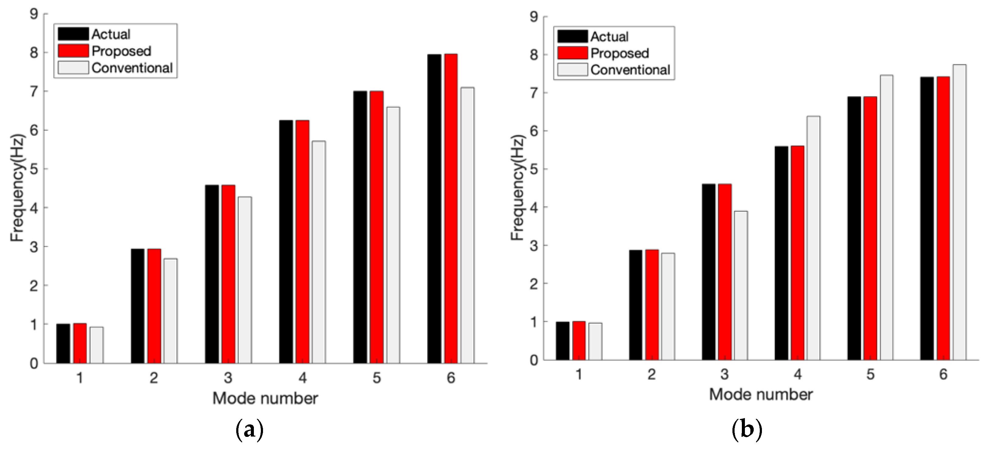
The updated frequencies by the proposed BMUA have a highly acceptable agreement and the error is less than 2% (herein, $\mathrm{error}=\left|f_{updated}-f_{actual}\right|/f_{actual}$, $f_{updated}$ and $f_{actual}$ are the updated frequency and the actual frequency, respectively), with actual values in two damage cases, as shown in

Table 4. Frequencies’ (Hz) comparison by the proposed and traditional approach.

	Damage No. 1			Damage No. 2
		Proposed Approach	Traditional Approach		Proposed Approach	Traditional Approach
Mode	Actual	Updated	Updated	Actual	Updated	Updated
1	1.0036	1.0182	0.9288	0.9944	1.0006	0.9672
2	2.9411	2.9379	2.6810	2.8743	2.8803	2.7870
3	4.5735	4.5821	4.273	4.6106	4.6115	3.8994
4	6.2419	6.2414	5.7089	5.5866	5.6004	6.3832
5	6.9934	6.9941	6.5862	6.8969	6.8956	7.4558
6	7.9430	7.9511	7.0902	7.4084	7.4125	7.7363

and Figure 4. In contrast, significant discrepancies between frequencies updated by the traditional BMUA and actual ones are observed: in damage case No. 1, 10.74% bias at the 6th frequency; in damage case No. 2, 14.26% bias at the 4th frequency. On the other hand, an excellent coincidence between the actual mode shapes and the proposed approach’s identified mode shapes is exhibited in Figure 5; nevertheless, the mode shapes acquired by traditional Bayesian greatly differ from the actual mode shapes.

Table 5. Results of updated structural parameters for damage case No.1.

		Proposed Approach			Traditional Approach
Parameter	Actual	Updated	S.D.	Error (%)	Updated	S.D.	Error (%)
${\mathsf{\beta }}_1$	1	1.0002	0.0032	0.02	1.0883	0.0018	8.83
${\mathsf{\beta }}_2$	1	0.9999	0.0019	0.01	0.87	0.0016	13.00
${\mathsf{\beta }}_3$	1	1.0001	0.0017	0.01	1.19	0.0014	19.00
${\mathsf{\beta }}_4$	1	0.9999	0.0019	0.01	0.7992	0.0012	20.08
${\mathsf{\beta }}_5$	0.8	0.7984	0.0018	0.20	1.1057	0.0089	38.21
${\mathsf{\beta }}_6$	1	0.9999	0.0009	0.01	0.9786	0.0043	2.14
${\mathsf{\theta }}_1$	0.9	0.8962	0.0019	0.42	0.83	0.0015	7.78
${\mathsf{\theta }}_2$	1	1.0014	0.0013	0.14	0.8654	0.0006	13.46
${\mathsf{\theta }}_3$	0.8	0.8014	0.0002	0.17	0.8165	0.0015	2.06
${\mathsf{\theta }}_4$	1	1.0013	0.0009	0.13	0.8191	0.0026	18.09
${\mathsf{\theta }}_5$	1	1.0014	0.0022	0.14	0.8209	0.0016	17.91
${\mathsf{\theta }}_6$	1	1.0014	0.0022	0.14	0.8063	0.0015	19.37

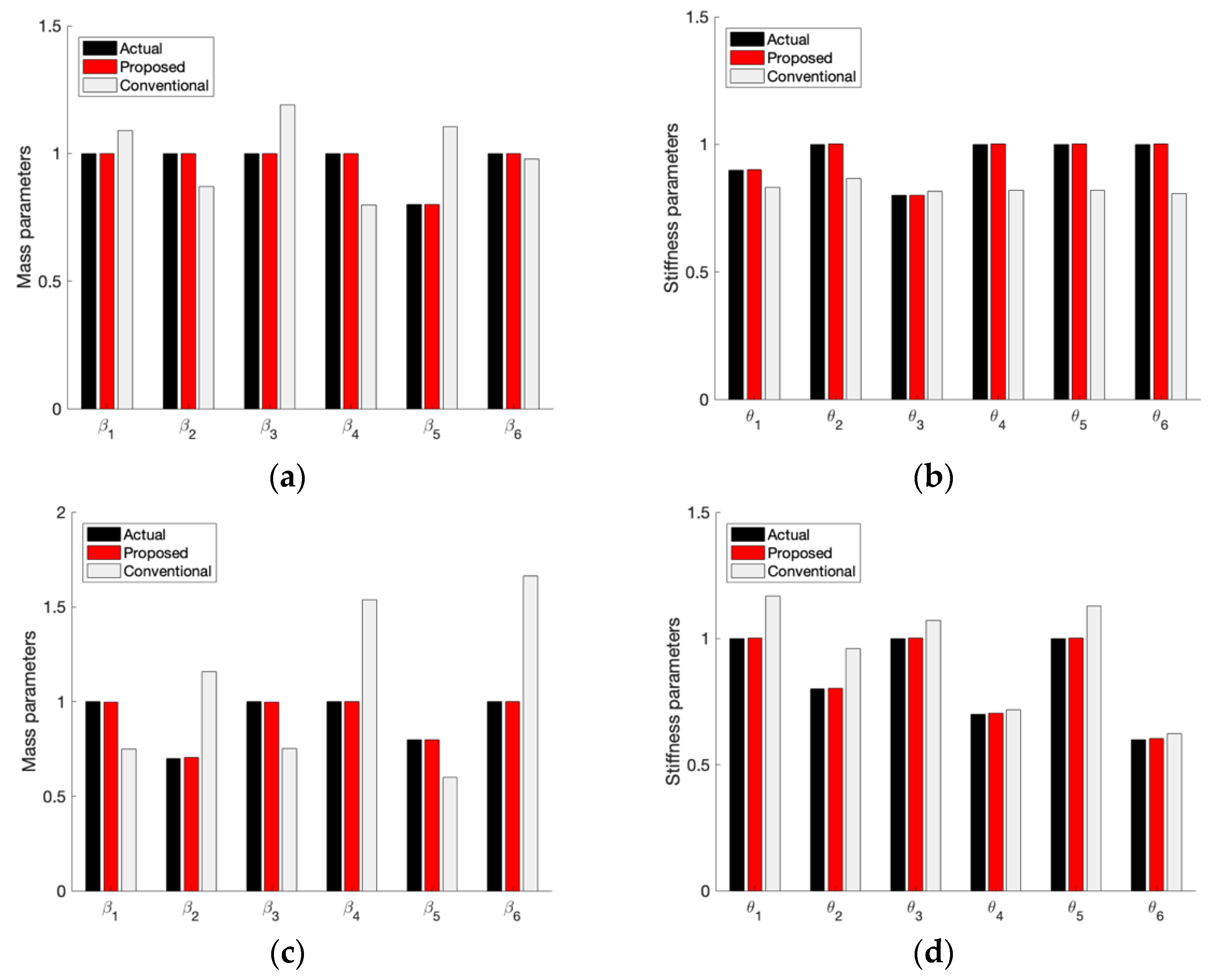
Note: $\mathsf{\beta }$ and $\mathsf{\theta }$ are mass and stiffness parameters, respectively; S.D. is standard derivation.

and

Table 6. Results of updated structural parameters for damage case No.2.

		Proposed Approach			Traditional Approach
Parameter	Actual	Updated	S.D.	Error (%)	Updated	S.D.	Error (%)
${\mathsf{\beta }}_1$	1	0.9965	0.0061	0.35	0.7477	0.003	25.23
${\mathsf{\beta }}_2$	0.7	0.6991	0.0105	0.13	1.1584	0.0028	65.49
${\mathsf{\beta }}_3$	1	0.9969	0.0085	0.31	0.752	0.0026	24.80
${\mathsf{\beta }}_4$	1	1.001	0.0055	0.10	1.5364	0.0024	53.64
${\mathsf{\beta }}_5$	0.8	0.7955	0.0024	0.56	0.6007	0.0019	24.91
${\mathsf{\beta }}_6$	1	0.9998	0.0006	0.02	1.6619	0.0019	66.19
${\mathsf{\theta }}_1$	1	1.0028	0.0025	0.28	1.1674	0.0049	16.74
${\mathsf{\theta }}_2$	0.8	0.7958	0.0012	0.53	0.9595	0.0024	19.94
${\mathsf{\theta }}_3$	1	1.0009	0.0012	0.09	1.0721	0.0028	7.21
${\mathsf{\theta }}_4$	0.7	0.7012	0.0011	0.17	0.7179	0.0032	2.56
${\mathsf{\theta }}_5$	1	1.0022	0.0008	0.22	1.1287	0.0013	12.87
${\mathsf{\theta }}_6$	0.6	0.5979	0.0007	0.35	0.623	0.0002	3.83

Note: $\mathsf{\beta }$ and $\mathsf{\theta }$ are mass and stiffness parameters, respectively; S.D. is standard derivation.

and Figure 6 present updated mass and stiffness parameters and corresponding uncertainties obtained from the proposed and the traditional BMUA in two damage cases. It is seen that the identified reduction in mass and stiffness parameters is almost identical to the actual values in terms of all damage cases by the proposed BMUA, indicating that the proposed BMUA is capable of outstanding performance on damage detection. However, actual and identified values using the traditional BMUA have a significant difference, e.g., the maximum error is 38% and 66% for both damage cases, respectively (see bold italic values in Table 5 and Table 6). It can be concluded that the traditional BMUA cannot detect damage induced by both reductions in mass and stiffness. This is attributable to the required assumption in the traditional BMUA that at least one between mass and stiffness has to be known and unchanged due to damage to avoid the coupling effect of mass and stiffness. This example also illustrates that a variation in mass or stiffness reflects that the damage extent cannot be ignored; if not, significant bias on updating results can mislead engineers’ judgment. In the proposed BMUA, the coupling effect of mass and stiffness is intrinsically addressed by employing two groups of data acquired from two systems—original and stiffness-modified system. As a result, a successful updating of mass and stiffness is achieved. In summary, the example of a six-story shear building demonstrates the proposed BMUA is superior to the traditional BMUA in simultaneously identifying mass and stiffness.

3.1.3. Probability of Damage Detection

The probability of damage is calculated based on the MPVs of mass and stiffness and corresponding the value of S.D. using Equation (54). It is found, in Figure 7, that the curves at the damaged location are distinguishable from those at a healthy location by observing the curve’s distance from healthy cases. Furthermore, some quantities can be interpreted from curves.

For damage case No. 1, the probabilistic curves of the mass parameter at the fifth floor (${\beta }_5$) and stiffness parameter $({\theta }_3$) at the third-floor exhibit high probabilities (77.88% and 80.66%, respectively) of both having a possible reduction of 20%. Regarding damage case No. 2, the mass on the second floor (${\beta }_2$) and stiffness on the fourth floor (${\theta }_4$) have a possible reduction of 30% with a high probability of 70.72% and 73.1%, respectively. The proposed BMUA exhibits excellent performance for damage detection; both localization and quantification of damages are successfully identified.

3.2. Three-Dimensional Three-Story Shear Building

A three-dimensional three-story shear building is utilized to evaluate the proposed BMUA under more complex conditions, including damage detection and comparative investigation between the traditional and the proposed BMUA in Section 3.2.1. Finally, probabilistic damage estimation is provided to predict structural failure in Section 3.2.2.

The diagram of the structural model is shown in Figure 8. In this example, the Young’s modulus and mass density are assumed to be 69 GPa and 2700 kg/m³, respectively. Each floor has the length and width of both 4.3 m with 0.2 m thickness, giving the mass weight of M = ${10}^4$ kg. Hence, a total of three mass parameters are to be updated. Four stiffness values at each floor are assumed, giving twelve to-be-updated stiffness parameters as ${\theta }_{4\left(j-1\right)+1}=K_{j,+x}$, ${\theta }_{4\left(j-1\right)+2}=K_{j,+y}$, ${\theta }_{4\left(j-1\right)+3}=K_{j,-x}$, ${\theta }_{4\left(j-1\right)+4}=K_{j,-y}$, $j=1,2,3$, where $j$ denotes the story number and $+x$, $-x$, $+y$ and $-y$ are the directions of the structural outer face. All columns have the same material and geometric properties with the length and moment of inertial of 5 m, 0.006 m⁴ ($y$-direction) and 0.0075 m⁴ ($x$-direction), respectively. The nominal magnitudes of inter-story stiffness are estimated to be $K_{j,+y}=K_{j,-y}=\mathrm{40,000} \mathrm{kN}/\mathrm{m}$ and $K_{j,+x}=K_{j,-x}=\mathrm{50,000} \mathrm{kN}/\mathrm{m}$.

An earthquake-damaged structure is repaired using a typical retrofitting technique. Let us suppose that the frame model is subject to unknown seismic activities, yielding severe structural damage, such as cracks and bearing deterioration, further impairing stiffness and ductility. Therefore, it is essential to repair the structure and strengthen its resistance capability to avoid any collapse. Herein, the Buckling-restrained brace (BRB) (see Figure 1c) is a useful seismic retrofit method and can provide additional stiffness and energy dissipation capacity [46]. In this work, twelve BRBs marked as red color are welded on the structure in four directions, as shown in Figure 8b. Assuming each BRB installed in the $x$- or $y$-direction has the same sectional and material properties (length of 6.59 m, moment of inertial of 0.0006 m⁴ ($x$-direction) and 0.0005 m⁴ ($y$-direction)), to provide the same stiffness modification, $∆k_{j,+x}=∆k_{j,-x}=1750 \mathrm{kN}/\mathrm{m}$, $∆k_{j,+y}=∆k_{j,-y}=1400 \mathrm{kN}/\mathrm{m}$ on each floor, the weight of each BRB is ignored here. In this example, the measured data contain the first six frequencies and mode shapes in the original and modified system with stiffness modification. Gaussian white noise with zero-mean and 1% COV of modal parameters is considered on the measured data for both the proposed BMUA and the traditional BMUA.

3.2.1. Damage Detection by the Proposed BMUA

Alterations in mass and stiffness parameters are used to mimic damage cases (see

Table 7. Damage cases.

Case No.	Mass Change	Stiffness Change
1	−20% (1st floor)	−15% (2nd floor, $+x$ face) −25% (3rd floor, $+y$ face)
2	−20% (2nd floor) −30% (3rd floor)	−20% (1st floor, $+x$ face) −30% (2nd floor, $-x$ face) −40% (3rd floor, $+\mathrm{y}$ face)

). The unity is defined as the initial value for each mass and stiffness parameter when detecting damage. A comparative investigation is also carried out to compare the proposed BMUA with the traditional counterpart. It is worth mentioning that, herein, the proposed and traditional BMUA adopt different eigenequations to update mass and stiffness; the former eliminates the coupling effect by Equations (11) and (17), but the latter still maintains the coupling effect in Equation (1).

Table 8. Frequencies’ (Hz) comparison by the proposed and traditional approach.

	Damage No. 1			Damage No. 2
		Proposed Approach	Traditional Approach		Proposed Approach	Traditional Approach
Mode	Actual	Updated	Updated	Actual	Updated	Updated
1	6.3474	6.3474	5.8556	7.1355	7.1546	6.3653
2	7.0487	7.0487	6.4986	7.5861	7.5070	6.6389
3	11.6205	11.6205	13.4559	12.7083	12.7832	13.2181
4	17.8686	17.8686	18.8641	17.8885	17.8452	20.0733
5	20.9130	20.9130	22.6068	20.4540	20.4990	23.3488
6	26.4592	26.4592	28.2637	26.5736	26.5364	29.6830

and Figure 9 present updated frequencies by the proposed and traditional BMUA in two damage cases. Frequencies are updated with a considerably accurate level using the proposed approach for all damage cases. However, frequencies are updated by the traditional approach with significant errors.

Table 9. MAC values by two approaches.

	Damage No. 1		Damage No. 2
Mode Number	Proposed Approach	Traditional Approach	Proposed Approach	Traditional Approach
1	0.9999	0.9974	1.0000	0.9989
2	1.0000	0.9994	1.0000	0.9968
3	0.9999	0.9988	1.0000	0.9984
4	1.0000	0.9987	1.0000	0.9891
5	0.9992	0.9994	1.0000	0.9962
6	0.9981	0.9945	0.9999	0.9955

lists diagonal values of the modal assurance criterion (MAC) for mode shapes by the proposed and traditional BMUA in terms of different damage cases. It is observed that the proposed approach’s mode shapes are consistent with the actual ones, while the traditional Bayesian approach provides biased MAC values. For example, the traditional approach yields an MAC value of 0.9891 at the fourth mode for the damage case No. 2; the proposed approach obtains an MAC value of 1.0000.

The MPVs and associated standard derivation (S.D.) by the two Bayesian approaches are shown in

Table 10. Results of updated structural parameters for damage case No. 1.

		Proposed Approach			Traditional Approach
Parameter	Actual	Updated	S.D.	Error (%)	Updated	S.D.	Error (%)
${\mathsf{\beta }}_1$	0.8	0.8003	0.0014	0.04	0.0109	0.0005	98.64
${\mathsf{\beta }}_2$	1	1.0008	0.0029	0.08	0.0865	0.001	91.35
${\mathsf{\beta }}_3$	1	0.9997	0.0015	0.03	0.0115	0.0008	98.85
${\mathsf{\theta }}_{1,+\mathrm{x}}$	1	0.9861	0.002	1.39	1.2308	0.0065	23.08
${\mathsf{\theta }}_{1,+\mathrm{y}}$	1	0.9943	0.0035	0.57	1.3491	0.0024	34.91
${\mathsf{\theta }}_{1,-\mathrm{x}}$	1	0.9833	0.0019	1.67	1.2325	0.0055	23.25
${\mathsf{\theta }}_{1,-\mathrm{y}}$	1	1.0052	0.0036	0.52	1.3921	0.0033	39.21
${\mathsf{\theta }}_{2,+\mathrm{x}}$	0.85	0.8485	0.0022	0.18	0.9335	0.0058	9.82
${\mathsf{\theta }}_{2,+\mathrm{y}}$	1	1.0046	0.0035	0.46	1.0801	0.004	8.01
${\mathsf{\theta }}_{2,-\mathrm{x}}$	1	1.0014	0.0027	0.14	1.1209	0.0063	12.09
${\mathsf{\theta }}_{2,-\mathrm{y}}$	1	0.9952	0.0039	0.48	1.072	0.005	7.20
${\mathsf{\theta }}_{3,+\mathrm{x}}$	1	1.0054	0.0041	0.54	1.0005	0.0037	0.05
${\mathsf{\theta }}_{3,+\mathrm{y}}$	0.75	0.7481	0.0011	0.25	0.728	0.0005	2.93
${\mathsf{\theta }}_{3,-\mathrm{x}}$	1	1.0102	0.0039	1.02	0.9943	0.0028	0.57
${\mathsf{\theta }}_{3,-\mathrm{y}}$	1	0.9994	0.0014	0.06	0.9804	0.0021	1.96

Note: $\mathsf{\beta }$ and $\mathsf{\theta }$ are mass and stiffness parameters, respectively; S.D. is standard derivation.

and

Table 11. Results of updated structural parameters for damage case No. 2.

		Proposed Approach			Traditional Approach
Parameter	Actual	Updated	S.D.	Error (%)	Updated	S.D.	Error (%)
${\mathsf{\beta }}_1$	1	0.9997	0.0025	0.03	0.0121	0.0141	98.79
${\mathsf{\beta }}_2$	0.8	0.8001	0.0009	0.01	0.0419	0.0033	94.76
${\mathsf{\beta }}_3$	0.7	0.6974	0.0051	0.37	0.0078	0.0007	98.89
${\mathsf{\theta }}_{1,+\mathrm{x}}$	0.8	0.7961	0.0036	0.49	0.6661	0.0014	16.74
${\mathsf{\theta }}_{1,+\mathrm{y}}$	1	1.0017	0.0035	0.17	0.9716	0.0034	2.84
${\mathsf{\theta }}_{1,-\mathrm{x}}$	1	0.9986	0.0041	0.14	0.8908	0.0031	10.92
${\mathsf{\theta }}_{1,-\mathrm{y}}$	1	0.9978	0.0039	0.22	0.934	0.0044	6.60
${\mathsf{\theta }}_{2,+\mathrm{x}}$	1	0.9938	0.0048	0.62	1.2327	0.0038	23.27
${\mathsf{\theta }}_{2,+\mathrm{y}}$	1	1.0265	0.0041	2.65	1.0861	0.0028	8.61
${\mathsf{\theta }}_{2,-\mathrm{x}}$	0.7	0.6956	0.0048	0.63	0.8386	0.0062	19.80
${\mathsf{\theta }}_{2,-\mathrm{y}}$	1	0.9727	0.0042	2.73	1.0948	0.0029	9.48
${\mathsf{\theta }}_{3,+\mathrm{x}}$	1	1.0194	0.0039	1.94	1.3141	0.0032	31.41
${\mathsf{\theta }}_{3,+\mathrm{y}}$	0.6	0.5986	0.003	0.23	0.8374	0.0019	39.57
${\mathsf{\theta }}_{3,-\mathrm{x}}$	1	0.9771	0.0046	2.29	1.3245	0.0016	32.45
${\mathsf{\theta }}_{3,-\mathrm{y}}$	1	0.9987	0.0048	0.13	1.3603	0.0018	36.03

Note: $\mathsf{\beta }$ and $\mathsf{\theta }$ are mass and stiffness parameters, respectively; S.D. is standard derivation.

. The proposed approach achieves satisfactory updating of mass and stiffness parameters. In contrast, the traditional Bayesian approach poorly updates mass and stiffness parameters. For example, it was found that, for damage case No. 1 in Table 10, the mass parameter ${\beta }_1$ and the stiffness parameter ${\theta }_{1,-y}$, are updated as 0.0109 and 1.3921 (target: 0.8000 and 1.0000), respectively; for damage case No. 2 in Table 11, the mass parameter and the stiffness parameter, ${\beta }_3$ and ${\theta }_{3,-y}$, are updated as 0.0078 and 1.3603 (target: 0.7000 and 1.0000).

As seen in Figure 10, the mass/stiffness parameters identified by the proposed approach highly agree with the target values for the considered damage cases. Only an error of less than 3% can be observed. However, mass/stiffness parameters are updated with prominent discrepancies by the traditional Bayesian approach; even some updated results are completely unacceptable, such as too-small values in the updated mass parameters. Similar to the first example, the traditional Bayesian approach fails to update both mass and stiffness parameters using the classical eigenequation in Equation (1), resulting in poor or false damage detection. It can be attributed to the coupling effect of mass and stiffness existing in traditional Bayesian that governs the accuracy of the updated results when simultaneously updating mass and stiffness.

3.2.2. Probability of Damage Detection

The MPVs of mass and stiffness under the damaged condition and corresponding uncertainties are utilized to compute the probability given a certain damage level. Figure 11 illustrates that, for damage case No.1, the mass parameter ${\beta }_1$ and the stiffness parameter ${\theta }_{3,+y}$ have a high probability (61.22% and 85.62%, respectively) of having possible damage—20% and 25%. For damage case No. 2, the mass parameter ${\beta }_2$ and the stiffness parameter ${\theta }_{3,+y}$ have a possible reduction of 20% and 40% with a high probability of 83.62% and 76.38%, respectively.

In practice, damage can be detected by probabilistic curves, because the curves related to damage locations are generally easily distinguished from the ones related to healthy locations. For example, the curves of ${\beta }_1$, ${\theta }_{2,+x}$ and ${\theta }_{3,+y}$ in damage case No.1 are clearly separated from the others, indicating that the location corresponding to ${\beta }_1$, ${\theta }_{2,+x}$ and ${\theta }_{3,+y}$ may have certain damage. A similar observation is found in damage case No. 2. The proposed method can detect damage in mass and stiffness along with location and severity. Engineers can be informed that some repairing work may be necessary at a certain location.

3.2.3. Discussion on Practical Aspects

This section presents the practical aspects, such as the accuracy, computation costs and practical applications, of the proposed BMUA in the real world. The two numerical examples in this paper illustrate that the proposed BMUA with stiffness modification has an advantage against the traditional BMUA in identifying mass and stiffness. In the traditional BMUA, at least one of mass and stiffness is accurately known to avoid the coupling effect, but this assumption is quite questionable; the traditional Bayesian ignores variations in mass or stiffness induced by possible damage. In contrast, the new BMUA with stiffness modification does not involve any assumption on mass and stiffness properties. In short, the proposed BMUA enables to deal with the coupling effect of mass and stiffness in order to successfully identify mass and stiffness. However, the traditional BMUA poorly updates both mass and stiffness because of the coupling effect caused by the classical eigenequation in Equation (1).

Possible implementations in practice of the proposed BMUA with stiffness modification are described in Section 1 (see Figure 1). The magnitude of stiffness modification could be conveniently determined once the sectional properties of added structural components or the technical specification of the devices are known [65,66]. Regarding the computational cost, the proposed Bayesian updating approach exhibites high efficiency, because the analytical formulations of the model parameters and uncertainty quantification are explicitly derived. The model updating work by the proposed Bayesian approach was carried out on the laptop flatform of MacBook Pro 2017 with 3.1 GHz Dual-Core Intel Core i5 for the two numerical examples. The six- and twelve-dimensional problem in the first and second example only took around 4 s and 8 s, respectively, suggesting that the proposed approach is fast-running and practically valuable even for real-time model updating.

Let us remark that the number of data sets does not affect the performance of the proposed BMUA against the traditional BMUA. The proposed BMUA adopts new eigenequations in Section 2.4. Only two groups of measured data are used to remove the coupling effect. Although BMUA is significantly promising, the proposed approach’s performance under lab or field test conditions needs to be examined in future work.

4. Conclusions and Summary

The significance of the present work is to propose a new Bayesian model updating framework to identify both mass and stiffness as well as associated uncertainties without the coupling effect of mass and stiffness when the repair or retrofitting techniques are applied to damaged structures. This approach allows engineers to estimate the mass and stiffness before repair and retrofitting, leading to provide the full spectrum (pre-repair and post-repair conditions) using the application of retrofitting techniques. The practical application for stiffness modification can be convenient and accessible, such as repair and retrofitting strategies used to restore structural performance, which usually requires additional stiffness (described in Figure 1). The proposed approach can intrinsically address the coupling effect of mass and stiffness by stiffness modification and achieve accurate updating of mass and stiffness.

The comparative study also shows that the proposed BMUA is more accurate and reliable than the traditional one in updating both mass and stiffness. The probabilistic damage estimation in the critical structural parameters is also accomplished by the proposed approach to better predict the structural conditions and assess the structural reliability (probability of failure). In addition, the probabilistic curve allows engineers to intuitively localize damage and provides some preliminary insight into damage detection. Finally, a tangible and measurable quantity to estimate structural integrity can advance the existing post-disaster management.

Although the proposed Bayesian updating approach has potential in real applications for SHM, it still has some limitations that need to be addressed in future studies. For instance, the damping ratio exhibits more sensitivity to local damage, e.g., holes and cracks; hence, it should be integrated into objective functions to improve the capability of detecting damage for the current Bayesian model updating approach.

References

- Chen, H.-P. Structural Health Monitoring of Large Civil Engineering Structures; John Wiley & Sons: Hoboken, NJ, USA, 2018. [Google Scholar]
- Balageas, D.; Fritzen, C.-P.; Güemes, A. Structural Health Monitoring; John Wiley & Sons: Hoboken, NJ, USA, 2010; Volume 90. [Google Scholar]
- Singh, V.P.; Jain, S.K.; Tyagi, A. Risk and reliability analysis: A handbook for civil and environmental engineers. In Proceedings of the American Society of Civil Engineers, Pittsburgh, PA, USA, 24–27 July 2007. [Google Scholar]
- Jensen, H.A.; Vergara, C.; Papadimitriou, C.; Millas, E. The use of updated robust reliability measures in stochastic dynamical systems. Comput. Methods Appl. Mech. Eng. 2013, 267, 293–317. [Google Scholar] [CrossRef]
- Varadarajan, N.; Nagarajaiah, S. Wind response control of building with variable stiffness tuned mass damper using empirical mode decomposition/Hilbert transform. J. Eng. Mech. 2004, 130, 451–458. [Google Scholar] [CrossRef] [Green Version]
- Yang, J.N.; Agrawal, A.K.; Samali, B.; Wu, J.-C. Benchmark problem for response control of wind-excited tall buildings. J. Eng. Mech. 2004, 130, 437–446. [Google Scholar] [CrossRef]
- Mustafa, S.; Matsumoto, Y. Bayesian Model Updating and Its Limitations for Detecting Local Damage of an Existing Truss Bridge. J. Bridge Eng. 2017, 22, 04017019. [Google Scholar] [CrossRef]
- Mottershead, J.E.; Link, M.; Friswell, M.I. The sensitivity method in finite element model updating: A tutorial. Mech. Syst. Signal Process. 2011, 25, 2275–2296. [Google Scholar] [CrossRef]
- Wan, H.-P.; Ren, W.-X. Stochastic model updating utilizing Bayesian approach and Gaussian process model. Mech. Syst. Signal Process. 2016, 70–71, 245–268. [Google Scholar] [CrossRef]
- Marwala, T. Finite Element Model Updating Using Computational Intelligence Techniques: Applications to Structural Dynamics; Springer Science & Business Media: Berlin, Germany, 2010. [Google Scholar]
- Huang, M.; Cheng, X.; Zhu, Z.; Luo, J.; Gu, J. A Novel Two-Stage Structural Damage Identification Method Based on Superposition of Modal Flexibility Curvature and Whale Optimization Algorithm. Int. J. Struct. Stab. Dyn. 2021, 21, 2150169. [Google Scholar] [CrossRef]
- Huang, M.; Cheng, X.; Lei, Y. Structural damage identification based on substructure method and improved whale optimization algorithm. J. Civ. Struct. Health Monit. 2021, 11, 351–380. [Google Scholar] [CrossRef]
- Xu, Z.; Huang, M. Improving Bridge Expansion and Contraction Installation Replacement Decision System Using Hybrid Chaotic Whale Optimization Algorithm. Appl. Sci. 2021, 11, 6222. [Google Scholar] [CrossRef]
- Su, Y.; Liu, L.; Lei, Y. Structural Damage Identification Using a Modified Directional Bat Algorithm. Appl. Sci. 2021, 11, 6507. [Google Scholar] [CrossRef]
- He, M.; Sun, L.; Zeng, X.; Liu, W.; Tao, S. Node layout plans for urban underground logistics systems based on heuristic bat algorithm. Comput. Commun. 2020, 154, 465–480. [Google Scholar] [CrossRef]
- Wei, Z.; Liu, J.; Lu, Z. Structural damage detection using improved particle swarm optimization. Inverse Probl. Sci. Eng. 2018, 26, 792–810. [Google Scholar] [CrossRef]
- Vaez, S.R.H.; Fallah, N. Damage detection of thin plates using GA-PSO algorithm based on modal data. Arab. J. Sci. Eng. 2017, 42, 1251–1263. [Google Scholar] [CrossRef]
- Huang, M.; Li, X.; Lei, Y.; Gu, J. Structural damage identification based on modal frequency strain energy assurance criterion and flexibility using enhanced Moth-Flame optimization. Structures 2020, 28, 1119–1136. [Google Scholar] [CrossRef]
- Huang, M.; Lei, Y. Bearing damage detection of a reinforced concrete plate based on sensitivity analysis and chaotic moth-flame-invasive weed optimization. Sensors 2020, 20, 5488. [Google Scholar] [CrossRef] [PubMed]
- Huang, M.-S.; Gül, M.; Zhu, H.-P. Vibration-Based Structural Damage Identification under Varying Temperature Effects. J. Aerosp. Eng. 2018, 31, 04018014. [Google Scholar] [CrossRef]
- Alexandrino, P.d.S.L.; Gomes, G.F.; Cunha, S.S., Jr. A robust optimization for damage detection using multiobjective genetic algorithm, neural network and fuzzy decision making. Inverse Probl. Sci. Eng. 2020, 28, 21–46. [Google Scholar] [CrossRef]
- Beck, J.L.; Au, S.-K. Bayesian Updating of Structural Models and Reliability using Markov Chain Monte Carlo Simulation. J. Eng. Mech. 2002, 128, 380–391. [Google Scholar] [CrossRef]
- Mares, C.; Mottershead, J.; Friswell, M. Stochastic model updating: Part 1—Theory and simulated example. Mech. Syst. Signal Process. 2006, 20, 1674–1695. [Google Scholar] [CrossRef]
- Khodaparast, H.H.; Mottershead, J.E.; Friswell, M.I. Perturbation methods for the estimation of parameter variability in stochastic model updating. Mech. Syst. Signal Process. 2008, 22, 1751–1773. [Google Scholar] [CrossRef]
- Chatzi, E.N.; Smyth, A.W. The unscented Kalman filter and particle filter methods for nonlinear structural system identification with non-collocated heterogeneous sensing. Struct. Control Health Monit. 2009, 16, 99–123. [Google Scholar] [CrossRef]
- Moens, D.; Vandepitte, D. Interval sensitivity theory and its application to frequency response envelope analysis of uncertain structures. Comput. Methods Appl. Mech. Eng. 2007, 196, 2486–2496. [Google Scholar] [CrossRef]
- Lam, H.-F.; Hu, J.; Zhang, F.-L.; Ni, Y.-C. Markov chain Monte Carlo-based Bayesian model updating of a sailboat-shaped building using a parallel technique. Eng. Struct. 2019, 193, 12–27. [Google Scholar] [CrossRef]
- Hu, J.; Yang, J.-H. Operational Modal Analysis and Bayesian Model Updating of a Coupled Building. Int. J. Struct. Stab. Dyn. 2019, 19, 1940012. [Google Scholar] [CrossRef]
- Li, M.; Jia, G. Bayesian Updating of Bridge Condition Deterioration Models Using Complete and Incomplete Inspection Data. J. Bridge Eng. 2020, 25, 04020007. [Google Scholar] [CrossRef]
- Yang, J.; Lam, H.F.; Hu, J. Ambient Vibration Test, Modal Identification and Structural Model Updating Following Bayesian Framework. Int. J. Struct. Stab. Dyn. 2015, 15, 1540024. [Google Scholar] [CrossRef]
- Sedehi, O.; Papadimitriou, C.; Katafygiotis, L.S. Probabilistic hierarchical Bayesian framework for time-domain model updating and robust predictions. Mech. Syst. Signal Process. 2019, 123, 648–673. [Google Scholar] [CrossRef]
- Beck, J.L.; Katafygiotis, L.S. Updating models and their uncertainties. I: Bayesian statistical framework. J. Eng. Mech. 1998, 124, 455–461. [Google Scholar] [CrossRef]
- Katafygiotis, L.S.; Beck, J.L. Updating models and their uncertainties. II: Model identifiability. J. Eng. Mech. 1998, 124, 463–467. [Google Scholar] [CrossRef]
- Yuen, K.-V.; Beck, J.L.; Katafygiotis, L.S. Efficient model updating and health monitoring methodology using incomplete modal data without mode matching. Struct. Control. Health Monit. 2006, 13, 91–107. [Google Scholar] [CrossRef]
- Das, A.; Debnath, N. A Bayesian finite element model updating with combined normal and lognormal probability distributions using modal measurements. Appl. Math. Model. 2018, 61, 457–483. [Google Scholar] [CrossRef]
- Yan, W.-J.; Katafygiotis, L.S. A novel Bayesian approach for structural model updating utilizing statistical modal information from multiple setups. Struct. Saf. 2015, 52, 260–271. [Google Scholar] [CrossRef]
- Cheung, S.H.; Bansal, S. A new Gibbs sampling based algorithm for Bayesian model updating with incomplete complex modal data. Mech. Syst. Signal Process. 2017, 92, 156–172. [Google Scholar] [CrossRef]
- Xu, B.; Deng, B.-C.; Li, J.; He, J. Structural nonlinearity and mass identification with a nonparametric model using limited acceleration measurements. Adv. Struct. Eng. 2018, 22, 1018–1031. [Google Scholar] [CrossRef]
- Zhang, D.; Li, H. Loop substructure identification for shear structures of unknown structural mass using synthesized references. Smart Mater. Struct. 2017, 26, 085046. [Google Scholar] [CrossRef]
- Do, N.T.; Gül, M. Structural damage detection under multiple stiffness and mass changes using time series models and adaptive zero-phase component analysis. Struct. Control Health Monit. 2020, 27, e2577. [Google Scholar] [CrossRef]
- Lei, Y.; Qiu, H.; Zhang, F. Identification of structural element mass and stiffness changes using partial acceleration responses of chain-like systems under ambient excitations. J. Sound Vib. 2020, 488, 115678. [Google Scholar] [CrossRef]
- Ding, Z.; Zhao, Y.; Lu, Z. Simultaneous identification of structural stiffness and mass parameters based on Bare-bones Gaussian Tree Seeds Algorithm using time-domain data. Appl. Soft Comput. 2019, 83, 105602. [Google Scholar] [CrossRef]
- Fathizadeh, S.F.; Dehghani, S.; Yang, T.Y.; Vosoughi, A.R.; Noroozinejad Farsangi, E.; Hajirasouliha, I. Seismic performance assessment of multi-story steel frames with curved dampers and semi-rigid connections. J. Constr. Steel Res. 2021, 182, 106666. [Google Scholar] [CrossRef]
- Kazemi, F.; Mohebi, B.; Jankowski, R. Predicting the seismic collapse capacity of adjacent SMRFs retrofitted with fluid viscous dampers in pounding condition. Mech. Syst. Signal Process. 2021, 161, 107939. [Google Scholar] [CrossRef]
- Saingam, P.; Sutcu, F.; Terazawa, Y.; Fujishita, K.; Lin, P.-C.; Celik, O.C.; Takeuchi, T. Composite behavior in RC buildings retrofitted using buckling-restrained braces with elastic steel frames. Eng. Struct. 2020, 219, 110896. [Google Scholar] [CrossRef]
- FEMA—Federal Emergency Management Agency. Techniques for the Seismic Rehabilitation of Existing Buildings; FEMA: Hyattsville, MD, USA, 2006.
- Khatibi, M.M.; Ashory, M.R.; Malekjafarian, A.; Brincker, R. Mass–stiffness change method for scaling of operational mode shapes. Mech. Syst. Signal Process. 2012, 26, 34–59. [Google Scholar] [CrossRef]
- López-Aenlle, M.; Brincker, R.; Pelayo, F.; Canteli, A.F. On exact and approximated formulations for scaling-mode shapes in operational modal analysis by mass and stiffness change. J. Sound Vib. 2012, 331, 622–637. [Google Scholar] [CrossRef]
- Yao, Y.; Yan, M.; Shi, Z.; Wang, Y.; Bao, Y. Mechanical behavior of an innovative steel–concrete joint for long-span railway hybrid box girder cable-stayed bridges. Eng. Struct. 2021, 239, 112358. [Google Scholar] [CrossRef]
- Barbagallo, F.; Bosco, M.; Marino, E.M.; Rossi, P.P. Seismic design and performance of dual structures with BRBs and semi-rigid connections. J. Constr. Steel Res. 2019, 158, 306–316. [Google Scholar] [CrossRef]
- Liu, Y.; Zhang, Q.; Bao, Y.; Bu, Y. Static and fatigue push-out tests of short headed shear studs embedded in Engineered Cementitious Composites (ECC). Eng. Struct. 2019, 182, 29–38. [Google Scholar] [CrossRef]
- Vianna, J.d.C.; Costa-Neves, L.F.; Vellasco, P.D.S.; de Andrade, S.A.L. Experimental assessment of Perfobond and T-Perfobond shear connectors’ structural response. J. Constr. Steel Res. 2009, 65, 408–421. [Google Scholar] [CrossRef]
- Yuen, K.-V. Bayesian Methods for Structural Dynamics and Civil Engineering; John Wiley & Sons: Hoboken, NJ, USA, 2010. [Google Scholar]
- Coppotelli, G. On the estimate of the FRFs from operational data. Mech. Syst. Signal Process. 2009, 23, 288–299. [Google Scholar] [CrossRef]
- Au, S. Chapter 14: Multi-Setup Problem. Operational Modal Analysis: Modeling, Bayesian Inference, Uncertainty Laws; Springer: Singapore, 2017; p. 541. [Google Scholar]
- Zeng, J.; Kim, Y.H. Identification of Structural Stiffness and Mass using Bayesian Model Updating Approach with Known Added Mass: Numerical Investigation. Int. J. Struct. Stab. Dyn. 2020, 20, 2050123. [Google Scholar] [CrossRef]
- Hızal, Ç.; Turan, G. A two-stage Bayesian algorithm for finite element model updating by using ambient response data from multiple measurement setups. J. Sound Vib. 2020, 469, 115139. [Google Scholar] [CrossRef]
- Rezaiee-Pajand, M.; Entezami, A.; Sarmadi, H. A sensitivity-based finite element model updating based on unconstrained optimization problem and regularized solution methods. Struct. Control Health Monit. 2020, 27, e2481. [Google Scholar] [CrossRef]
- Chen, H.-P.; Tee, K.F.; Ni, Y.-Q. Mode shape expansion with consideration of analytical modelling errors and modal measurement uncertainty. Smart Struct. Syst. 2012, 10, 485–499. [Google Scholar] [CrossRef]
- Chen, H.-P. Mode shape expansion using perturbed force approach. J. Sound Vib. 2010, 329, 1177–1190. [Google Scholar] [CrossRef]
- Lam, H.F.; Yang, J.H.; Au, S.K. Markov chain Monte Carlo-based Bayesian method for structural model updating and damage detection. Struct. Control Health Monit. 2018, 25, e2140. [Google Scholar] [CrossRef]
- Au, S.-K.; Zhang, F.-L.; Ni, Y.-C. Bayesian operational modal analysis: Theory, computation, practice. Comput. Struct. 2013, 126, 3–14. [Google Scholar] [CrossRef]
- Au, S.-K. Fast Bayesian FFT method for ambient modal identification with separated modes. J. Eng. Mech. 2011, 137, 214–226. [Google Scholar] [CrossRef]
- Zeng, J.; Kim, Y.H. A two-stage framework for automated operational modal identification. Struct. Infrastruct. Eng. 2021, 1–20. [Google Scholar] [CrossRef]
- Ziemian, R.D.; Ziemian, C.W. Formulation and validation of minimum brace stiffness for systems of compression members. J. Constr. Steel Res. 2017, 129, 263–275. [Google Scholar] [CrossRef]
- D’Aniello, M.; Costanzo, S.; Landolfo, R. The influence of beam stiffness on seismic response of chevron concentric bracings. J. Constr. Steel Res. 2015, 112, 305–324. [Google Scholar] [CrossRef]
Figure 1.
Additional components for stiffness modification: (a) curved damper [44]; (b) fluid viscous damper [45]; (c) buckling-restrained brace [46]; (d) steel diagonal brace [43]; (e) springs [48].
Figure 2.
Six-story shear building: (a) original system; (b) modified system with curved dampers.
Figure 3.
Updated mode shapes using incomplete modes.
Figure 4.
Updated frequencies by two approaches: (a) damage case No. 1; (b) damage case No. 2.
Figure 5.
Updated mode shapes by two approaches: (a) damage case No. 1; (b) damage case No. 2.
Figure 6.
Updated parameters by two approaches. Damage case No. 1: (a) mass; (b) stiffness. Damage case No. 2: (c) mass; (d) stiffness.
Figure 7.
Probabilistic curves. Damage case No. 1: (a) mass; (b) stiffness. No. 2: (c) mass; (d) stiffness.
Figure 8.
Diagram of steel frame model: (a) original system and plan view; (b) modified system with BRBs (marked as red color).
Figure 9.
Figure 10.
Figure 11.