Vehicle State Estimation Using Interacting Multiple Model Based on Square Root Cubature Kalman Filter

Abstract

The distributed drive arrangement form has better potential for cooperative control of dynamics, but this drive arrangement form increases the parameter acquisition workload of the control system and increases the difficulty of vehicle control accordingly. In order to observe the vehicle motion state accurately and in real-time, while reducing the effect of uncertainty in noise statistical information, the vehicle state observer is designed based on interacting multiple model theory with square root cubature Kalman filter (IMM-SCKF). The IMM-SCKF algorithm sub-model considers different state noise and measurement noise, and the introduction of the square root filter reduces the complexity of the algorithm while ensuring accuracy and real-time performance. To estimate the vehicle longitudinal, lateral, and yaw motion states, the algorithm uses a three degree of freedom (3-DOF) vehicle dynamics model and a nonlinear brush tire model, which is then validated in a Carsim-Simulink co-simulation platform for multiple operating conditions. The results show that the IMM-SCKF algorithm’s fusion output results can effectively follow the sub-model with smaller output errors, and that the IMM-SCKF algorithm’s results are superior to the traditional SCKF algorithm’s results.

1. Introduction

Artificial intelligence technology has been promoted and applied to a variety of fields in recent years, and vehicles are moving closer to intelligence and electrification, with more advanced active safety control systems and intelligent driver assistance systems being installed in vehicles. A large amount of vehicle dynamics information, such as yaw rate, sideslip angle, lateral velocity, and longitudinal velocity, is used in the development of related control systems. The acquisition of this data in real time necessitates the use of high-accuracy sensors, which are costly and prone to issues such as sensor errors and uncertainties. Furthermore, unreliable measurement data can cause dispersion in the vehicle controller, which can have serious consequences. Therefore, state estimation methods for measurement information based on low-cost sensors have been widely tried and applied to vehicles [1]. Distributed-drive electric vehicles drive directly with in-wheel motors, replacing mechanical transmission and hydraulic systems with wire control systems, greatly simplifying the vehicle chassis structure and increasing mechanical efficiency. For distributed drive electric vehicles, a large number of control studies have been conducted. Electronic body stability systems, such as yaw moment control, use the quick response of four-wheel motors to improve the vehicle control system’s performance. Distributed-drive electric vehicles’ steering, driving, and braking signals are more accessible than those of conventional vehicles, effectively improving the vehicle’s sensing capability and making real-time observation of vehicle dynamics parameters easier [2]. Accurate vehicle state estimation results directly improve the sensing capability of intelligence vehicles, which is important for path tracking, trajectory tracking, and active safety controller design of intelligence vehicles. Mohamed Fnadi et al. proposed a nonlinear tire stiffness observer for the real-time tire stiffness estimation problem, and the Kalman-Bucy filter was used for lateral velocity estimation and a constrained MPC path tracking controller based on accurate state parameter information was proposed to improve the effectiveness of path tracking [3,4]. Hyo-Seok Kang et al. designed a robust tracking control method based on the estimation results provided by the state observer [5]. Song Yitong et al. designed a chassis controller integrated with four-wheel independent steering system and a direct yaw moment control system integrated with MPC based on the vehicle state estimation results provided by the UKF observer, which fully improved the stability of the vehicle [6].

A large number of studies based on kinematic and vehicle dynamics models have been conducted on vehicle state estimation. Tire-road conditions and vehicle parameters have no effect on kinematic-based state estimation, but the integration of sensor measurements generates cumulative errors that lead to large deviations in the results, so the method is only applicable to steady-state situations. The state estimation based on the dynamics model is also divided into two categories. The first is the linear two-degree-of-freedom (2-DOF) vehicle model, which is derived from the linear tire model and has a high estimation accuracy in conditions with small tire slip angle and is widely used to estimate the yaw rate and sideslip angle [7,8]. However, when the vehicle is operating in extreme conditions, the steering angle is large, the tire slip angle increases, and the tire enters the nonlinear region, the linear tire model does not accurately reflect the real vehicle dynamics. As a result of the large difference between the estimated and real values, the vehicle controller receives the result and makes an incorrect decision, resulting in serious consequences. In extreme operating conditions, the estimation method based on the nonlinear vehicle dynamics model has a high estimation accuracy [9]. Wang Zhenfeng et al., based on the Takagi-Sugeno (T-S) fuzzy model to describe the lateral force of tires, design a T-S fuzzy observer to estimate the vehicle roll state, and use the linear matrix inequalities (LMIs) criterion to prove the observer’s stability to solve the nonlinear problem of lateral force of vehicle under large lateral deflection angle working condition [10]. To solve the problem of inertial parameter changes such as the center of gravity position when the vehicle load changes, Dasol Jeong et al., proposed an algorithm based on smart tires combined with a nonlinear vehicle dynamics model to estimate tire loads and vehicle parameters, which has a higher sampling rate and better robustness in estimating tire loads [11]. Henning et al. proposed an integrated control method for lateral dynamics, combining nonlinear vehicle state and parameter estimation with a second-order differential Kalman filter to build a nonlinear vehicle model capable of accurately estimating the peak pavement adhesion coefficient as well as the sideslip angle under extreme operating conditions [12].

In recent years, more nonlinear estimation algorithms have been used in the field of vehicles. Among them are various Kalman filter derivative algorithms, such as extended Kalman filter (EKF), unscented Kalman filter (UKF), and cubature Kalman filter (CKF). When the vehicle model is complex, the EKF algorithm has trouble solving complex Jacobian matrices, while the UKF algorithm has high computational complexity. CKF is a Gaussian weighted integral approximation algorithm based on the third-order spherical-phase diameter volume rule proposed by Canadian scholars Arasaratnam and Haykin in recent years. The square root cubature Kalman filter (SCKF) is an improved algorithm based on the CKF that uses square root approximation recursion to effectively reduce the algorithm’s computational complexity while ensuring accuracy, stability, and real-time performance [13,14]. To design the vehicle state observer, which is based on the Kalman filter algorithm, it is essential to have a more accurate mathematical model as well as statistical properties of the known noise; otherwise, the prediction results will have large errors and even divergence in severe cases [15]. Zhang Zhida et al., used a weighted adaptive sliding window algorithm to adaptively adjust the measurement and process noise matrices of the SCKF algorithm, which has more improved accuracy and robustness than the conventional method [16]. Cheng Shuo et al. used an adaptive fusion of the estimated and integrated values to accurately estimate the vehicle sideslip angle by considering the sensor’s unknown color noise and correcting the integration term [17]. Most literature addressing the problem of statistical noise uncertainty employs adaptive corrections to measure and process noise in order to make accurate predictions.

The interacting multiple model Kalman filter method has been widely used in the field of target tracking and extended to many fields such as vehicle state estimation [18,19]. Liu HQ et al. based work on the framework of an interacting multiple model approach to update the probability of target state estimation and motion model by distance-rate measurement. Combined with SCKF algorithm to cope with the nonlinearity of the measurement equation, the designed IMM-SCKF algorithm has good performance in maneuvering target tracking [20]. Rui Song et al. designed SCKF with different error covariance matrices based on an interacting multiple model framework in order to solve the uncertainty of the error covariance of the navigation system in vehicle dynamics state estimation, and the results show that the IMM-SCKF algorithm has better accuracy compared with the traditional method [21]. In order to adapt to different vehicle-road system models, X Jin et al. designed a vehicle side slip angle state estimator based on interacting multiple model unscented Kalman filter (IMM-UKF) and analyzed the applicability of the nonlinear tire model under large tire side slip angle operating conditions [22]. In previous research work, interacting multiple model methods are often combined with nonlinear Kalman filter and have shown good performance in areas such as target tracking, navigation, etc., but there have been no applications to extend the IMM-SCKF algorithm to the field of vehicle state estimation.

Therefore, this paper proposes an interacting multiple model algorithm combined with square root cubature Kalman filter to design interacting multiple model sets based on nonlinear vehicle dynamics models for the case where the statistical characteristics of system state noise and measurement noise are unknown. The SCKF algorithm is used to estimate the yaw rate, sideslip angle, and longitudinal and lateral vehicle speeds for each sub-model, ensuring that the fusion estimation results always maintain the output of the sub-model with the least tracking error.

2. Vehicle and Tire Model

In this section, the vehicle dynamics model and tire model for vehicle state estimation are proposed to describe the vehicle motion state.

2.1. Vehicle Model

An overly complex vehicle model is not conducive to the real-time performance of the algorithm, so this paper establishes a three-degree-of-freedom (3-DOF) nonlinear vehicle dynamics model under the premise of satisfying the observation accuracy of vehicle dynamics and makes the following assumptions [23].

(1)

Assume that the pitch, vertical, and roll motion of the vehicle are ignored, and the influence of the suspension is ignored.

(2)

Ignore the influence of the camber angle and self-aligning torque of the wheels on the vehicle dynamics performance.

According to D’Alembert’s principle, a 3-DOF vehicle dynamics model containing yaw, longitudinal, and lateral motions was established, as shown in Figure 1, and the entire vehicle dynamics equations were established as follows:

Longitudinal motion:

$${\dot{V}}_x={\displaystyle \sum _{i,j=1}^2{F}_{xij}}/m+V_y\dot{\psi }$$

(1)

$${\displaystyle \sum _{i,j=1}^2{F}_{xij}}=F_{x11}\cos {\delta }_{11}+F_{x12}\cos {\delta }_{12}-F_{y11}\sin {\delta }_{11}-F_{y12}\sin {\delta }_{12}+F_{x21}+F_{x22}$$

(2)

Lateral motion:

$${\dot{V}}_y={\displaystyle \sum _{i,j=1}^2{F}_{yij}}/m+V_x\dot{\psi }$$

(3)

$${\displaystyle \sum _{i,j=1}^2{F}_{yij}}=F_{x11}\sin {\delta }_{11}+F_{x12}\sin {\delta }_{12}+F_{y11}\cos {\delta }_{11}+F_{y12}\cos {\delta }_{12}+F_{y21}+F_{y22}$$

(4)

Yaw motion:

$$\ddot{\psi }={\displaystyle \sum _{i,j=1}^2{M}_z{}_{ij}}/I_{zz}$$

(5)

$$\begin{array}{r}{\displaystyle \sum _{i,j=1}^2{M}_z{}_{ij}}=a(F_{y11}\cos {\delta }_{11}+F_{y12}\cos {\delta }_{12})+a(F_{x11}\sin {\delta }_{11}+F_{x12}\sin {\delta }_{12})-\frac{w}{2}(F_{y11}\sin {\delta }_{11}-F_{y12}\sin {\delta }_{12})+\\ \frac{w}{2}(F_{x11}\cos {\delta }_{11}-F_{x12}\cos {\delta }_{12})-(L-a)(F_{y21}+F_{y22})+\frac{w}{2}(F_{x21}-F_{x22})\end{array}$$

(6)

where $V_x$ is the vehicle longitudinal velocity, $V_y$ is the lateral velocity, $\dot{\psi }$ is the yaw rate, $a_x$ is the longitudinal acceleration, $a_y$ is the lateral acceleration, $M_z$ is the yaw moment, $F_{xij}$ and $F_{yij}$ are longitudinal and lateral forces of the tire (ij is 11, 12, 21, and 22, which represent the front left, front right, rear left, and rear right wheel, respectively), m is the vehicle mass, a is the distance from the center of mass to the front axle, b is the distance from rear axle to the center of gravity, w is the wheel track, L is the wheelbase, $I_{zz}$ is the yaw moment of inertia, and ${\delta }_{11}$ and ${\delta }_{12}$ are the steering angles of the left and right front wheels, respectively.

2.2. Brush Tire Model

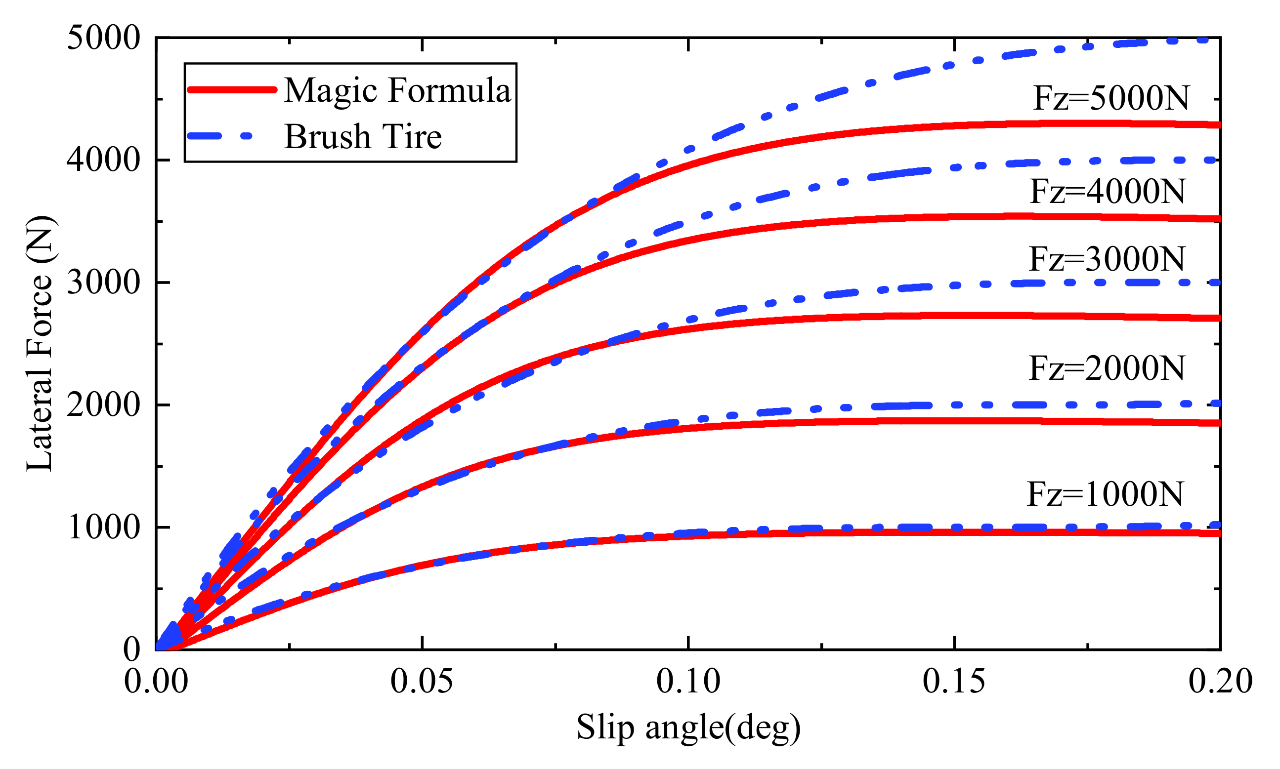
According to the above formula, the calculation of vehicle state requires known longitudinal and lateral tire forces, which are generally calculated using a tire model in vehicle dynamics research, and the accuracy of the tire model directly affects the accuracy of state estimation. Compared with the currently widely used Magic Formula (MF) tire model, the brush tire model requires fewer parameters to be fitted and can accurately represent the longitudinal and lateral forces of the tire, so the brush tire model is used for simulation in this paper [24].

As can be seen in Figure 2, the brush tire model has a high fitting accuracy under the small lateral deflection angle condition, but the peak lateral force of the brush tire model is slightly larger than that of the MF tire model under the large slip angle condition. In this paper, the simulation conditions are low vertical force and lateral slip angle, and the tires are not in the strong nonlinear region, so the brush tire model is chosen to ensure the simulation accuracy. The brush tire model calculation is shown below.

The joint longitudinal force and lateral force model is defined as:

$$\begin{gathered} f=\left\{\begin{array}{lll}\rho s& -\frac{{(\rho s)}^2}{3\mu F_z}+\frac{{(\rho s)}^3}{27{(\mu F_z)}^2}& \left|s\right|<s_m\\ \mu F_z& & \left|s\right|\ge s_m\end{array}\right. \\ \rho =4{\epsilon }_a{}^2{\epsilon }_b{k}_e \\ {s}_m=\frac{3\mu F_z}{\rho } \\ s=\sqrt{s_x^2+s_y^2} \end{gathered}$$

(7)

The longitudinal force and lateral force of the tire are expressed as:

$$F_x=\frac{s_x}{s}f,F_y=\frac{s_y}{s}f$$

(8)

where ${\epsilon }_a$ is half of the contact patch length, ${\epsilon }_b$ is half of the contact patch width, $k_e$ is the tire tread stiffness coefficient in unit length, s is the total slip rate, $F_z$ is the tire vertical force, and $\mu$ is the friction coefficient. The longitudinal and lateral slip rates, denoted by $s_x$ and $s_y$, are expressed as follows:

$$s_{x,ij}=\frac{R{\omega }_{ij}-v_{ij}}{\max (R{\omega }_{ij},v_{ij})},s_{y,ij}=\frac{v_{ij}}{R{\omega }_{ij}}\tan {\alpha }_{ij}$$

(9)

where R is the wheel effective radius, ${\omega }_{ij}$ is the angular speed of wheel rotation, $v_{ij}$ is the wheel center speed, ${\alpha }_{ij}$ is the tire side slip angle, and the calculation formula is as follows:

$$\left\{\begin{array}{l}{v}_{1j}=(v_x\mp w\dot{\psi })\cos \delta +(v_y+a\dot{\psi })\sin \delta \hfill \\ v_{2j}=v_x\mp w\dot{\psi }\hfill \end{array}\right.$$

(10)

$$\left\{\begin{array}{l}{\alpha }_{1j}=\delta -\arctan (\frac{V_y+a\dot{\psi }}{V_x\mp w\dot{\psi }/2})\hfill \\ {\alpha }_{2j}=-\arctan (\frac{V_y-b\dot{\psi }}{V_x\mp w\dot{\psi }/2})\hfill \end{array}\right.$$

(11)

when the vehicle is steering, the longitudinal force of the tire as well as the lateral one, is influenced by the transfer of the vertical load, which is calculated by the following equations:

$$\left\{\begin{array}{l}{F}_{z1j}=\frac{b}{2L}mg-\frac{h_{cog}}{2L}m{a}_x\mp \frac{b{h}_{cog}}{Lw}m{a}_y\hfill \\ F_{z2j}=\frac{a}{2L}mg+\frac{h_{cog}}{2L}m{a}_x\mp \frac{a{h}_{cog}}{Lw}m{a}_y\hfill \end{array}\right.$$

(12)

where $h_{cog}$ is the height of the center of gravity.

3. Design of Vehicle State Observer

In this section, an interacting multiple model based on square root cubature Kalman filter algorithm for vehicle state estimation is proposed.

3.1. Vehicle System Equation and Measurement Equation

For the SCKF algorithm, it needs to be designed based on the discretized vehicle dynamics equation. The corresponding system state equations and measurement equations with additive noise are as follows:

$$\begin{gathered} \begin{array}{l}{x}_{k+1}=f(x_k,u_k)+q_k\\ y_{k+1}=h(x_k,u_k)+r_k\end{array} \\ {q}_k\sim N(0,Q_k),r_k\sim N(0,R_k) \end{gathered}$$

(13)

The state equation function and the observation equation function are denoted by $f(\cdot )$ and $h(\cdot )$, respectively, and the state noise $q_k$ and measurement noise $r_k$ are defined as Gaussian white noise with a mean value of 0. The covariance matrices $Q_k$ and $R_k$ calculations are as follows:

$$\begin{array}{l}E(q_k{q}_j^T)=Q_k{\Delta }_{k-j}\\ E(r_k{r}_j^T)=R_k{\Delta }_{k-j}\end{array}$$

(14)

where the ${\Delta }_{k-j}$ is the Kronecker delta function, when k = j $\Delta =1$, and when k ≠ j $\Delta =0$. Generally, as a simplification, $Q_k$ is set as a diagonal matrix [25].

The inertial measurement information, as well as the angular velocity of the in-wheel motors and the angle information of the active steering system, are available directly from the sensors in distributed-drive electric vehicles. The gyroscope and accelerometer in the IMU can directly measure the three-axis acceleration information and yaw rate, and the sensors in Carsim can provide the corresponding measurement information in this simulation. As a result, system inputs include steering wheel angle and four-wheel angular velocity, while system observations vector include vehicle longitudinal and lateral acceleration and yaw rate.

Vehicle system equation state variables are

$$x_k={(V_x,V_y,\dot{\psi },a_x,a_y,M_z)}^{\mathrm{T}}$$

(15)

where the yaw rate is used as the estimated state in order to make full use of the measurement information.

The system observation vector is

$$y_k={(a_x,a_y,\dot{\psi })}^{\mathrm{T}}$$

(16)

The system input is

$$u_k={(\delta ,{\omega }_{ij})}^T$$

(17)

Among them, the state equation needs to be discretized. This article uses the first-order Euler method.

The calculation process is as follows:

$$x_{k+1}=f(x_k,u_k)+q_k=\left[\begin{array}{c}{V}_{x,k}\\ V_{y,k}\\ {\dot{\psi }}_k\\ 0\\ 0\\ 0\end{array}\right]+\left[\begin{array}{c}\begin{array}{c}{a}_{x,k-1}+V_{y,k-1}{\dot{\psi }}_{k-1}\\ a_{y,k-1}-V_{x,k-1}{\dot{\psi }}_{k-1}\\ M_{z,k-1}/I_{zz}\end{array}\\ 0\\ 0\\ 0\end{array}\right]\cdot T+\left[\begin{array}{c}0\\ 0\\ 0\\ a_{x,k}\\ a_{y,k}\\ M_{z,k}\end{array}\right]+q_k$$

(18)

The system measurement equation is calculated as follows:

$$y_{k+1}=h(x_k,u_k)+r_k=\left[\begin{array}{cccccc}0& 0& 1& 0& 0& 0\\ 0& 0& 0& 1& 0& 0\\ 0& 0& 0& 0& 1& 0\end{array}\right]\cdot \left[\begin{array}{c}{V}_{x,k}\\ V_{y,k}\\ {\dot{\psi }}_k\\ a_{x,k}\\ a_{y,k}\\ M_{z,k}\end{array}\right]+r_k$$

(19)

where T is the sampling time.

According to Formulas (13)–(19), the IMM-SCKF vehicle state observer can be designed, and the flow of the algorithm is shown in Figure 3. The measured signals are obtained from the vehicle’s own sensors, and the tire forces are calculated by the brush tire model. The input interaction is output by three SCKF sub-filters at the previous moment, and the model probabilities are updated in real time, and the final output is fused to estimate the state results. The SCKF sub-filter algorithm design is shown in Section 3.2.

3.2. Square Root Cubature Kalman Filter Algorithm

The SCKF algorithm is based on the traditional CKF algorithm framework and updates the square root of the covariance matrix directly in the form of Cholesky decomposition, which ensures non-negative characterization of the covariance matrix and improves numerical stability while reducing the algorithm’s computational effort [26].

Based on the above vehicle discrete system equations, the SCKF algorithm is calculated as follows:

Initialization:

$${\widehat{x}}_0=E[x_0]$$

(20)

$$P_0=E{[(x_0-{\widehat{x}}_0)(x_0-{\widehat{x}}_0)]}^{\mathrm{T}}]$$

(21)

Time update:

Cholesky decomposition of the error covariance matrix:

$$P_{k-1\mid k-1}=S_{k-1\mid k-1}{S}_{k-1\mid k-1}^T$$

(22)

Calculate the set of vehicle state cubature points:

$$X_{k-1\mid k-1}^i=S_{k-1\mid k-1}{\zeta }_i+{\widehat{x}}_{k-1\mid k-1}$$

(23)

Calculate the set of vehicle state cubature points: where ${\zeta }_i=\sqrt{m/2}{[I]}_i$, ${[I]}_i$ represents the i-th column vector of $[I]$, i = 1, 2, …, m = 2n, and $[I]$ is the point set generated by the unit vector of n-dimensional space that is fully arranged or inverted. The generated point set meets the $[I]$ = $\left\{\left[\begin{array}{c}1\\ 0\\ ⋮\\ 0\end{array}\right]\left[\begin{array}{c}0\\ 1\\ ⋮\\ 0\end{array}\right]\dots \left[\begin{array}{c}0\\ 0\\ ⋮\\ 1\end{array}\right]\left[\begin{array}{c}-1\\ 0\\ ⋮\\ 0\end{array}\right]\left[\begin{array}{c}0\\ -1\\ ⋮\\ 0\end{array}\right]\dots \left[\begin{array}{c}0\\ 0\\ ⋮\\ -1\end{array}\right]\right\}$ condition.

Cubature point propagation:

$$X_{k\mid k-1}^{*}=f(X_{k-1\mid k-1}^i)$$

(24)

State one-step prediction:

$${\widehat{x}}_{k\mid k-1}=\frac{1}{2n}{\displaystyle \sum _{i=1}^{2n}{X}_{i,k\mid k-1}^{*}}$$

(25)

Calculate the square root of the prediction error covariance matrix:

$$S_{k\mid k-1}=\mathrm{Tria}[{\chi }_{k\mid k-1}^{*},\mathrm{Chol}(Q_{k-1})]$$

(26)

The weighted central moment ${\chi }_{k\mid k-1}^{*}$ is defined as

$${\chi }_{k\mid k-1}^{*}=\frac{1}{\sqrt{m}}[X_{1,k\mid k-1}^{*}-{\widehat{x}}_{k\mid k-1},X_{2,k\mid k-1}^{*}-{\widehat{x}}_{k\mid k-1},X_{m,k\mid k-1}^{*}-{\widehat{x}}_{k\mid k-1}]$$

(27)

where $\mathrm{Tria}(\cdot )$ denotes the matrix’s QR decomposition and S the upper triangular matrix after the decomposition.

Measurement update:

Further calculation of cubature measurement points:

$$X_{i,k\mid k-1}=S_{k\mid k-1}{\zeta }_i+{\widehat{x}}_{k\mid k-1}$$

(28)

Cubature point propagation:

$$Z_{k\mid k-1}^i=h(X_{k\mid k-1}^i)$$

(29)

Calculate the prediction matrix of measurement:

$${\widehat{z}}_{k\mid k-1}=\frac{1}{m}{\displaystyle \sum _{i=1}^m{Z}_{i,k\mid k-1}}$$

(30)

Calculate the square root of the self-covariance matrix:

$$S_{k\mid k-1}^{zz}=\mathrm{Tria}[Z_{k\mid k-1},\mathrm{Chol}(R_k)]$$

(31)

The weighted central moment $Z_{k\mid k-1}^{}$ is defined as

$$Z_{k\mid k-1}=\frac{1}{\sqrt{m}}[Z_{1,k\mid k-1}-{\widehat{z}}_{k\mid k-1},Z_{2,k\mid k-1}-{\widehat{z}}_{k\mid k-1},Z_{m,k\mid k-1}-{\widehat{z}}_{k\mid k-1}]$$

(32)

Calculate the self-covariance matrix and the cross-covariance matrix:

$$P_{k\mid k-1}^{zz}=S_{k\mid k-1}^{zz}{(S_{k\mid k-1}^{zz})}^{\mathrm{T}}$$

(33)

$$P_{k\mid k-1}^{xz}=X_{k\mid k-1}{Z}_{k\mid k-1}^{\mathrm{T}}$$

(34)

The weighted central moment $X_{k\mid k-1}$ is defined as

$$X_{k\mid k-1}=\frac{1}{\sqrt{m}}[X_{1,k\mid k-1}-{\widehat{x}}_{k\mid k-1},X_{2,k\mid k-1}-{\widehat{x}}_{k\mid k-1},X_{m,k\mid k-1}-{\widehat{x}}_{k\mid k-1}]$$

(35)

Calculating the Kalman gain matrix:

$$K=P_{k\mid k-1}^{xz}{(P_{k\mid k-1}^{zz})}^{-1}$$

(36)

Update the posterior prediction of state:

$${\widehat{x}}_{k\mid k}={\widehat{x}}_{k\mid k-1}+K(z_k-{\widehat{z}}_{k\mid k-1})$$

(37)

Calculate the square root factor of the error covariance matrix:

$$S_{k\mid k}=\mathrm{Tria}([x_{k\mid k-1}-K{Z}_{k\mid k-1},K\mathrm{chol}(R_k)])$$

(38)

where $Q_k$ and $R_k$ are the system noise and measurement noise variance, respectively.

3.3. Interacting Multiple Model Fusion Algorithm

Traditional Kalman filter usually sets the noise matrix as a constant, which does not give accurate estimation results when the model changes [27]. The IMM algorithm designed in this paper consists of a total of three sub-filters, whose models are all based on the above brush tire model as a 3-DOF vehicle dynamics model, respectively. All sub-models set the same state vector and measurement vector, all using the same input, using the SCKF algorithm to build the observer. Due to the uncertainty of the a priori statistical information of the noise, in order to keep the model of the minimum tracking error as the output of the model, multiple sub-models with different state noise and measurement noise are set separately:

$$p=\left[\begin{array}{ccc}{p}_{11}& \cdots & p_{1r}\\ \cdots & \cdots & \cdots \\ p_{r1}& \cdots & p_{rr}\end{array}\right]$$

(39)

where $p_{ij}$ denotes the state transfer probability from model i to model j.

The IMM algorithm’s entire iterative process is detailed below:

Step 1. Input interacting

The state estimate ${\widehat{X}}_{0j}(k-1\mid k-1)$ and covariance $P_{0j}(k-1\mid k-1)$ are calculated from the state estimate result ${\widehat{x}}_i(k-1\mid k-1)$ and model probability ${\mu }_i(k-1)$ of each filter in the previous step, and the estimate result is used as the initial state of the current IMM cycle, which is calculated as follows:

Model transition probability:

$${\mu }_{ij}(k-1\mid k-1)=\frac{{\displaystyle \sum _{i=1}^r{p}_{ij}{\mu }_i(k-1)}}{{\overline{c}}_j}$$

(40)

where naturalization vector ${\overline{c}}_j={\displaystyle \sum _{i=1}^r{p}_{ij}{\mu }_i(k-1)}$.

$${\widehat{X}}_{0j}(k-1\mid k-1)={\displaystyle \sum _{i=1}^r{\widehat{X}}_i}(k-1\mid k-1){\mu }_{ij}(k-1\mid k-1)$$

(41)

$$\begin{array}{l}{P}_{0j}(k-1\mid k-1)={\displaystyle \sum _{i=1}^r{\mu }_{ij}(k-1\mid k-1)}\{P_i(k-1\mid k-1)+\\ [{\widehat{X}}_i(k-1\mid k-1)-{\widehat{X}}_{0j}(k-1\mid k-1)]\cdot \\ {[{\widehat{X}}_i(k-1\mid k-1)-{\widehat{X}}_{0j}(k-1\mid k-1)]}^{\mathrm{T}}\}\end{array}$$

(42)

Step 2. Model filter

Based on the iterative process of SCKF in Equations (20)–(38), the state estimate ${\widehat{X}}_{0j}(k-1\mid k-1)$ and covariance $P_{0j}(k-1\mid k-1)$ in Step 1 are substituted into the j-th model to obtain the posterior state estimate ${\widehat{X}}_j(k\mid k)$, the state covariance matrix $P_j(k\mid k)$, the measurement output ${\widehat{z}}_j(k\mid k-1)$ and the corresponding covariance matrix $P_{j,k\mid k-1}^{zz}$ for the j-th model.

Step 3. Model probability update

The likelihood function of model j:

$$\Lambda (k)=\frac{1}{{(2\pi )}^{n/2}{\left|S_j(k)\right|}^{1/2}}\exp \{-\frac{1}{2}{v}_j^{\mathrm{T}}{S}_j^{-1}(k)v_j\}$$

(43)

$$v_j(k)=z(k)-{\widehat{z}}_j(k\mid k-1)$$

(44)

$$S_j(k)=P_{j,k\mid k-1}^{zz}$$

(45)

The probability of model j:

$${\mu }_j(k)={\Lambda }_j(k){\overline{c}}_j/c$$

(46)

$$c={\displaystyle \sum _{j=1}^r{\Lambda }_j(k){\overline{c}}_j}$$

(47)

where c is a naturalization constant.

Step 4. Output interacting

The estimates of each filter are weighted and combined separately based on the model probabilities, and the final output interaction results are calculated as follows:

$$\widehat{X}(k\mid k)={\displaystyle \sum _{j=1}^r{\widehat{X}}_j(k\mid k)}{\mu }_j(k)$$

(48)

$$P(k\mid k)={\displaystyle \sum _{j=1}^r{\mu }_j(k)}\{P_j(k\mid k)+[{\widehat{X}}_j(k\mid k)-\widehat{X}(k\mid k)]\cdot {[{\widehat{X}}_j(k\mid k)-\widehat{X}(k\mid k)]}^{\mathrm{T}}\}$$

(49)

4. Simulation and Analysis

To evaluate the IMM-SCKF algorithm’s effectiveness in vehicle state estimation, we built a co-simulation platform for distributed-drive electric vehicles, using industry standard simulation software Matlab (version 2018a) and Carsim (version 2019.0), and set up a distributed-drive electric vehicle model in the Carsim platform with model selection A-class, Hatchback. In this paper the sampling time T was set to 0.001 s. The parameters of the whole vehicle model are shown in

Table 1. Simulation vehicle parameter settings.

Symbol	Parameter Name	Value
m	Vehicle mass	750 kg
a	Distance from front axle to the center of gravity	1.1 m
b	Distance from front rear to the center of gravity	1.25 m
w	Wheel track	1.415 m
hcog	Height of the center of gravity	0.54 m
Izz	Yaw moment of inertia	750 kg/m2
R	Effective radius	0.284 m

, and the IMM-SCKF state observer was built in Matlab/Simulink platform. The IMM-SCKF state observer was compared to the SCKF observer in simulation experiments by using the double-lane change condition and sinusoidal steering conditions as vehicle operating conditions and keeping the input parameters the same as the vehicle model to evaluate the effect of both observers under the same operating conditions.

In the IMM-SCKF fusion algorithm in this paper, the Markov state transfer matrix is set to

$$p=\left[\begin{array}{ccc}0.95& 0.025& 0.025\\ 0.025& 0.95& 0.025\\ 0.025& 0.025& 0.95\end{array}\right]$$

(50)

Because of the system statistical noise uncertainty, different noise is set for each of the three SCKF sub-filters in the interacting multiple model algorithm, and the settings based on experience are as follows:

$$\begin{array}{l}{R}_1=\mathrm{diag}\left(\right[0.01,0.01,0.01\left]\right)\\ Q_1=\mathrm{diag}\left(\right[0.01,0.01,0.01\left]\right)\\ R_2=10R_1;Q_2=10Q_1\\ R_3=10R_2;Q_3=10Q_2\end{array}$$

(51)

The next sub-process model and measurement noise magnitudes are each ten times larger than the previous model. As a comparison, the simulation results of adding a single SCKF with the UKF algorithm with settings such as noise parameters remain the same as Submodel1 of the IMM-SCKF algorithm, the system equations and the measurement equations in the design process are consistent with the above. The corresponding simulation results are shown below.

4.1. Double-Lane Change Condition

Under this condition, the vehicle speed is set to 60 km/h, and the road surface has an adhesion coefficient of 0.85 in this operating condition. Figure 4 shows the observer’s corresponding system input, and Figure 5 compares the simulation results of the SCKF and IMM-SCKF algorithms.

As shown in Figure 5a–d, in the observation of longitudinal vehicle speed, both algorithms have high observation accuracy, but the IMM-SCKF algorithm is able to eliminate certain steady-state errors at the end of the double-lane change condition. When the vehicle steering angle gradually increases into the limit condition, the tire enters the nonlinear region. At this point, the IMM-SCKF algorithm is able to maintain high observation accuracy at the limit value for the lateral vehicle speed and yaw rate, whereas the SCKF and UKF algorithm has a 20% error. The IMM-SCKF algorithm can adjust the model probability in real-time based on the state and measured value of each sub-model, and the output results are always kept to track the model output with less error via the Markov state transfer matrix, as shown in the above results.

4.2. Sinusoidal Steering Condition

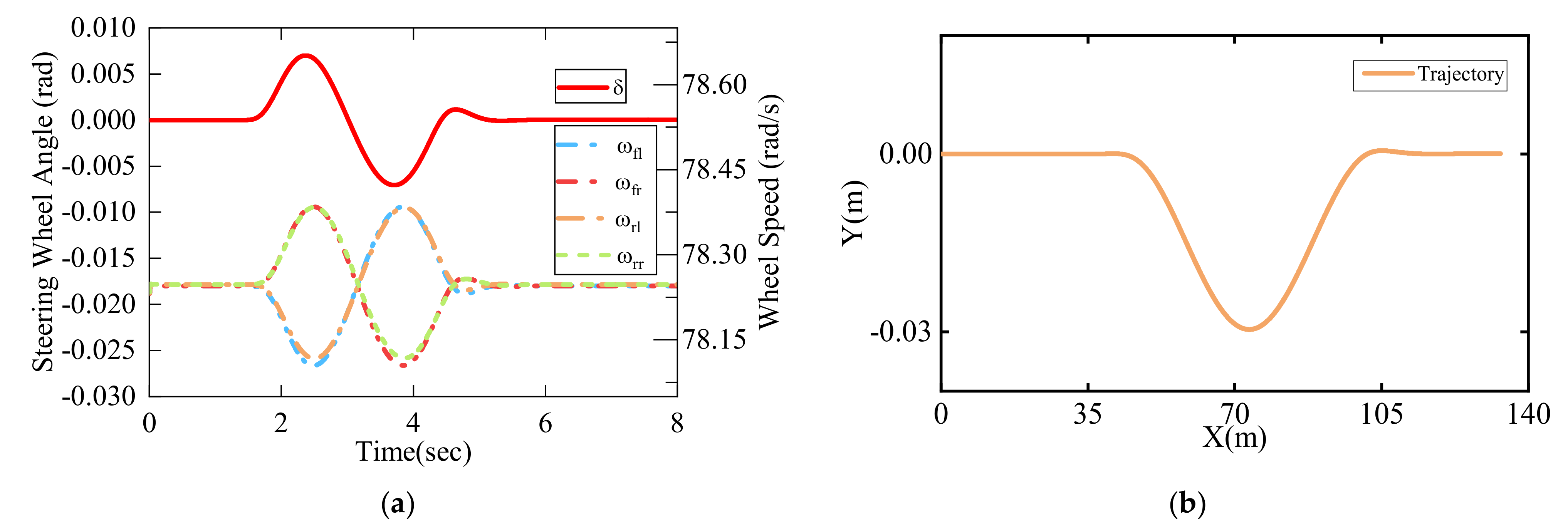
In order to further evaluate the effectiveness of the algorithm under a variety of operating conditions, the algorithm is evaluated using a sinusoidal steering condition, where the initial vehicle speed is set to 80 km/h and the adhesion coefficient of the road surface is set to 0.85. The corresponding system inputs to the observer are shown in Figure 6, and the simulation results of the corresponding SCKF algorithm are compared with those of the IMM-SCKF algorithm as shown in Figure 7.

As shown in Figure 7a, which is a comparison of the longitudinal observation results, both algorithms have high observation accuracy, but the IMM-SCKF algorithm is able to estimate with smaller following error at higher vehicle speed conditions. In Figure 7b lateral vehicle speed observation, due to the higher vehicle speed, the steering angle is larger at this time, and the tire enters the nonlinear region, and the lateral force calculation result has some error with the real result at this time. Therefore, both observers have certain errors in the steering condition, but the IMM-SCKF algorithm can quickly adjust to a smaller error model output after the steering condition is over, and the error of the SCKF algorithm is about 10% at this time. For yaw rate observation, both IMM-SCKF algorithm and SCKF algorithm have high accuracy, but IMM-SCKF is relatively more resistant to noise, while UKF algorithm has a certain estimation error of about 15% under large steering angle conditions.

4.3. Sinusoidal Steering Combined with Braking Conditions

Under this condition, the initial speed is set to 60 km/h, the road adhesion coefficient is set to 0.85, the brake master cylinder pressure is set to 0.3 Mpa, and the sinusoidal steering angle is input in Carsim. The corresponding input of the observer is shown in Figure 8, and the corresponding comparison of the algorithm results is shown in Figure 9.

As shown in Figure 9a, various algorithms can maintain effective tracking of longitudinal vehicle speed, with the IMM-SCKF algorithm having higher accuracy. In the lateral vehicle speed observation results in Figure 9b, all three algorithms have some errors due to simultaneous braking in vehicle steering, but the IMM-SCKF algorithm can quickly switch to adjust the probability of each model and can maintain a small error output with the reference value. All three algorithms have high accuracy in yaw rate observation, but IMM-SCKF has a small estimation error.

To further evaluate the estimation effectiveness of the two algorithms, the root mean square error (RMSE) was used for quantitative analysis and is calculated as follows:

$${\mathrm{RMSE}}_k(i)=\sqrt{\frac{1}{M}{\displaystyle \sum _{l=1}^M{(x_k^{(l)}(i)-{\widehat{x}}_{k\mid k}^{(l)}(i))}^2}}$$

(52)

The calculated RMSE index are shown in

Table 2. Comparison of RMSE values under two simulation conditions.

Simulation Condition	Parameters	UKF	SCKF	IMM-SCKF
Double-lane change condition	Yaw rate	0.0137	0.0088	0.0007
	Longitudinal velocity	0.0792	0.0622	0.0276
	Lateral velocity	0.0303	0.0298	0.0107
Sinusoidal steering condition	Yaw rate	0.0039	0.0005	0.0003
	Longitudinal velocity	0.0052	0.0007	0.0002
	Lateral velocity	0.0117	0.0099	0.0041
Sinusoidal steering combined with braking condition	Yaw rate	0.0012	0.0011	0.0007
	Longitudinal velocity	0.0364	0.0245	0.0128
	Lateral velocity	0.4052	0.3729	0.1308

.

Based on the data in Table 2, the IMM-SCKF algorithm has lower RMSE values under both operating conditions, according to the above indexes. The IMM-SCKF algorithm has higher observation accuracy than the SCKF and UKF algorithm, and the state observer of the IMM-SCKF algorithm can better adapt to noise uncertainty and can always follow the model output with smaller errors. As can be seen from

Table 3. Comparison of the actual computing time consumed by various algorithms.

Simulation Condition	UKF	SCKF	IMM-SCKF
Double-lane change condition	6.74 s	4.12 s	3.69 s
Sinusoidal steering condition	5.02 s	3.21 s	2.87 s
Sinusoidal steering combined with braking condition	7.32 s	3.88 s	3.67 s

, the SCKF algorithm has lower computational complexity and shorter simulation time than the UKF algorithm, while the IMM-SCKF also shows better computational performance, the actual consumption of simulation time is the shortest under various operating conditions, and the algorithm has better real-time performance while ensuring accuracy.

5. Conclusions

In this paper, we propose an interacting multiple model based on square root cubature Kalman filter algorithm and apply the algorithm to distributed drive electric vehicle observation. Experimental validation of the algorithm was carried out using double-lane change condition with a sinusoidal condition and sinusoidal steering combined with a braking condition, which can perform accurate estimation of vehicle state based on less on-board sensor information and can effectively resist the effect of noise. The model was designed based on the 3-DOF vehicle dynamics and nonlinear brush tire model. The interacting multiple model approach allows multiple observers with different noise covariance matrices to interact with one another, improving the overall algorithm’s performance against noise uncertainty to some extent, and the observer can always choose the sub-model with smaller errors for the state output. The co-simulation results show that the IMM-SCKF algorithm can estimate the vehicle longitudinal, lateral, and transverse sway motion states well, and its estimated information can provide accurate and reliable information for the active safety control system.

Future research could include developing a hardware-in-the-loop simulation platform for vehicle state observation, studying vehicle models with more degrees of freedom and parameter estimation, and conduct hardware-in-the-loop simulation and real-vehicle tests to further evaluate the algorithm in terms of real-time and accuracy.

References

- Song, R.; Fang, Y. Vehicle state estimation for INS/GPS aided by sensors fusion and SCKF-based algorithm. Mech. Syst. Signal. Process. 2021, 150, 107315. [Google Scholar] [CrossRef]
- Heidfeld, H.; Schünemann, M. Optimization-Based Tuning of a Hybrid UKF State Estimator with Tire Model Adaption for an All-Wheel Drive Electric Vehicle. Energies 2021, 14, 1396. [Google Scholar] [CrossRef]
- Fnadi, M.; Plumet, F.; Benamar, F. Nonlinear Tire Cornering Stiffness Observer for a Double Steering Off-Road Mobile Robot. In Proceedings of the 2019 International Conference on Robotics and Automation (ICRA), Montreal, QC, Canada, 20–25 May 2019. [Google Scholar]
- Fnadi, M.; Du, W.; Plumet, F.; Benamar, F. Constrained Model Predictive Control for Dynamic Path Tracking of a Bi-steerable Rover on Slippery Grounds. Control Eng. Pract. 2020, 107, 104693. [Google Scholar] [CrossRef]
- Kang, H.-S.; Kim, Y.-T.; Hyun, C.-H.; Park, M. Generalized Extended State Observer Approach to Robust Tracking Control for Wheeled Mobile Robot with Skidding and Slipping. Int. J. Adv. Robot. Syst. 2013, 10, 155. [Google Scholar] [CrossRef]
- Song, Y.; Shu, H.; Chen, X. Chassis integrated control for 4WIS distributed drive EVs with model predictive control based on the UKF observer. Sci. China Technol. Sci. 2020, 63, 397–409. [Google Scholar] [CrossRef]
- Liu, Y.H.; Li, T.; Yang, Y.; Ji, X.; Wu, J. Estimation of tire-road friction coefficient based on combined APF-IEKF and iteration algorithm. Mech. Syst. Signal Process. 2017, 88, 25–35. [Google Scholar] [CrossRef]
- Reina, G.; Messina, A. Vehicle Dynamics Estimation via Augmented Extended Kalman Filtering. Measurement 2019, 133, 383–395. [Google Scholar] [CrossRef]
- Cheng, Q.; Correa Victorino, A.; Charara, A. A new nonlinear observer using unscented Kalman filter to estimate sideslip angle, lateral tire road forces and tire road friction coefficient. In Proceedings of the 2011 IEEE Intelligent Vehicles Symposium (IV), Baden-Baden, Germany, 5–9 June 2011; pp. 709–714. [Google Scholar]
- Wang, Z.; Qin, Y.; Hu, C.; Dong, M.; Li, F. Fuzzy Observer-Based Prescribed Performance Control of Vehicle Roll Behavior via Controllable Damper. IEEE Access. 2019, 7, 19471–19487. [Google Scholar] [CrossRef]
- Jeong, D.; Kim, S.; Lee, J.; Choi, S.B.; Kim, M.; Lee, H. Estimation of Tire Load and Vehicle Parameters Using Intelligent Tires Combined with Vehicle Dynamics. IEEE Trans. Instrum. Meas. 2021, 70, 1–12. [Google Scholar] [CrossRef]
- Henning, K.U.; Speidel, S.; Gottmann, F.; Sawodny, O. Integrated lateral dynamics control concept for over-actuated vehicles with state and parameter estimation and experimental validation. Control Eng. Pract. 2021, 107, 104704. [Google Scholar] [CrossRef]
- Miao, Y.; Zhang, L.; Zhou, X. BeiDou/SINS tightly-coupled integrated navigation algorithm based on federated squared-root CKF. In Proceedings of the 2019 14th IEEE International Conference on Electronic Measurement & Instruments (ICEMI), Changsha, China, 1–3 November 2019; pp. 1493–1499. [Google Scholar]
- Shen, C. Seamless GPS/Inertial Navigation System Based on Self-Learning Square-Root Cubature Kalman Filter. IEEE Trans. Ind. Electron. 2021, 68, 499–508. [Google Scholar] [CrossRef]
- Wan, W.; Feng, J.; Song, B.; Li, X. Huber-Based Robust Unscented Kalman Filter Distributed Drive Electric Vehicle State Observation. Energies 2021, 14, 750. [Google Scholar] [CrossRef]
- Zhang, Z. Correction adaptive square-root cubature Kalman filter with application to autonomous vehicle target tracking. Meas. Sci. Technol. 2021, 32, 14. [Google Scholar] [CrossRef]
- Cheng, S.; Li, L.; Chen, J. Fusion Algorithm Design Based on Adaptive SCKF and Integral Correction for Side-Slip Angle Observation. IEEE Trans. Ind. Electron. 2018, 65, 5754–5763. [Google Scholar] [CrossRef]
- Ping, X. Adaptive estimations of tyre–road friction coefficient and body’s sideslip angle based on strong tracking and interactive multiple model theories. Proc. Inst. Mech. Eng. Part D J. Automob. Eng. 2020, 234, 095440702094141. [Google Scholar] [CrossRef]
- Huang, J.; Zhang, H.; Wu, S.; Tang, G.; Bao, W. An Interacting-Multiple-Model Method for Tracking a Hypersonic Glide Target. In Proceedings of the 2020 Chinese Control and Decision Conference (CCDC), Hefei, China, 22–24 August 2020; pp. 1702–1707. [Google Scholar]
- Liu, H.; Zhou, Z.; Yang, H. Tracking maneuver target using interacting multiple model-square root cubature Kalman filter based on range rate measurement. Int. J. Distrib. Sens. Netw. 2017, 13, 1550147717747848. [Google Scholar] [CrossRef] [Green Version]
- Song, R.; Chen, X.; Fang, Y.; Huang, H. Integrated navigation of GPS/INS based on fusion of recursive maximum likelihood IMM and Square-root Cubature Kalman filter. ISA Trans. 2020, 105, 387–395. [Google Scholar] [CrossRef] [PubMed]
- Jin, X.; Yin, G. Estimation of lateral tire–road forces and sideslip angle for electric vehicles using interacting multiple model filter approach. J. Franklin Inst. 2015, 352, 686–707. [Google Scholar] [CrossRef]
- Ahn, C.; Tseng, H.E. Robust estimation of road friction coefficient using lateral and longitudinal vehicle dynamics. Vehicle Syst. Dyn. 2012, 50, 1–25. [Google Scholar] [CrossRef]
- Zhang, A.; Bao, S.; Bi, W.; Yuan, Y. Low-cost adaptive square-root cubature Kalman filter for systems with process model uncertainty. J. Syst. Eng. Electron. 2016, 27, 945–953. [Google Scholar] [CrossRef]
- Ruggaber, J.; Brembeck, J. A Novel Kalman Filter Design and Analysis Method Considering Observability and Dominance Properties of Measurands Applied to Vehicle State Estimation. Sensors 2021, 21, 4750. [Google Scholar] [CrossRef] [PubMed]
- Chen, S.; Li, C.-F.; Chen, X.; Li, L.; Wu, X.-H.; Fan, Z.-X. A hierarchical estimation scheme of tire-force based on random-walk SCKF for vehicle dynamics control. J. Franklin Inst. 2020, 357, 13964–13985. [Google Scholar] [CrossRef]
- Li, Y.; Jia, Y. Stereovision-based Relative Motion Estimation Between Non-cooperative spacecraft. In Proceedings of the 2019 Chinese Control Conference (CCC), Guangzhou, China, 27–30 July 2019. [Google Scholar]
Figure 1.
Planar vehicle model.
Figure 2.
Lateral force calculation of brush tire model and MF tire model.
Figure 3.
IMM-SCKF flow chart.
Figure 4.
Double-lane change condition (a) observer input, including front wheel angle and four-wheel speed; (b) vehicle trajectory.
Figure 5.
Simulation results of vehicle state under double-lane change condition: (a) longitudinal velocity; (b) lateral velocity; (c) yaw rate; (d) probability of each IMM’s model.
Figure 6.
Sinusoidal steering condition: (a) observer input, including front wheel angle and four-wheel speed; (b) vehicle trajectory.
Figure 7.
Simulation results of vehicle state under sinusoidal steering condition: (a) longitudinal velocity; (b) lateral velocity; (c) yaw rate; (d) probability of each IMM’s model.