SMM: Leveraging Metadata for Contextually Salient Multi-Variate Motif Discovery

Abstract

A common challenge in multimedia data understanding is the unsupervised discovery of recurring patterns, or motifs, in time series data. The discovery of motifs in uni-variate time series is a well studied problem and, while being a relatively new area of research, there are also several proposals for multi-variate motif discovery. Unfortunately, motif search among multiple variates is an expensive process, as the potential number of sub-spaces in which a pattern can occur increases exponentially with the number of variates. Consequently, many multi-variate motif search algorithms make simplifying assumptions, such as searching for motifs across all variates individually, assuming that the motifs are of the same length, or that they occur on a fixed subset of variates. In this paper, we are interested in addressing a relatively broad form of multi-variate motif detection, which seeks frequently occurring patterns (of possibly differing lengths) in sub-spaces of a multi-variate time series. In particular, we aim to leverage contextual information to help select contextually salient patterns and identify the most frequent patterns among all. Based on these goals, we first introduce the contextually salient multi-variate motif ($\mathtt{CS}$-$\mathtt{motif}$) discovery problem and then propose a salient multi-variate motif (SMM) algorithm that, unlike existing methods, is able to seek a broad range of patterns in multi-variate time series.

1. Introduction

A key challenge in multimedia (e.g., video [1,2] and sensor [3]) data mining is the unsupervised discovery of recurring patterns in time series data. In this paper, we focus on the efficient and accurate identification of frequently recurrent patterns, motifs, in multi-variate time series. The discovery of such motifs in uni-variate time series is a well-studied problem [4]. However, in most multimedia applications, the resulting time series are multi-variate; therefore, applications require multi-variate motifs.

1.1. Multi-Variate Motif Search

As further discussed in the related works section, there are several proposals for multi-variate motif discovery [5]. In [6], the multi-variate time series is first projected into a single dimension using principle component analysis (PCA) and then uni-variate motifs are identified on this representation. In [7], multi-dimensional motifs are grouped based on predefined temporal proximity using neighbor distance. The authors of [8] first convert each time-series into a symbolic representation and seek co-occurring motif instances across variates. The authors of [9] construct a data structure known as matrix-profile for each variate and then cluster temporally overlapping sub-sequences across variates.

1.2. Key Questions

In this paper, we note that, in addition to relying on different data structures and algorithms to seek motifs, existing algorithms make very constraining assumptions about what constitutes a re-occurring multi-variate pattern. While most authors agree that a pattern does not need to be exactly repeated and some variations can be allowed, several questions remain:

• Do the instances of a recurring pattern need to cover the same sub-set of variates (Figure 1, dribbling action), or can they occur on a different subsets of variates (Figure 2, climbing action)?
• Can the re-occurring pattern stretch or shrink in time, due to variations in speed, or does it have to be, more or less, the same length as the original?
• Is there a lower bound on the number of times a pattern repeats, before being marked as a motif, or is repeating once sufficient?
• Does any re-occurring pattern count as a motif, or do these patterns have to satisfy some additional constraints, such as being concentrated on a set of variates which are contextually related (such as sensors on the same arm)?

Most existing algorithms provide only answers to a subset of these questions; the repeated pattern is assumed to occur on the same set of variates, the duration of the repeated instances is constrained to be more or less identical and any pair of repeating patterns is returned as a motif, irrespective of whether the variates have any contextually relevant relationships.

1.3. Our Contributions: Contextually Salient Motifs

In contrast to prior works, in this paper, we aim to address a relatively broader form of multi-variate pattern detection problems. In particular, we argue that a useful definition of multi-variate motifs must allow for significant variations in the duration as well as in the subset of variates that are involved in the repeated pattern. Therefore, we seek frequently occurring patterns that are possibly of differing lengths and possibly covering different variates.

While relaxing the above constraints in motif discovery, we observe that not all repeated patterns are useful and argue that a stronger constraint is needed to filter out meaningless repetitions to ensure that the motifs have minimal noise and redundancy in the detected patterns. In particular, we introduce contextually salient motifs ($\mathtt{CS}$-$\mathtt{motif}$s) consisting of multi-variate patterns that are meaningful, considering the available metadata (or context). While such metadata is often available in many multimedia applications (i.e., multimedia sensing and motion capture—see Figure 3), unfortunately, existing motif extraction algorithms largely ignore them. Therefore, a key benefit of the proposed contextually salient motifs (SMM) algorithm is that, unlike existing uni-variate methods, the proposed scheme will be able to seek a broad range of patterns in commonly occurring multi-variate time series data.

Given these, we first formally define the frequent, contextually salient, multi-variate motif discovery problem (Section 3); then, in Section 4, we introduce a salient multi-variate motif (SMM) algorithm for seeking such motifs. The proposed algorithm first identifies contextually salient multi-variate patterns in relevant sub-spaces of the given time series. These contextually salient patterns are then appropriately clustered and pruned to identify frequently occurring patterns. The experimental evaluations, presented in Section 5, illustrate the effectiveness of the proposed SMM algorithm in identifying frequent, contextually salient, multi-variate motifs ($\mathtt{CS}$-$\mathtt{motif}$s) in a given multi-variate time series.

2. Related Works

In this section, we first discuss related work in motif discovery and then focus on the literature on multivariate motif discovery, which is also the main focus of this paper.

2.1. Motifs

Motif discovery is an important task in multimedia analysis, motivated by the recent increase in applications with sensory data [7] and other sequence-based applications, such as gene analysis [11]. The authors of [12] defined the problem as searching for the most common non-overlapping subsequences. Motifs, if used properly, have been shown to be a powerful tool for various time series analysis applications, such as summarization, classification and visualization [13,14,15,16,17]. Ref. [5] is a survey on the recent motif discovery approaches. The two main research challenges in motif discovery are scalability and accuracy. For uni-variate time series, most of the works in literature focus on the problem of computational complexity and include symbolic signatures (i.e., approximate representations), such as SAX [18], and other approximate methods to locate motifs. For example, the authors of [19] proposed to use a random projection-based algorithm originally used for analyzing DNA sequences. A second scalability challenge regards the memory requirement; many of the existing algorithms are quadratic in space and time, as a collision matrix needs to be maintained in the main memory [19]. The authors of [20] showed that the motif discovery can be affected by slight deformations in the data (e.g., linear stretching of the pattern length) and introduced a scaling-invariant algorithm, building on the approach proposed in [19], but using scale-free distance computation. The impact of having a multi-scale approach to indexing was investigated in [21], where it is allowed to have motif signatures (SAX words) of different resolutions (as opposed to considering motifs of different lengths). Recently, researchers have also investigated related problems, including finding a few top motifs, and developed pruning algorithms to boost efficiency (top-1 motifs [22] and top-n motifs [23]). Other approaches include considering a priori information in terms of the probable locations of the motifs [24], in particular leveraging a change point detection algorithm to associate a change score to each point in the time series. A matrix profile is a data structure that supports efficient all-pair-similarity search in uni-variate time series [25]; intuitively, the matrix profile data structure enables one to identify the most similar pairs of subsequences (of a given length) in a given time series.

2.2. Multi-Variate Motifs

The state-of-the-art approaches for multi-variate (multi-dimensional) motif discovery often belong to one of two categories. (a) Symbolization: For searching uni-variate motifs, first convert the input time series data into a symbolic form and then apply symbolic mining techniques to discover motifs [18]. This can also be extended to multi-variate series by applying symbolization onto vectors. In [6], the multi-variate time series is first projected into a single dimension using PCA; then, the SAX representation is extracted and, finally, the motifs on this uni-variate series are discovered using minimum description language (MDL [26]). (b) Direct search avoids the symbolization process and motifs are searched directly on the time series data. In [27], once single variate motifs are identified, multi-variate motifs are constructed combining those single variate motifs based on their overlaps in time and variates. In [6,28,29], the authors leverage logical (AND and OR) operators to concatenate collision matrices extracted from sub-sequence matching in each variate. This helps discover motifs of same length, but has poor accuracy if a pattern can be stretched or contracted. Other approaches include similarity matrix-based approaches and density-estimation-based techniques [30,31].

Motif search in sub-spaces is an expensive process, as the potential number of sub-spaces in which a pattern can occur increases exponentially with the number of variates. A possible simplification of the multi-variate motif search is to seek concurrent motifs across all dimensions. In [7], the motif grouping process is based on a predefined temporal proximity using neighbor distance. After the identification of neighbor data points using scope information along the temporal dimension, motifs computed from these neighbor points are stored in a motif bag (treated as potential multi-dimensional motifs). An alternative model is to track recurring groups of temporal relations among co-occurring motif instances where SAX is first applied on each dimension, followed by a grammar induction approach to identify re-occurring patterns [8].

In [9], the concept of matrix profiles introduced in [25] was extended to multi-variate time series. The algorithm essentially constructs matrix profiles separately for each variate; then, it clusters, in a bottom-up fashion, temporally overlapping pairs of sub-sequences across different variates to find the most similar multi-variate subsequences in the data. While this algorithm is quite efficient, it has several limitations. Firstly, the algorithm returns pairs of similar sub-sequences and, to identify the most frequent patterns, one still has to do additional post-processing. Secondly, the algorithm takes the length of the sub-sequence as given; further, it is limited with patterns that are of the same length and are re-occurring on the same set of variates.

3. Problem Definition

In this section, we formally define the frequently recurring, contextually salient, multi-variate motif search problem.

3.1. Uni-Variate Motifs and Local Saliency

We first start with uni-variate definitions.

Definition 1 (Uni-Variate Time Series).

A uni-variate time series$\mathcal{T}=(d_1,d_2,\dots ,d_N)$is a temporally ordered sequence of values. Here, N denotes the length of the time series and$d_i\in \mathcal{R}$. We also denote the center of the time series as$center\left(\mathcal{T}\right)=\lfloor \frac{N+1}{2}\rfloor$.

Definition 2 (Subsequence of a Time Series).

A subsequence$\mathcal{S}=(d_i,d_{i+1},\dots ,d_j)$of a time series$\mathcal{T}$(of length N) is a consecutive subset of values from$\mathcal{T}$; here, we have$1\le i<j\le N$, while$d_i$and$d_j$are the observations at$t_i$and$t_j$, respectively. We denote the center of the subsequence as$center\left(\mathcal{S}\right)=\lfloor \frac{j+i}{2}\rfloor$and the length of the subsequence as$length\left(\mathcal{S}\right)=j-i+1$.

Now, we define local salience value of a subsequence relative to a distance function Δ.

Definition 3 (Local Salience Value of a Subsequence).

Given a subsequence$\mathcal{S}=(d_i,d_{i+1},\dots ,d_j)$of a time series$\mathcal{T}$(of length N), we refer to the value

$$ls\left(\mathcal{S}\right)=\Delta (\mathcal{S},half\left({\mathcal{S}}^{\top }\right)).$$

as the local salience value of the subsequence$\mathcal{S}$. Here,

• ${\mathcal{S}}^{\top }$is a sub-sequence of double length, centered at the same time instance as$\mathcal{S}$(i.e.,$center\left(\mathcal{S}\right)=center\left({\mathcal{S}}^{\top }\right)$);
• $half\left(\right)$is a function that subsamples a time series into half its length.

Intuitively, high local salience of a subsequence $\mathcal{S}$ implies that it is well defined in (in the sense of being different from) its temporal neighborhood (Figure 4). Note that this definition is very general and does not impose any constraints on the nature of the Δ function or the lengths of the subsequences.

Then, a locally salient subsequence has the highest local salience value in its immediate neighborhood in time and temporal scale.

Definition 4 (Locally Salient Subsequence).

Let subsequence${\mathcal{S}}_{c,l}=(d_i,d_{i+1},\dots ,d_j)$of a time series$\mathcal{T}$be such that$c=center\left(\mathcal{S}\right)$and$l=length\left(\mathcal{S}\right)$.${\mathcal{S}}_{c,l}$is said to be a locally salient subsequence if

$$ls\left({\mathcal{S}}_{c,l}\right)>MAX\left\{\begin{array}{ccc}ls\left({\mathcal{S}}_{c-1,l}^{*}\right),& \left({\mathcal{S}}_{c,l}^{*}\right),& ls\left({\mathcal{S}}_{c+1,l}^{*}\right)\\ ls\left({\mathcal{S}}_{c-1,l}\right),& & ls\left({\mathcal{S}}_{c+1,l}\right)\\ ls\left({\mathcal{S}}_{c-1,l}^{+}\right),& \left({\mathcal{S}}_{c,l}^{+}\right),& ls\left({\mathcal{S}}_{c+1,l}^{+}\right)\end{array}\right\},$$

where

• ${\mathcal{S}}^{*}=double\left(S^{\perp }\right)$;
• ${\mathcal{S}}^{+}=half\left(S^{\top }\right)$;
• ${\mathcal{S}}^{\top }$is a sub-sequence of double length, centered at the same time instance as$\mathcal{S}$(i.e.,$center\left(\mathcal{S}\right)=center\left({\mathcal{S}}^{\top }\right)$);
• ${\mathcal{S}}^{\perp }$is a sub-sequence of half length, centered at the same time instance as$\mathcal{S}$;
• $double\left(\right)$is a function that supersamples a time series into double length;
• $half\left(\right)$is a function that subsamples a time series into half its length.

Intuitively, a subsequence is locally salient if it has the highest local salience value among all its neighboring subsequences in time and scale. Given this, we now can define recurring sub-sequences that are locally salient with respect to their temporal contexts.

Definition 5 (Recurring LS-Pattern).

A locally salient sub-sequence ${\mathcal{S}}_0$ of a time series $\mathcal{T}$ of length $l\le N$ is said to be a $(k,l,ϵ)$-recurring locally salient (LS) sub-sequence, relative to a distance function Δ, if there are $k-1$ other locally salient sub-sequences ${\mathcal{S}}_1,\dots ,{\mathcal{S}}_{k-1}$ of $\mathcal{T}$ such that

$${\forall }_{1\le i\le k-1}\Delta ({\mathcal{S}}_0,{\mathcal{S}}_i)\le ϵ$$

and, for all $0\le i\le k-1$, ${\mathcal{S}}_i$ $length\left({\mathcal{S}}_i\right)\ge l$. Then, the set $recPat=\{{\mathcal{S}}_0,\dots ,{\mathcal{S}}_{k-1}\}$ is referred to as a $(k,l,ϵ)$-recurring LS-pattern.

This leads us to the definition of locally salient motifs on univariate time series.

Definition 6 (LS-Motif).

Let the set $recPat=\{{\mathcal{S}}_0,\dots ,{\mathcal{S}}_{k-1}\}$ be a $(k,l,ϵ)$-recurring LS-pattern of time series T. We refer to this as a $(k,l,ϵ)$ LS-Motif if the set is maximal, i.e., there is no $(k^{\prime },l,ϵ)$-recurring LS-pattern $recPa{t}^{\prime }$ such that $k^{\prime }>k$ and $recPa{t}^{\prime }\supset recPat$.

Note that, if a motif is locally salient with respect to its local temporal context, then it is not only maximal in terms of the size of the set of repeating patterns, but it is also well defined in its immediate temporal neighborhood.

3.2. Multi-Variate Motifs and Contextual Saliency

We now extend the above definitions to multi-variate time series.

Definition 7 (Multi-Variate Time Series and their Context).

A Multi-Variate Time Series$\mathbb{T}=({\mathcal{T}}_1,{\mathcal{T}}_2,\dots ,{\mathcal{T}}_M)$is a set of M uni-variate time series with the same sampling rate and the same length N. We denote the temporal length of$\mathbb{T}$as$length\left(\mathbb{T}\right)$and its variate width (i.e., the number of variates) as$width\left(\mathbb{T}\right)$($=M)$. We refer to C, an$M\times M$matrix denoting the known relationships among the M variates, as the context of$\mathbb{T}$.

The contextual relationship matrix, C, is application-specific and can be visualized in the form of a graph capturing the relationships among variates, as visualized in Figure 2 and Figure 3. Note that, if such contextual relationships are not known, then $C={\mathbf{1}}_{M\times M}$, i.e., it is a matrix where all variates are equally related to all other variates.

Definition 8 (Subsequence of a Multi-Variate Series).

Let $\mathbb{T}$ be a multi-variate time series with M variates of length N. A multi-variate subsequence $\mathbb{S}$ of this series is a set of P uni-variate subsequences ${\mathcal{S}}_1,\dots ,{\mathcal{S}}_P$ such that each subsequence ${\mathcal{S}}_i$ starts at the same time and has the same length as the other subsequences, but is on a distinct variate set relative to the rest. We denote the temporal length of $\mathbb{S}$ as $length\left(\mathbb{S}\right)$ and its variate width as $width\left(\mathbb{S}\right)=P$. We further define the temporal scope $tScope\left(\mathbb{S}\right)$ of the subsequence as the temporal interval from the first time instant to the last. Similarly, the variate scope, $vScope\left(\mathbb{S}\right)$, of the subsequence is defined as the set of P variates that make up this multi-variate subsequence.

Given the above definitions of multi-variate time series and sub-sequences and a multi-variate distance function ${\Delta }_C\left(\right)$, which also takes into account the variate context C, when comparing multi-variate sub-sequences, we can extend the definitions of salience to multi-variate data.

Definition 9 (Contextual Salience Value of a Multi-Variate Subsequence).

Let subsequence $\mathbb{S}$ be a multi-variate subsequence of $\mathbb{T}$. The contextual salience value of $\mathbb{S}$ is defined as

$$\begin{array}{c}\hfill cs\left(\mathbb{S}\right)={\Delta }_C(\mathbb{S},compres{s}_C({\mathbb{S}}^{\top ,C},vScope\left(\mathbb{S}\right))),\end{array}$$

where

• ${\mathbb{S}}^{\top ,C}$ is a multi-variate subsequence with the same center and length as $\mathbb{S}$, but has twice as large a variate width topologically centered around $vScope\left(\mathbb{S}\right)$, based on the variate context C;
• $compres{s}_C(\mathbb{S},v\_scope)$ is a function that compresses a given multi-variate time series from its original variate scope down to the variate scope defined by $v\_scope\subseteq vScope\left(\mathbb{S}\right)$.

Intuitively, high contextual salience of a subsequence $\mathcal{S}$ implies that it is well defined in (in the sense of being different from) its contextual neighborhood. Note that this definition is very general and does not impose any constraints on the nature of the ${\Delta }_C$ function or the definitions of ${\mathbb{S}}^{\top ,C}$ and $compres{s}_C(\mathbb{S},v\_scope)$.

Then, a contextually salient subsequence has the highest local salience and contextual salience values in its immediate neighborhood in time and variate scales and we can define recurring sub-sequences that are contextually salient with respect to their temporal and variate contexts.

Definition 10 (Recurring CS-Pattern).

A contextually salient sub-sequence ${\mathbb{S}}_0$ of a time series $\mathbb{T}$ of length $l\le N$ is said to be $(k,l,ϵ)$-recurring locally salient (LS) sub-sequence, relative to a distance function Δ if there are $k-1$ other contextually salient sub-sequences ${\mathbb{S}}_1,\dots ,{\mathbb{S}}_{k-1}$ of $\mathbb{T}$ such that

$${\forall }_{1\le i\le k-1}\Delta ({\mathbb{S}}_0,{\mathbb{S}}_i)\le ϵ$$

and, for all $0\le i\le k-1$, $length\left({\mathbb{S}}_i\right)\ge l$. Then, the set $recPat=\{{\mathbb{S}}_0,\dots ,{\mathbb{S}}_{k-1}\}$ is referred to as a $(k,l,ϵ)$-recurring CS-pattern.

Then, the definition of contextually salient motifs (or $\mathtt{CS}$-$\mathtt{motif}$s) trivially follows from this.

Definition 11 ($\mathtt{CS}$-$\mathtt{motif}$).

Let the set $recPat=\{{\mathbb{S}}_0,\dots ,{\mathbb{S}}_{k-1}\}$ be a $(k,l,ϵ)$-recurring CS-pattern of the multi-variate time series $\mathbb{T}$. We refer to this as a$(k,l,ϵ)$ $\mathtt{CS}$-$\mathtt{motif}$if the set is maximal, i.e., there is no $(k^{\prime },l,ϵ)$-recurring CS-pattern $recPa{t}^{\prime }$ such that $k^{\prime }>k$ and $recPa{t}^{\prime }\supset recPat$.

Note that, depending on how the distance function ${\Delta }_C$ deals with variate alignment (e.g., whether it enforces that the sub-sequences have the same variate scopes and how it takes into account the contextual information C), we can obtain different types of $\mathtt{CS}$-$\mathtt{motif}$s (Figure 1 and Figure 2).

3.3. Problem Statement

We now introduce the problem we address in this paper.

Problem 1 ($\mathtt{CS}$-$\mathtt{motif}$ Discovery in Multi-Variate Time Series).

Let $\mathbb{T}$ be a multi-variate time series (with variate context C). Let l denote the size of the smallest temporal scope of the target motifs and let ϵ be the similarity bound as defined above. Given these, let $\mathcal{M}$ be the set of all $(k_i,l,ϵ)$-motifs, where $k_i$ denotes the recurrence counts of the pattern in $recPa{t}_i\in \mathcal{M}$. Then, our goal is to identify $(k_i,l,ϵ)$-motifs (or $\mathtt{CS}$-$\mathtt{motif}$s) with the highest recurrence counts in $\mathcal{M}$.

4. SMM: Contextually Salient Multi-Variate Motif ($\mathtt{CS}$-$\mathtt{motif}$) Discovery

In this section, we present a novel approach to identify frequently recurring, contextually salient, multi-variate motifs. To deal with the underlying complexity of the problem and also to achieve the necessary flexibility in the type of motifs we are able to discover, we propose a salient multi-variate subsequence (SMS)-based motif-search mechanism (Figure 5). The proposed motif extraction process consists of two major steps. (a) Multi-variate pattern extraction and description: Salient multi-variate patterns that represent the areas of multi-variate time series with high local saliency are identified. Here, a key challenge is to consider the context information to identify multi-variate features (of different temporal lengths and variate scopes) that are contextually meaningful (Section 4.1). (b) Multi-variate pattern clustering and pruning: In this step, we cluster patterns obtained in the previous step into recurring patterns. Since the sizes and the numbers of the recurring patterns are not known ahead of time, we need to leverage an adaptive clustering strategy, which not only automatically identifies the number of similarity clusters in the data, but also prunes away those multi-variate patterns that do not belong to any of the identified clusters. We discuss this process in Section 4.2.

4.1. Salient Multi-Variate Sub-Sequences (SMSs)

We note that a significant amount of waste in processing can be avoided and noise can be reduced if motif search can be directed towards parts of a given time series that are likely to contain contextually interesting motifs. Furthermore, we argue that time series data often carry structural evidences in the form of salient temporal features and that these can help focus the motif search process on parts of the time series that may contain contextually salient patterns. The proposed salient multi-variate motif (SMM) algorithm locates salient multi-variate temporal sub-sequences (of varying sizes) using a two-step scale-invariant feature search mechanism. In its first step, the algorithm creates scale-space of the given multi-variate time series which reflects its varying granularities; then, it identifies multi-variate subsequences where differences between the sub-sequent time and/or variate granularities are large. In its second step, the algorithm selects, among these sub-sequences, those that are likely to correspond to intervals with interesting patterns and extracts small-footprint descriptors for each of these salient sub-sequences. This approach has several advantages:

• Firstly, the scale-space extrema detection process in the first step ensures that only those subsequences that are significantly different from their neighbors (both in time and variates) are considered as candidate patterns for motifs. Consequently, the overall efficiency of the process is significantly improved by being selective during motif search.
• Secondly, since the process identifies subsequences of different temporal and variate scopes, we can potentially avoid fixing the motif patterns’ sizes in advance.
• The process can also take into account the contextual information that may describe the relationships among the variates.

However, enabling these advantages requires an efficient multi-scale search mechanism to locate salient multi-variate sub-sequences of a given multi-variate time series. In particular, we search for these sub-sequences using an SIFT-like [32,33] process that also takes into account the contextual information such as the metadata graph associated with the variates of the series (Figure 3).

4.1.1. Scale-Spaces of Multi-Variate Time Series

Intuitively, each contextually salient feature $f_i$ extracted from a multi-variate time series is a triple $\langle T_i,V_i,D_i\rangle$, where $T_i=[t_{i,start},t_{i,end}]$ is a time interval (i.e., temporal scope), $V_i$ is a subset of the variates that make up the time series (i.e., variate scope) and $D_i$ is a fixed-length vector describing the local gradient distribution as a function of the underlying metadata. The algorithm to identify these sub-sequences relies on a two-step process. The first stage identifies salient multi-variate sub-sequences across multiple scales (created in a way that takes into account the relationships among the variates). To achieve this, a scale-space representation of the multi-variate series is constructed through iterative smoothing (across time and metadata graph) which creates different resolutions of the input series (Figure 6); then, sub-sequences of interest with the largest variations with respect to their neighbors in both time and variates are located on this scale-space. Once these multi-variate sub-sequences are identified, a gradient histogram is associated to each sub-sequence as a descriptor to support indexing and search.

Temporal and Variate Smoothing

As we can see in Figure 6, the process requires the series to be repeatedly smoothed across both time and variates. While Gaussian smoothing across time is a well-understood process (involving the convolution of the time series with a Gaussian filter $G(t,\sigma )=\frac{1}{\sqrt{2\pi }\sigma }{e}^{\frac{-t^2}{2{\sigma }^2}}$ for a smoothing parameter σ), the same cannot be said for smoothing across variates, because, while time is totally ordered (enabling convolution), the graph is not—therefore, convolution filters cannot be applied directly.

We handle this by (a) defining, for each variate $v_l$, two functions $frw{d}_G(v_l,\delta )$ and $bkw{d}_G(v_l,\delta )$, as the forward and backward neighbors of $v_l$ at a distance at most δ on the metadata graph; given these functions, which (partially) order the variates relative to $v_l$, (b) we apply, for each $v_l$, Gaussian smoothing across variates centered around $v_l$ (the values of variates at the same distance from $v_l$ are averaged).

Given a multi-variate time series $\mathbb{T}$ and a metadata graph C, the smoothing process with temporal-smoothing parameter ${\sigma }_t$ and variate smoothing parameter ${\sigma }_v$ results into scale-space $\mathcal{M}$, where the entry $\mathcal{M}[s_t,s_v](t_i,v_j)$ corresponds to the series at time $t_i$ for variate $v_j$, smoothed $s_t$ times temporally and $s_v$ times across variates of graph C. Increasing the smoothing rates along time and along variates reduces the details in the time series by taking into account the available metadata (Figure 7). Once the scale space is created, the contextually salient $\langle s_t,s_v{t}_i,v_j\rangle$ quadruples can be identified by comparing $\mathcal{M}[s_t,s_v](t_i,v_j)$ to its neighbors (across time, variates and both) and by selecting the quadruples with the largest differences from their neighbors. In Section 4.1.2, we further discuss how these contextually salient subsequences are identified.

Descriptor Creation for Multi-Variate Sub-Sequences

Note that each quadruple $\langle s_t,s_v,t_i,v_j\rangle$ represents a temporal interval (i.e., temporal scope, $[t_i-3\times s_t\times {\sigma }_t,t_i+3\times s_t\times {\sigma }_t]$) centered around time instance $t_i$ and a set of variates (i.e., variate scope) centered around variate $v_j$—in other words, each quadruple can be considered as a contextually salient multi-variate sub-sequence of the input time series $\mathbb{T}$. Once these contextually salient sub-sequences are identified, the next step is to create a descriptor for the sub-sequences to enable their comparisons. While these sub-sequences can be compared using any technique (including multi-variate DTW or others, see [34]), in this paper, we again follow an SIFT-like technique and extract a gradient histogram to be used as a local descriptor; in particular, for each contextually salient $\langle s_t,s_v,t_i,v_j\rangle$ quadruple, we consider the neighborhood of $\mathcal{M}[s_t,s_v](t_i,v_j)$ covered by the corresponding temporal and variate scopes and centered around time $t_i$ and variate $v_j$ and, given this neighborhood, the feature descriptor is created as a c-directional gradient histogram of this matrix, sampling the gradient magnitudes around the salient point using a $2a\times 2b$ grid, where a, b and c are user-provided parameters, superimposed on the neighborhood. To give less emphasis to gradients that are far from the point $\langle v_i,t_j\rangle$, a Gaussian weighting function is used to reduce the magnitude of the elements furthest from $\langle v_i,t_j\rangle$. This process leads to a feature descriptor vector of length $2a\times 2b\times c$. The descriptor size must be selected in a way that reflects the temporal characteristics of the time series. If a multi-variate time series contains many similar features, it might be more advantageous to use large descriptors that can better discriminate; these large descriptors would not only include information that describes the corresponding features, but would also describe the temporal contexts in which these features are located.

4.1.2. Identifying Contextually Salient Sub-Sequences

Let $\langle s_t,s_v,t_i,v_j\rangle$ be a quadruple in the state-space visualized in Figure 6. As discussed above, here, $s_t$ and $s_v$ are the two parameters that control the amount of smoothing across time and variates, respectively, and $t_i$ and $v_j$ are the time instance and variate on which a multi-variate sub-sequence is centered. To identify whether this quadruple represents a contextually salient sub-sequence or not, we need to compare it to its 80 ($=3^4-1$) neighbors across time, variates and two scale spaces (with three neighbors along each of these four dimensions). In this paper, we note that we can use two alternative measures of comparison to identify contextually salient sub-sequences, described below.

Smoothing-Based Contextual Saliency

We define smoothing-based local saliency $C{S}_S(s_t,s_v,t_i,v_j)$ as follows:

$$\begin{array}{ccc}\hfill =max& (& \left|\mathcal{M}[s_t+1,s_v](t_i,v_j)-\mathcal{M}[s_t,s_v](t_i,v_j)\right|,\hfill \\ & & \left|\mathcal{M}[s_t,s_v+1](t_i,v_j)-\mathcal{M}[s_t,s_v](t_i,v_j)\right|,\hfill \\ & & \left|\mathcal{M}[s_t+1,s_v+1](t_i,v_j)-\mathcal{M}[s_t,s_v](t_i,v_j)\right|)\hfill \end{array}$$

.

Intuitively, $C{S}_S$ measures the absolute difference between the smoothed entries at different scales around the quadruple $\langle s_t,s_v,t_i,v_j\rangle$. If $C{S}_S(s_t,s_v,t_i,v_j)$ is larger than the $C{S}_S$ values corresponding to some $\Theta \%$ (for some user-provided $\Theta \sim 100$) of the neighbors of the quadruple $\langle s_t,s_v,t_i,v_j\rangle$ in the state space, then we can say that the multi-variate sub-sequence represented by this quadruple is (maximally) different from its neighbors.

Entropy-Based Contextual Saliency

Note that the above definition of local saliency compares the actual values of the series smoothed at different degrees. Alternatively, we can define an entropy-based contextual saliency $C{S}_E(s_t,s_v,t_i,v_j)$ by replacing $\mathcal{M}$ with $\mathcal{E}$, where $\mathcal{E}[s_t,s_v](t_i,v_j)$ is the Shannon entropy defined within the $(3{\sigma }_t,3{\sigma }_v)$ neighborhood of the smoothed (and suitably discretized) series $\mathcal{M}[s_t,s_v]$ around the time instance $t_i$ and variate $v_j$. Since each neighborhood of a smoothed series corresponds to a multi-variate subsequence, intuitively, $C{S}_E$ measures how different the entropy of a given sub-sequence is relative to the version of the series further smoothed in time and/or in variates.

4.2. Frequently Recurring Motif Search

Once the salient multi-variate sub-sequences of the given multi-variate time series are identified and collected, the next step is to cluster these sub-sequences into recurring patterns, a motif bag. Since the number of distinct motifs in the time series or the number of sub-sequences in each of these motifs may not be known ahead of time, we need to leverage an adaptive clustering strategy, which not only automatically identifies the number of similarity clusters in the data, but also prunes away those multi-variate patterns that do not belong to any of the identified clusters.

To search for the matching motifs across the same or different variate groups, we propose the two following strategies under two different scenarios:

(1)

Finding motifs across the same variate groups, by considering all the features extracted from a multi-variate time series. This requires a three-step process: (a) We create groups of features existing in the same or a similar variate scope; the results are clusters of features sharing the same or a similar variate scope. (b) To identify groups of features with similar behaviors, in each of the groups we apply one cluster (adaptive K-means). (c) In each group of these features, a pruning process is applied to clean the outlier instances from the clusters using standard deviation from the feature centroid.

(2)

Targeting motifs across multiple (potentially different) variate groups. Considering all the features extracted from a multi variate time series, we apply the following steps: (a) First, a clustering technique is applied; in our results, we use adaptive K-means. The clustering process would allow us to identify groups of instances with similar behaviors across potentially different variate groups. (b) For each cluster identified, a pruning step is applied, which takes each cluster centroid and the corresponding standard deviation into consideration. This would allow the proposed framework to arrive at bags of motifs, each containing instances from multiple variate sets. (c) The final step is sub-clustering (we group instances in each motif bag $M_i$ having a similar or the same variate scope), which would be applied to the search for motifs existing on the same variate groups.

While any clustering approach (e.g., density-based clustering, such as DBScan [35]) can be used for this purpose, in our implementation, we use an adaptive K-mean strategy, based on the Euclidean distance of the sub-sequence descriptors. Depending on the type of motifs being searched, additional constraints (such as being of a similar length, or being aligned along similar sets of variates) are considered when forming and maintaining the clusters. Intuitively, each of these clusters represents a potential motif. However, these clusters may contain sub-sequences that do not share the same pattern and, thus, do not belong to the corresponding motif. In order to eliminate these spurious sub-sequences, prune outliers from each cluster. More specifically, the pruning step works in the following way: for each cluster ${\mathcal{C}}_h$ we identify the mean descriptor and the standard deviation

$$D_{mean,h}=\underset{subse{q}_i\in C_h}{AVG}\left(D_i\right),$$

$$sde{v}_h=\underset{subse{q}_i\in C_h}{STDEV}(\Delta (D_i,D_{mean,h})),$$

of the distances of the sub-sequences in the cluster from this mean descriptor. Once these are computed, we eliminate any sub-sequence $subse{q}_i$ in $C_h$, such that

$$\Delta (D_i,D_{mean,h})>3\times sde{v}_h.$$

Intuitively, assuming that the cluster represents a single motif pattern and that the distances of the descriptors (corresponding to a motif pattern) from the mean descriptor follow a normal distribution, this would help eliminate those sub-sequences that have less than $0.03\%$ likelihood of being part of the corresponding motif. Once the initial descriptor-based clusters are obtained, we further partition these clusters based on variate overlaps. However, this is an optional step.

A major advantage of this approach is that we can control what type of re-occurring patterns constitute a motif. In particular, in addition to being able to control things such as whether identified motifs have a certain periodicity or an energy (or entropy) difference relative to the whole of the series, we can also control:

• The degree of variate alignment. As we have seen in the Introduction, Figure 1, while, in some applications, we may wish to ensure that the repeating patterns occur on the same set of variates, in some others, it might be acceptable that re-occurring patterns cover different subsets of variates (Figure 2);
• The degree of length alignment. Again, as stated in the Introduction, Figure 1, while, in some applications, we may wish to ensure that the repeating patterns have the same length, in some others, it might be acceptable that re-occurring patterns are of different lengths.

We experimentally validate the above in the next section.

5. Experimental Evaluation

In this section, we report the results of the experiments that aim to assess the effectiveness of the proposed motif search strategy.

5.1. Datasets

To evaluate the proposed motif detection technique, we rely on three datasets—the key characteristics of these datasets are outlined in

Table 1. Characteristics of the datasets.

Dataset	# Variates	# Time Series	# Classes	Contextual Strength
MoCap [10]	62	184	8	high
Building energy [36]	27	100	n/a	high
Birdsong [37]	52	154	8	low

:

• The motion capture (MoCap) dataset [10] consists of movement records from sensors placed on subjects’ bodies as they perform 8 types of tasks. We use the Acclaim-Skeleton-File/Acclaim Motion Capture (ASF/AMC) data format, where the original coordinate readings are converted into 62 joint angles’ data. We treat the readings for each joint angle as a different uni-variate time series. The hierarchical spatial distribution (e.g., left foot, right foot, left leg, etc.) of the joint angles on the body is used to create the underlying correlation matrix used as contextual metadata.
• The building energy dataset consists of energy simulations generated through the EnergyPlus simulation software [36]. In this case, the variate context is defined based on the topology of the building being simulated.
• The BirdSong dataset [37] consists of Mel-frequency cepstral coefficient (MFCC) features for different bird calls. Each MFCC coefficient captures the short-term power spectrum of a sound for a given frequency band. The original dataset contains 13 MFCC coefficients (i.e., variates) for 154 bird calls of 8 classes, with the average time length of 397 time stamps. For our experiments, we convert these into the frequency domain and produce a multi-variate time-series composed of 52 variates. The context is defined in terms of the proximity of the constituent frequencies; in particular, we consider them to be equally spaced on the Mel scale.

Note that, as reported in Table 1, the contextual metadata are more strongly defined for the motion capture and building energy datasets, where the spatial proximity and connections among body and building components are used to capture the context. The contextual metadata is less strongly defined for the birdsong dataset.

Samples of these time series are visualized in Figure 8—note that the repeated patterns are also discernible to the naked eye in these samples.

5.2. Motifs Used as Ground Truth

For a fair evaluation, as is common in the literature, we inject true motifs onto time series generated through random walks. Then, the injected motifs are used as labeled ground truth (Ground truth data are available at https://drive.google.com/drive/folders/1NBvywswb1wzryIwhIW2xiS17ns_xF03J?usp=sharing, accessed on 20 May 2021). In order to ensure that the simulated series are meaningful representations of the original time series, we first compute the average displacement for the series and, at each step of the random walk, we make a move bounded by a percentage of the original average displacement. In the experiments, we considered 10, 25, 50, 75 and 100% average displacement. In addition, we considered a (0–1) random walk where the average displacement was bounded simply by 1 unit (this corresponds to a mostly idle motion pattern).

The ground truth motifs are created and injected as follows:

• First, we identify and extract multi-variate dominant behaviors/patterns in the form of RMT features (robust multivariate time-series feature) from the series in a given dataset.
• Then, we select a random set of distinct patterns to be injected as motifs.
• Next, we generate a set of multi-variate random walks to be used as the motif-free time series; to ensure that the generated series closely match the characteristics of the original series, we perform the following operations:
  • We compute, from each motif pattern, the value of average displacement;
  • We scale the generated random walks to match a specific percentage of the average displacement of the motif patterns for making the motif instances injected consistent within the global behavior over the time series.
• We finally inject the selected patterns onto the created motif-free random walks.

We record, as ground truth, the variates on which the patterns have been injected along with the temporal scopes of the pattern insertions.

Table 2. Experimental settings; default values are highlighted in bold.

Parameters	Values
number of motifs (m)	1, 2, 3
recurrence count (k)	5, 10, 15
length flexibility percentage (f)	50, 75, 100
average displacement scaling percentage	10, 50, 75, 100

provides an outline of the characteristics of the time series that are generated through the above process:

• Number of motifs (m): this is the number of motifs inserted into a single multivariate series;
• Recurrence count (k): this is the number of patterns inserted for each motif;
• Length flexibility (f): for a given motif, we allowed the length of its subsequences to vary—f denotes the lowerbound on the length of the subsequences as a percentage of the original pattern.

In addition to the above, we considered alternative variate alignment and placement strategies for the injected motifs; motifs are inserted either on the original variates (v-aligned; default), or on variates that are structurally similar to the original ones (v-structure).

In the experiments reported in this section, we compare the proposed SMM algorithm to one of the most recent multi-variate motif proposals, the matrix-profile strategy [25], which we refer to, in this section, as matrix profile with clustering (MPC). Note that the original matrix-profile algorithm identifies recurring pairs of multi-variate subsequences; given all the recurring sub-sequences extracted from the series, we apply an adaptive k-medoids strategy (similar to the one applied for SMM, Section 4.2, but using the distance measure presented in [25] instead of descriptor distances) on these subsequences to obtain the corresponding frequently recurring patterns. The MPC algorithm takes, as input, a target window size (set to 60 for Energy and MoCap, 32 for BirdSong), corresponding to the default length of patterns inserted (considering each possible dataset) into the series, as described above. For SMM, we consider both the smoothing-based (SMM-s) and entropy-based (SMM-e) strategies and set the target temporal scales between 30 and 60 units for MoCap and Energy Datasets and between 16 and 32 in the case of BirdSong.

5.3. Evaluation Criteria

To evaluate the identified motifs, we consider both temporal and variate alignments.

Definition 12 (Variate Overlap).

Given two multivariate subsequences $S_1(v_1,t_1)$ and $S_2(v_2,t_2)$ from a multivariate time series $T(v,t)$, where $v_1,v_2\subseteq v$, the variate overlap between $S_1(v_1,t_1)$ and $S_2(v_2,t_2)$ is $VO(S_1,S_2)=\frac{|v_1\cap v_2|}{|v_1\cup v_2|}$.

Definition 13 (Time Overlap).

Given two multivariate subsequences $S_1(v_1,t_1)$ and $S_2(v_2,t_2)$ from a multivariate time series $T(v,t)$, where $t_1,t_2$ and t are set of consecutive temporal intervals such that $t_1,t_2\subseteq v$, the time overlap between $S_1(v_1,t_1)$ and $S_2(v_2,t_2)$ is $TO(S_1,S_2)=\frac{|t_1\cap t_2|}{|t_1\cup t_2|}$.

Definition 14 (Instance Overlap).

Given two multivariate subsequences $S_1(v_1,t_1)$ and $S_2(v_2,t_2)$ from a multivariate time series $T(v,t)$, the instance overlap between $S_1(v_1,t_1)$ and $S_2(v_2,t_2)$ is $IO(S_1,S_2)=TO(S_1,S_2)*VO(S_1,S_2)$.

To evaluate the motif extraction algorithms, we use precision, recall and f-score accuracies. Let a time series have m ground truth motifs ($M_1$ through $M_m$) inserted as ground truth, each with k recurring subsequences ($M_i=\{m{s}_{i,1},\dots ,m{s}_{i,k}\}$). Let also the motif search identify c clusters ($C_1$ through $C_c$), where $C_j=\{c{s}_{j,1},\dots ,c{s}_{j,|C_j|}\}$.

Definition 15 (Cluster-Motif Precision).

This is defined as the ratio of subsequences in a cluster $C_j$, corresponding to motif $M_i$:

$$pre{c}_{i,j}=\left(\sum _{cs\in C_j}in(cs,M_i)\right)/|C_j|.$$

Definition 16 (Cluster-Motif Recall).

This is defined as the ratio of subsequences in motif $M_i$ that are in cluster $C_j$:

$$recal{l}_{i,j}=\left(\sum _{ms\in M_i}in(ms,C_j)\right)/|M_i|.$$

Above, $in\left(\right)$ is a function which checks if a given subsequence occurs in a given set of subsequences and returns a value between 0 and 1, depending on how good a match is located (for simplicity of the discussion, we assume that $in\left(\right)\in \{0,1\})$. Given these, we define the $fscore$ for a cluster-motif pair.

Definition 17 (F-Score for a Cluster-Motif Pair).

The f-score for the cluster $C_j$ and the motif $M_i$ is defined as

$$fscor{e}_{i,j}=(2\times pre{c}_{i,j}\times recal{l}_{i,j})/(pre{c}_{i,j}+recal{l}_{i,j}).$$

Note that our goal is that (a) each motif occurs in one and only one cluster and (b) each cluster contains recurring patterns from one motif. Therefore, given the above, we define the overall accuracy relative to motif $M_i$ as follows:

$$ac{c}_i=\frac{{\sum }_{C_{j}s.t.recal{l}_{i,j}\ne 0}fscor{e}_{i,j}}{count\left(\left\{C_j\right|recal{l}_{i,j}\ne 0\}\right)}.$$

The overall accuracy is the average accuracy for all inserted motifs:

$$acc=\underset{1\le i\le m}{AVG}\left(ac{c}_i\right).$$

In the results presented in the next subsection, any cluster that does not include at least one multi-variate subsequence with a minimum degree ($50\%,75\%,90\%$, or $100\%$) of overlap with a true motif pattern is ignored as being a cluster that does not relate to the ground-truth motif.

Each experiment was executed on 40 random settings and the averages are reported.

5.4. Indicative Sample Result

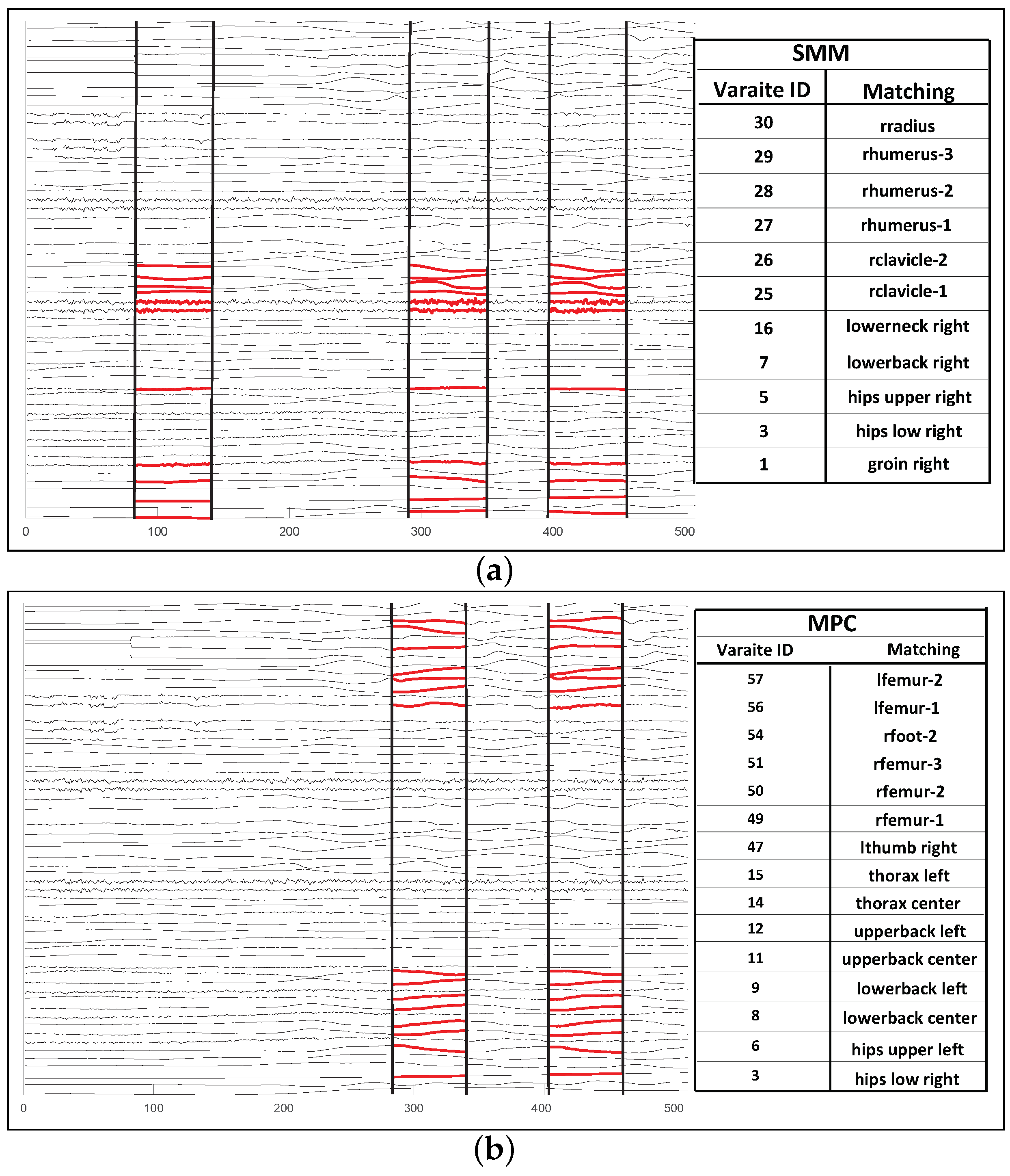
Before we present a detailed analysis of the results, we first provide a sample result to underline the key difference between the proposed SMM and the competitors. In Figure 9a, we present a multi-variate time series from the MoCap dataset [10] and the motifs identified on this series by SMM and MPC algorithms. The figure also lists the sensors involved in the recurring patterns. As we see in this figure, SMM motifs are superior:

• The motif identified by the SMM approach consists of data from sensors that are logically related in the context of action recognition. In contrast, the motif identified by the MPC approach is highly noisy; since it aims to maximize the coverage (rather than maximizing their contextual relevance), the number of sensors’ pattern includes many irrelevant sensors.
• As a side effect of this, while SMM is able to identify 3 instances of the repeated pattern, MPC is able to identify only 2 occurrences; extra sensors prevent the effective clustering of the patterns thus resulting in lower recall.

5.5. Results for the Mocap and Energy Datasets

5.5.1. Accuracy

In

Table 3. Precision, recall and F-scores for series with one motif (M1) from MoCap, for varying target overlaps (average displacement 10%).

	Precision		Recall		F-Score
Instances	SMM-s	MPC	SMM-s	MPC	SMM-s	MPC
Overlap	M1	M1	M1	M1	M1	M1
50%	0.84	0.54	0.52	0.51	0.61	0.45
75%	0.87	0.53	0.57	0.54	0.65	0.45
90%	0.92	0.51	0.64	0.49	0.71	0.43
100%	0.87	0.34	0.62	0.34	0.68	0.311

, before presenting the detailed accuracy results—from

Table 4. F-scores for time series with one motif (M1), for varying target overlaps considering multiple scales of random walk (default parameters).

	F-Score MoCap (1 Motif $\mathit{k}=$ 10, $\mathit{f}=$ 50–100%)
Instances	RW 10%		50%		RW 75%		RW 100%
Overlap	SMM-s	MPC	SMM-s	MPC	SMM-s	MPC	SMM-s	MPC
50%	0.61	0.45	0.59	0.32	0.56	0.33	0.53	0.33
75%	0.65	0.45	0.64	0.28	0.61	0.26	0.56	0.25
90%	0.71	0.43	0.69	0.22	0.66	0.22	0.62	0.21
100%	0.68	0.31	0.65	0.17	0.62	0.16	0.58	0.15
	F-Score Energy (1 Motif $\mathit{k}=$ 10, $\mathit{f}=$ 50–100%)
Instances	RW 10%		RW 50%		RW 75%		RW 100%
Overlap	SMM-s	MPC	SMM-s	MPC	SMM-s	MPC	SMM-s	MPC
50%	0.62	0.38	0.51	0.35	0.46	0.33	0.43	0.31
75%	0.52	0.27	0.41	0.22	0.37	0.21	0.35	0.19
90%	0.45	0.17	0.37	0.14	0.33	0.13	0.31	0.10
100%	0.38	0.09	0.31	0.08	0.28	0.07	0.27	0.06
	F-Score MoCap (2 Motifs $\mathit{k}=$ 10, $\mathit{f}=$ 50–100%)
Instances	RW 10%		RW 50%		RW 75%		RW 100%
Overlap	SMM-s	MPC	SMM-s	MPC	SMM-s	MPC	SMM-s	MPC
50%	0.59	0.45	0.55	0.37	0.50	0.33	0.46	0.32
75%	0.62	0.42	0.56	0.28	0.52	0.25	0.48	0.25
90%	0.67	0.32	0.61	0.24	0.57	0.22	0.51	0.23
100%	0.62	0.24	0.55	0.19	0.52	0.17	0.47	0.18
	F-Score Energy (2 Motifs $\mathit{k}=$ 10, $\mathit{f}=$ 50–100%)
Instances	RW 10%		RW 50%		RW 75%		RW 100%
Overlap	SMM-s	MPC	SMM-s	MPC	SMM-s	MPC	SMM-s	MPC
50%	0.58	0.35	0.47	0.29	0.44	0.27	0.42	0.27
75%	0.47	0.21	0.37	0.17	0.35	0.16	0.34	0.16
90%	0.43	0.12	0.35	0.1	0.32	0.08	0.31	0.08
100%	0.37	0.07	0.30	0.05	0.28	0.05	0.26	0.05
	F-Score MoCap (3 Motifs $\mathit{k}=$ 10, $\mathit{f}=$ 50–100%)
Instances	RW 10%		RW 50%		RW 75%		RW 100%
Overlap	SMM-s	MPC	SMM-s	MPC	SMM-s	MPC	SMM-s	MPC
50%	0.57	0.48	0.52	0.42	0.47	0.38	0.44	0.35
75%	0.61	0.43	0.56	0.31	0.51	0.27	0.47	0.25
90%	0.63	0.34	0.58	0.25	0.52	0.23	0.49	0.21
100%	0.56	0.23	0.51	0.20	0.47	0.19	0.43	0.18
	F-Score Energy (3 Motifs $\mathit{k}=$ 10, $\mathit{f}=$ 50–100%)
Instances	RW 10%		RW 50%		RW 75%		RW 100%
Overlap	SMM-s	MPC	SMM-s	MPC	SMM-s	MPC	SMM-s	MPC
50%	0.55	0.37	0.46	0.29	0.43	0.26	0.41	0.24
75%	0.44	0.19	0.36	0.15	0.34	0.14	0.33	0.13
90%	0.40	0.09	0.33	0.07	0.30	0.07	0.29	0.06
100%	0.34	0.05	0.29	0.04	0.27	0.03	0.25	0.03

,

Table 5. F-scores for time series with recurring patterns for varying number of recurrence counts using MoCap (default parameters, various k).

	F-Score MoCap (1 Motif $\mathit{k}=$ 5, $\mathit{f}=$ 50–100%)
Instances	RW 10%		RW 50%		RW 75%		RW 100%
Overlap	SMM-s	MPC	SMM-s	MPC	SMM-s	MPC	SMM-s	MPC
50%	0.69	0.33	0.70	0.30	0.66	0.33	0.57	0.32
75%	0.74	0.31	0.73	0.25	0.67	0.24	0.57	0.22
90%	0.75	0.27	0.74	0.19	0.68	0.20	0.57	0.17
100%	0.70	0.18	0.67	0.15	0.61	0.15	0.51	0.14
	F-Score Energy (1 Motif $\mathit{k}=$ 5, $\mathit{f}=$ 50–100%)
Instances	RW 10%		RW 50%		RW 75%		RW 100%
Overlap	SMM-s	MPC	SMM-s	MPC	SMM-s	MPC	SMM-s	MPC
50%	0.66	0.14	0.60	0.17	0.50	0.15	0.43	0.14
75%	0.52	0.10	0.45	0.11	0.37	0.09	0.32	0.09
90%	0.45	0.07	0.41	0.07	0.34	0.06	0.29	0.07
100%	0.34	0.05	0.30	0.06	0.24	0.05	0.20	0.05
	F-Score MoCap (1 Motif $\mathit{k}=$ 15, $\mathit{f}=$ 50–100%)
Instances	RW 10%		RW 50%		RW 75%		RW 100%
Overlap	SMM-s	MPC	SMM-s	MPC	SMM-s	MPC	SMM-s	MPC
50%	0.80	0.55	0.66	0.49	0.59	0.49	0.55	0.48
75%	0.60	0.56	0.51	0.48	0.47	0.43	0.45	0.40
90%	0.53	0.48	0.47	0.38	0.44	0.32	0.43	0.26
100%	0.41	0.14	0.37	0.14	0.35	0.14	0.34	0.13
	F-Score Energy (1 Motif $\mathit{k}=$ 15, $\mathit{f}=$ 50–100%)
Instances	RW 10%		RW 50%		RW 75%		RW 100%
Overlap	SMM-s	MPC	SMM-s	MPC	SMM-s	MPC	SMM-s	MPC
50%	0.62	0.29	0.57	0.30	0.50	0.31	0.41	0.28
75%	0.53	0.23	0.47	0.24	0.41	0.23	0.36	0.19
90%	0.47	0.16	0.42	0.18	0.37	0.16	0.32	0.12
100%	0.41	0.06	0.37	0.09	0.32	0.09	0.28	0.07

and

Table 6. F-scores for time series with recurring patterns that are variate-aligned (v-aligned) vs. non-variate-aligned (v-structure) from MoCap and Energy.

Instances	RW 10%		RW 50%		RW 75%		RW 100%
Overlap	SMM-s	MPC	SMM-s	MPC	SMM-s	MPC	SMM-s	MPC
	V-ALIGNED: F-Score v- MoCap (1 Motif $\mathit{k}=$ 10, $\mathit{f}=$ 50–100%)
50%	0.61	0.45	0.59	0.32	0.56	0.33	0.53	0.33
75%	0.65	0.45	0.64	0.28	0.61	0.26	0.56	0.25
90%	0.71	0.43	0.69	0.22	0.66	0.22	0.62	0.21
100%	0.68	0.31	0.65	0.17	0.62	0.16	0.58	0.15
	V-STRUCTURE: F-Score MoCap (1 Motif $\mathit{k}=$ 10, $\mathit{f}=$ 50–100%)
50%	0.46	0.25	0.42	0.24	0.38	0.23	0.34	0.24
75%	0.46	0.23	0.41	0.18	0.37	0.16	0.31	0.16
90%	0.47	0.10	0.41	0.08	0.37	0.08	0.31	0.09
100%	0.43	0.00	0.38	0.00	0.33	0.00	0.27	0.00
	V-ALIGNED: F-Score MoCap (1 Motif $\mathit{k}=$ 10, $\mathit{f}=$ 100%)
50%	0.78	0.63	0.79	0.60	0.74	0.61	0.64	0.61
75%	0.81	0.62	0.84	0.60	0.82	0.61	0.73	0.60
90%	0.79	0.58	0.83	0.58	0.79	0.60	0.71	0.57
100%	0.64	0.45	0.65	0.45	0.63	0.44	0.55	0.43
	V-STRUCTURE: F-Score MoCap (1 Motif $\mathit{k}=$ 10, $\mathit{f}=$ 100%)
50%	0.54	0.29	0.50	0.30	0.45	0.30	0.39	0.30
75%	0.52	0.27	0.47	0.27	0.41	0.26	0.38	0.25
90%	0.51	0.21	0.45	0.22	0.39	0.23	0.35	0.21
100%	0.40	0.00	0.34	0.00	0.28	0.00	0.24	0.00
	V-ALIGNED: F-Score Energy (1 Motif $\mathit{k}=$ 10, $\mathit{f}=$ 50–100%)
50%	0.62	0.38	0.51	0.35	0.46	0.33	0.43	0.31
75%	0.52	0.27	0.41	0.22	0.37	0.21	0.35	0.19
90%	0.45	0.17	0.37	0.14	0.33	0.13	0.31	0.10
100%	0.38	0.09	0.31	0.08	0.28	0.07	0.27	0.06
	V-STRUCTURE: F-Score Energy (1 Motif $\mathit{k}=$ 10, $\mathit{f}=$ 50–100%)
50%	0.51	0.15	0.42	0.16	0.32	0.13	0.29	0.11
75%	0.41	0.07	0.33	0.06	0.27	0.06	0.25	0.05
90%	0.32	0.02	0.25	0.02	0.19	0.02	0.19	0.02
100%	0.28	0.00	0.22	0.00	0.16	0.00	0.16	0.00
	V-ALIGNED: F-Score Energy (1 Motif $\mathit{k}=$ 10, $\mathit{f}=$ 100%)
50%	0.77	0.48	0.59	0.49	0.55	0.48	0.46	0.45
75%	0.58	0.47	0.47	0.43	0.45	0.40	0.40	0.34
90%	0.52	0.40	0.44	0.32	0.43	0.26	0.38	0.23
100%	0.41	0.12	0.35	0.14	0.34	0.13	0.30	0.13
	V-STRUCTURE: F-Score Energy (1 Motif $\mathit{k}=$ 10, $\mathit{f}=$ 100%)
50%	0.67	0.26	0.52	0.27	0.41	0.27	0.35	0.26
75%	0.64	0.23	0.60	0.21	0.55	0.19	0.38	0.13
90%	0.48	0.09	0.54	0.07	0.53	0.07	0.35	0.05
100%	0.48	0.00	0.54	0.00	0.53	0.00	0.35	0.00

—, we present a set of representative results, comparing accuracies for the SMM-s and MPC algorithms, on a sample scenario (one motif extracted from each series and inserted into 10 random walk time series) based on the MoCap dataset. We use the bold fonts to highlight the best results among the alternatives. As we see in this table, SMM-s leads to a significantly higher precision and overall higher accuracy values. The table also shows that SMM-based approaches are significantly more robust (to instance overlap bounds) than MPC. This means that, as we are targeting motifs that consist of more complete sub-sequences, the proposed SMM technique can provide robust accuracies, while the accuracies of MPC drop as the lower bound gets higher.

Default Scenario. We start presenting the detailed accuracy results by considering the default scenario in which we have a pattern composed of the same repeated action, or event, happening at different speeds. The results are presented in Table 4. As we can see in the table, under the default settings and under a wide range of random walk and instance overlap thresholds, SMM provides significantly higher accuracies than its competitor.

Varying Motif Instance Counts and Length Flexibilities. In Table 5, we present the results under differing motif instance counts and varying length flexibilities. Comparing the results reported in this table with the default results in Table 4, we can seen that both algorithms are similarly robust against repeating motif instance counts; on the other hand, the results indicate that SMM-s is significantly more accurate than MPC when subsequence lengths are allowed to be flexible ($f=$ 50–100%).

Varying the Degree of Variate Alignment. In this set of experiments, we relax one other constraint; motif instances can be discovered across different variates (e.g., left and right arms). Table 6 compares the accuracies for time series where the recurring patterns are variate-aligned (or v-aligned) vs. those where the motifs can appear on different (structurally compatible) subsets of variates (i.e., v-structure). As we would expect, the overall accuracy is higher when the patterns occur on the same variates (i.e., the v-structure has somewhat lower results than the default v-aligned case); but, critically, MPC performs poorly when the recurring patterns are not variate-aligned. In contrast, SMM-s is able to identify a larger number of such patterns.

Scalability against the Number of Motifs. In all the results presented so far, the time series has a single unique motif. In the next set of experiments, we (significantly) increase the number of (MoCap) motifs injected to each multi-variate series to 10. Note that the injected motifs may include common patterns that can potentially confuse the motif search algorithms.

Table 7. F-scores for time series with 10 recurring patterns that are aligned from MoCap.

	F-Score MoCap v-Structure (10 Motif $\mathit{k}=$ 10, $\mathit{f}=$ 50–100%)
Instances	RW 10%		RW 50%		RW 75%		RW 100%
Overlap	SMM-s	MPC	SMM-s	MPC	SMM-s	MPC	SMM-s	MPC
50%	0.53	0.14	0.53	0.14	0.53	0.14	0.53	0.14
75%	0.54	0.12	0.54	0.12	0.54	0.12	0.54	0.12
90%	0.55	0.07	0.55	0.08	0.55	0.08	0.55	0.08
100%	0.49	0.05	0.48	0.05	0.48	0.05	0.48	0.05

presents the results. As we can see in this table, MPC performs poorly when multiple motifs may interact on the same multi-variate series, whereas the proposed SMS algorithm is quite robust also in this respect.

5.5.2. Efficiency

We report the execution times for SMM-s and MPC algorithms, both implemented in Matlab 2015.b on Intel(R) Core(TM), i7-7700HQ CPU at 2.80 GHz, 4 cores, with 16 GB RAM. We report the execution times for the default configuration:

• SMM-s took 6.67 s for one time series (of length 2500) to locate motifs. Roughly 97% of this (6.48 s) was spent on locating salient multi-variate subsequences (SMSs) and the rest (0.19 s) was spent on identifying frequently recurring patterns.
• In contrast, MPC took 68.2 s for the same series. Roughly 57.7% of this (39.3 s) was spent on locating matching sub-sequence pairs and the rest (28.8 s) was spent on identifying frequent patterns.

Note that, in this configuration, SMM-s is 10× faster than MPC, because it limits the motif search to salient sub-sequences and it creates descriptors that are efficient to compare.

5.6. Results for the BirdSong Dataset

Finally, we report the experiment results for the Birdsong dataset [37]. As described earlier in this section, in this dataset, the contextual relationships among the variates (frequency bands) are relatively weak and we expect relatively lower benefits from contextual saliency in motif search.

Indeed, as we can see in

Table 8. F-scores for time series with recurring patterns that are not variate-aligned from BirdSong.

	F-Score BirdSong (1 Motif $\mathit{k}=$ 10, $\mathit{f}=$ 50–100%)
Instances	RW 10%		RW 50%		RW 75%		RW 100%
Overlap	SMM-s	MPC	SMM-s	MPC	SMM-s	MPC	SMM-s	MPC
50%	0.61	0.47	0.60	0.41	0.56	0.40	0.48	0.38
75%	0.58	0.49	0.57	0.40	0.55	0.40	0.47	0.36
90%	0.65	0.50	0.64	0.45	0.58	0.43	0.48	0.36
100%	0.55	0.53	0.55	0.52	0.49	0.46	0.38	0.36
	F-Score BirdSong (1 Motif $\mathit{k}=$10, $\mathit{f}=$ 100%)
Instances	RW 10%		RW 50%		RW 75%		RW 100%
Overlap	SMM-s	MPC	SMM-s	MPC	SMM-s	MPC	SMM-s	MPC
50%	0.89	0.76	0.85	0.82	0.75	0.79	0.59	0.77
75%	0.91	0.77	0.92	0.82	0.83	0.80	0.61	0.78
90%	0.85	0.77	0.83	0.82	0.68	0.80	0.49	0.79
100%	0.42	0.76	0.39	0.82	0.33	0.80	0.22	0.78

, when we seek motifs on the same variates, MPC is a better choice for identifying same length–same variate patterns. On the other hand, as we can see in

Table 9. F-scores for time series with recurring patterns that are not variate-aligned from BirdSong.

	F-Score BirdSong v-Structure (1 Motif $\mathit{k}=$ 10, $\mathit{f}=$ 50–100%)
Instances	RW 10%		RW 50%		RW 75%		RW 100%
Overlap	SMM-s	MPC	SMM-s	MPC	SMM-s	MPC	SMM-s	MPC
50%	0.48	0.23	0.48	0.25	0.45	0.27	0.38	0.24
75%	0.41	0.16	0.40	0.17	0.40	0.18	0.35	0.13
90%	0.34	0.15	0.32	0.15	0.32	0.15	0.25	0.12
100%	0.28	0.14	0.27	0.14	0.26	0.13	0.19	0.11

, when the motifs are sought in different (coherent) variate groups and present possibly different speeds (corresponding to different temporal lengths), the proposed SMS approach significantly outperforms the competitor even for this dataset.

6. Conclusions

In this paper, we propose a context-aware frequently recurring, multi-variate motif search framework for multi-variate temporal multimedia applications. The proposed salient multi-variate motif (SMM) algorithm first identifies salient multi-variate sub-sequences in the given time series and uses their locations and sizes to guide the motif search process. Motifs do occur in many multi-variate multimedia datasets:

• Visual media data: Visual media (images, videos) often contain repeated patterns that can be analyzed to classify the activity in the video, to identify real-world events, or to render the video content searchable. Sample applications include gesture detection, manufacturing and texture analysis;
• Audio media data: Audio data also often contain repeated patterns that are analyzed to classify the audio, to identify events, or to index the audio content. Sample applications include zoology and audio surveillance;
• Other sensory media data: The use of multi-variate sensory media is increasing in many smart-media applications, including healthcare, robotics, transportation and energy.

As we experimentally show in the paper, this approach enables us to control the types (e.g., variate- and length-aligned) of multi-variate motifs we search and significantly improves the quality and effectiveness of motif search. On the other side, we would like to highlight that the number of patterns considered is typical in the motif search literature, as, in many applications, one searches for a few dominant patterns in the input media. However, we would also like to highlight that, as we can see in Table 1, Table 2 and Table 3 in the paper, independent of the number of motifs, the proposed SMM is more accurate than the state-of-the-art competitor, MPC. As reported in the paper, SMM is also much faster than MPC.

References

- Mei, T.; Rui, Y.; Li, S.; Tian, Q. Multimedia search reranking: A literature survey. ACM Comput. Surv. (CSUR) 2014, 46, 38. [Google Scholar]
- Yang, X.; Zhang, C.; Tian, Y. Recognizing actions using depth motion maps-based histograms of oriented gradients. In Proceedings of the 20th ACM International Conference on Multimedia, Nara, Japan, 29 October–2 November 2012; pp. 1057–1060. [Google Scholar]
- Weinland, D.; Ronfard, R.; Boyer, E. A survey of vision-based methods for action representation, segmentation and recognition. Comput. Vis. Image Underst. 2011, 115, 224–241. [Google Scholar]
- Scovanner, P.; Ali, S.; Shah, M. A 3-dimensional sift descriptor and its application to action recognition. In Proceedings of the 15th ACM International Conference on Multimedia, Augsburg, Germany, 25–29 September 2007; pp. 357–360. [Google Scholar]
- Torkamani, S.; Lohweg, V. Survey on time series motif discovery. Wiley Interdiscip. Rev. Data Min. Knowl. Discov. 2017, 7, e1199. [Google Scholar]
- Tanaka, Y.; Iwamoto, K.; Uehara, K. Discovery of time-series motif from multi-dimensional data based on MDL principle. Mach. Learn. 2005, 58, 269–300. [Google Scholar]
- Balasubramanian, A.; Wang, J.; Prabhakaran, B. Discovering Multidimensional Motifs in Physiological Signals for Personalized Healthcare. IEEE J. Sel. Top. Signal Process. 2016, 10, 832–841. [Google Scholar] [CrossRef]
- Balasubramanian, A.; Prabhakaran, B. Flexible exploration and visualization of motifs in biomedical sensor data. In Proceedings of the Workshop on Data Mining for Healthcare (DMH), in Conjunction with ACM KDD, Chicago, IL, USA, 11 August 2013. [Google Scholar]
- Yeh, C.C.M.; Kavantzas, N.; Keogh, E. Matrix Profile VI: Meaningful Multidimensional Motif Discovery. In Proceedings of the 2017 IEEE International Conference on Data Mining (ICDM), New Orleans, LA, USA, 18–21 November 2017; pp. 565–574. [Google Scholar] [CrossRef]
- Lab, C.G. Motion Capture Database. 2018. Available online: http://mocap.cs.cmu.edu/ (accessed on 10 October 2021).
- Buhler, J.; Tompa, M. Finding motifs using random projections. In Proceedings of the Fifth Annual International Conference on Computational Biology, ACM, RECOMB ’01, Montreal, QC, Canada, 22–25 April 2001; pp. 69–76. [Google Scholar]
- Patel, P.; Keogh, E.; Lin, J.; Lonardi, S. Mining Motifs in Massive Time Series Databases. Proceedings of IEEE International Conference on Data Mining (ICDM’02), Maebashi City, Japan, 9–12 December 2002; pp. 370–377. [Google Scholar]
- Keogh, E.; Lin, J.; Truppel, W. Clustering of Time Series Subsequences is Meaningless: Implications for Previous and Future Research. In Proceedings of the Third IEEE International Conference on Data Mining, ICDM ’03, Melbourne, FL, USA, 19–22 November 2003; pp. 115–125. [Google Scholar]
- Zhang, X.; Wu, J.; Yang, X.; Ou, H.; Lv, T. A novel pattern extraction method for time series classification. Optim. Eng. 2009, 10, 253–271. [Google Scholar]
- Esling, P.; Agon, C. Time-series data mining. ACM Comput. Surv. 2012, 45, 1–34. [Google Scholar] [CrossRef] [Green Version]
- Tang, H.; Liao, S.S. Discovering original motifs with different lengths from time series. Know.-Based Syst. 2008, 21, 666–671. [Google Scholar] [CrossRef]
- Ferreira, P.G.; Azevedo, P.J.; Silva, C.G.; Brito, R.M.M. Mining Approximate Motifs in Time Series. In Discovery Science; Todorovski, L., Lavrac, N., Jantke, K., Eds.; Lecture Notes in Computer Science; Springer: Berlin/Heidelberg, Germany, 2006; Volume 4265, pp. 89–101. [Google Scholar]
- Lin, J.; Keogh, E.; Lonardi, S.; Chiu, B. A symbolic representation of time series, with implications for streaming algorithms. In Proceedings of the 8th ACM SIGMOD Workshop on Research Issues in Data Mining and Knowledge Discovery, San Diego, CA, USA, 13 June 2003; pp. 2–11. [Google Scholar]
- Chiu, B.; Keogh, E.; Lonardi, S. Probabilistic discovery of time series motifs. In Proceedings of the Ninth ACM SIGKDD International Conference on Knowledge Discovery and Data Mining, KDD ’03, Washington, DC, USA, 24–27 August 2003; pp. 493–498. [Google Scholar]
- Yankov, D.; Keogh, E.; Medina, J.; Chiu, B.; Zordan, V. Detecting time series motifs under uniform scaling. In Proceedings of the 13th ACM SIGKDD International Conference on Knowledge Discovery and Data Mining, KDD ’07, San Jose, CA, USA, 12–15 August 2007; pp. 844–853. [Google Scholar]
- Castro, N.; Azevedo, P. Multiresolution Motif Discovery in Time Series. In Proceedings of the SIAM International Conference on Data Mining, Columbus, OH, USA, 29 April–1 May 2010; pp. 665–676. [Google Scholar]
- Mueen, A.; Keogh, E.J.; Zhu, Q.; Cash, S.; Westover, M.B. Exact Discovery of Time Series Motifs. In Proceedings of the SIAM International Conference on Data Mining, Sparks, NV, USA, 30 April–2 May 2009; pp. 473–484. [Google Scholar]
- Lam, H.T.; Calders, T.; Pham, N. Online Discovery of Top-k Similar Motifs in Time Series Data. In Proceedings of the SIAM International Conference on Data Mining, Mesa, AZ, USA, 28–30 April 2011; pp. 1004–1015. [Google Scholar]
- Mohammad, Y.; Nishida, T. Constrained Motif Discovery in Time Series. New Gener. Comput. 2009, 27, 319–346. [Google Scholar] [CrossRef]
- Yeh, C.C.M.; Zhu, Y.; Ulanova, L.; Begum, N.; Ding, Y.; Dau, H.A.; Silva, D.F.; Mueen, A.; Keogh, E. Matrix Profile I: All Pairs Similarity Joins for Time Series: A Unifying View That Includes Motifs, Discords and Shapelets. In Proceedings of the 2016 IEEE 16th International Conference on Data Mining (ICDM), Barcelona, Spain, 12–15 December 2016; pp. 1317–1322. [Google Scholar] [CrossRef]
- Grünwald, P.D.; Myung, I.J.; Pitt, M.A. Advances in Minimum Description Length: Theory and Applications; MIT Press: Cambridge, MA, USA, 2005. [Google Scholar]
- Vahdatpour, A.; Amini, N.; Sarrafzadeh, M. Toward Unsupervised Activity Discovery Using Multi-Dimensional Motif Detection in Time Series. In Proceedings of the 21st International Joint Conference on Artificial Intelligence, Pasadena, CA, USA, 11–17 July 2009; Volume 9, pp. 1261–1266. [Google Scholar]
- Minnen, D.; Isbell, C.; Essa, I.; Starner, T. Detecting subdimensional motifs: An efficient algorithm for generalized multivariate pattern discovery. In Proceedings of the Seventh IEEE International Conference on Data Mining (ICDM 2007), Omaha, NE, USA, 28–31 October 2007; pp. 601–606. [Google Scholar]
- Minnen, D.; Starner, T.; Essa, I.A.; Isbell, C.L., Jr. Improving Activity Discovery with Automatic Neighborhood Estimation. In Proceedings of the 20th International Joint Conference on Artificial Intelligence, Hyderabad, India, 6–12 January 2007; Volume 7, pp. 2814–2819. [Google Scholar]
- Minnen, D.; Isbell, C.L.; Essa, I.; Starner, T. Discovering multivariate motifs using subsequence density estimation and greedy mixture learning. In Proceedings of the National Conference on Artificial Intelligence, Vancouver, BC, Canada, 22–26 July 2007; AAAI Press: Menlo Park, CA, USA; Cambridge, MA, USA; London, UK; MIT Press: Cambridge, MA, USA, 2007; Volume 22, p. 615. [Google Scholar]
- Minnen, D.; Starner, T.; Essa, I.; Isbell, C. Discovering characteristic actions from on-body sensor data. In Proceedings of the 10th IEEE International Symposium on Wearable Computers, Montreux, Switzerland, 11–14 October 2006; pp. 11–18. [Google Scholar]
- Lowe, D.G. Object Recognition from Local Scale-Invariant Features. In Proceedings of the International Conference on Computer Vision, ICCV ’99, Corfu, Greece, 20–25 September 1999. [Google Scholar]
- Lowe, D.G. Distinctive Image Features from Scale-Invariant Keypoints. Int. J. Comput. Vis. 2004, 60, 91–110. [Google Scholar]
- Garg, Y.; Poccia, S.R. On the Effectiveness of Distance Measures for Similarity Search in Multi-Variate Sensory Data: Effectiveness of Distance Measures for Similarity Search. In Proceedings of the 2017 ACM on International Conference on Multimedia Retrieval, ICMR 2017, Bucharest, Romania, 6–9 June 2017; pp. 489–493. [Google Scholar] [CrossRef]
- Ester, M.; Kriegel, H.P.; Sander, J.; Xu, X. A Density-based Algorithm for Discovering Clusters in Large Spatial Databases with Noise. In Proceedings of the Second International Conference on Knowledge Discovery and Data Mining, KDD’96, Portland, OR, USA, 2–4 August 1996; AAAI Press: Palo Alto, CA, USA, 1996; pp. 226–231. [Google Scholar]
- Energy Data for a Building with 27 Zones. Available online: https://drive.google.com/file/d/1qeL6u5Ik5hMSYDeVFp4WpweHQxQ_JZRH/view?usp=sharing (accessed on 20 May 2021).
- BirdSong (13 MFCC Coefficients for 154 Bird Calls). Available online: http://www.xeno-canto.org/explore/taxonomy (accessed on 20 May 2021).
Figure 1.
In this motion capture snippet (from MoCap [10]), the repeated pattern (dribble action) is focused on the sensors corresponding to the right arm; note that not all dribble actions were performed at the same speed.
Figure 2.
In this motion snippet (from MoCap [10]), the repeated pattern (climbing action) occurs on different sets of variates—alternately on sensors on the right and left arms.
Figure 3.
(a) Motion capture involves capturing the positions of multiple sensors placed on the human body (the positioning of the sensors are taken from [10]); (b) consequently, the resulting multi-variate time series needs to be interpreted within the context of the metadata describing the relationships among the sensor variates.
Figure 4.
Local salience of a subsequence implies that it is well defined in its immediate neighborhood; is different from a larger subsequence centered around the same time point.
Figure 5.
Overview of the SMM for contextually salient multi-variate motif discovery.
Figure 6.
Scale-space construction through iterative smoothing in time and variates (details in Figure 7).
Figure 7.
Increasing the temporal and variate smoothing rate reduces the details across (by taking into account the available metadata). (a) Original series; (b) Smoothed (and reduced) series.
Figure 8.
Heatmap visualization of sample time series: each row corresponds to a different variate (best viewed in color). (a) MOCAP sample. (b) Building energy sample. (c) BirdSong sample.
Figure 9.
Sample motifs identified by the proposed SMM approach and a competitor (MPC [25]). The motifs extracted by SMM are contextually meaningful, whereas MPC’s motifs (obtained without considering the metadata associated with the time series) are noisy. (a) Sample SMM motif—note that the repeating pattern is detected on sensors at the same (right) side of the body. (b) Corresponding motif identified by a competitor—some sensors included in the motif include those that are irrelevant to the action; the motif also misses one recurring instance.