Towards Robust Object Detection in Floor Plan Images: A Data Augmentation Approach

Abstract

Object detection is one of the most critical tasks in the field of Computer vision. This task comprises identifying and localizing an object in the image. Architectural floor plans represent the layout of buildings and apartments. The floor plans consist of walls, windows, stairs, and other furniture objects. While recognizing floor plan objects is straightforward for humans, automatically processing floor plans and recognizing objects is challenging. In this work, we investigate the performance of the recently introduced Cascade Mask R-CNN network to solve object detection in floor plan images. Furthermore, we experimentally establish that deformable convolution works better than conventional convolutions in the proposed framework. Prior datasets for object detection in floor plan images are either publicly unavailable or contain few samples. We introduce SFPI, a novel synthetic floor plan dataset consisting of 10,000 images to address this issue. Our proposed method conveniently exceeds the previous state-of-the-art results on the SESYD dataset with an mAP of 98.1%. Moreover, it sets impressive baseline results on our novel SFPI dataset with an mAP of 99.8%. We believe that introducing the modern dataset enables the researcher to enhance the research in this domain.

1. Introduction

Object detection is one of the most elementary and essential tasks in the field of computer vision. In object detection, we deal with the identification and localization of objects present in the image or video [1,2]. Architectural floor plans contain both structural and semantic information, e.g., room size, type, location of doors, walls, and furniture [3]. Object detection in floor plan images is an integral step in the field of floor plan analysis. Due to the intricate nature of floor plan images, it is challenging to interpret their semantic meaning. Moreover, there is an inherent relationship between the room types and furniture objects, walls, and windows. For instance, the kitchen only contains a limited set of furniture objects. Floor plan images have several applications, such as CAD model generation [4], 3D model creation for interactive walkthroughs [5] or similarity search [6]. We present a couple of floor plan images with different information to understand the semantics of floor plan layouts. Figure 1 illustrates information about different rooms and their sizes in the floor plan. In Figure 1, the top left room is marked as a kitchen where the dining table is present. The room next to this is identified as the living room, where various sofa objects are present. Similarly, additional rooms are identified with different furniture objects. This type of floor plan is useful for interactive furniture fitting [5].

In Figure 2, the top left room contains a coffee table and a sink, whereas the bottom left room contains a chair and sofa. Similarly, the remaining rooms have other furniture objects. Contrarily to Figure 1, apart from the localization of furniture object, no other information is available in Figure 2. Identifying the furniture objects present in a floor plan image enables us to distinguish the type of room, i.e., kitchen, living room, and so on. We also have a few common elements like furniture objects, walls, windows, and doors. These are some common artifacts that exist in every floor plan image [3]. Identifying the floor plan objects is the preliminary step towards the analysis of the floor plan images. Our main work focuses on this preliminary step to detect the furniture objects, doors, and windows in the floor plan images. Detecting these objects is difficult due to the variety of floor plan layouts available. Furthermore, individual furniture objects are not always similar, i.e., we can have multiple types of chairs and windows in a floor plan image. One of the critical ideas of our research is to create an end-to-end trainable framework that can handle different varieties of furniture objects and generalize well. In order to develop a robust learning-based model, we need a large-scale dataset that should include different varieties of floor plan layouts and furniture objects.

There exist only a few publicly available datasets for floor plan images [4,7,8]. Besides fewer samples, less variation in floor plan layouts and furniture objects are also a concern for the floor plan datasets. It is challenging to train deep detectors using the currently available floor plan datasets. We have created our custom dataset to fill this gap, containing 10,000 images with various floor plans and furniture objects. This dataset will be available publicly for further enhancement and experiments. Figure 3 represents a floor plan where all furniture objects are masked and highlighted based on the bounding box information and corresponding class labels that are present in the ground truth of the SESYD dataset [3].

Although object detection algorithms have been applied before on floor plan images [9,10,11], most of them employ Faster R-CNN [12], YOLO [13] or other pattern matching algorithms [14]. Contrarily, we propose a framework that operates Cascaded Mask R-CNN [15] for object detection in floor plan images. We employ both conventional convolution and deformable convolutional networks (DCN) [16] on the backbone network and compare the performance, comparing them with baseline methods. This paper presents an end-to-end approach for object detection in floor plan images. The main contributions of this paper are as follows:

• We present an end-to-end trainable framework that works on Cascade Mask R-CNN [15] with conventional and deformable [16] convolutional backbone network to detect various objects in floor plan images.
• We publish SFPI (Synthetic Floor Plan Images), a novel floor plan dataset comprising 10,000 images. This dataset includes ten different floor plan layouts and 16 different classes of furniture objects. The dataset is available here https://cloud.dfki.de/owncloud/index.php/s/mkg5HBBntRbNo8X (accessed on 5 October 2021).
• Our proposed method accomplishes state-of-the-art results on the publicly available SESYD dataset [3] and establishes impressive baseline results for the newly proposed dataset.

The rest of the paper is organized as follows. In Section 2, we describe the literature survey in the field of floor plan image object detection. Section 3 discusses the architecture of our proposed model. We discuss the architecture of Cascade Mask R-CNN [15], our backbone network [17], and deformable convolutions [16]. In Section 4, we talk about existing datasets and problems related to these datasets. Then, we analyze the peculiarities of our custom floor plan dataset. In Section 5, we explain our implementation configurations and different experiments. We also evaluate the results of these experiments and compare them with the previous state-of-the-art results. Our conclusions and pointers for future work are explained in Section 6.

2. Related Work

Recent advancements in deep learning methodologies [14,17,18,19,20,21] have significantly affected the computer vision approaches like object detection [12,15]. We have quite a few detectors available as per the orientation of specific tasks. In one of the recent works [10], the authors extract structural information from floor plan images to estimate the size of the rooms for interactive furniture fitting. In order to achieve this, first wall segmentation is carried out using a fully convolutional neural network; afterward, they detect objects using a Faster R-CNN, and finally, they perform optical character recognition to detect dimensions of a different room. Faster R-CNN was the main detector used for object detection in floor plan images. In [22], the authors address the floor plans with different notations. They use segmentation of walls, doors, and windows to understand the floor plan images better. They tested on publicly available dataset CVC-FP [7], which contains four different floor plans. It is good to have different floor plans in our dataset as this creates a variety of images and improves the performance of our model.

In [23], the authors presented a table detection framework from scanned document images based on Cascade Mask R-CNN [15]. The authors used recursive feature pyramid network and switchable atrous convolution to obtain a comparable result without relying on pre-and post-processing methods and heavier backbone networks. The presented work achieves state-of-the-art results on publicly available table detection datasets. In another work [24], the authors used Cascade Mask R-CNN [15] for detecting formulas in scanned document images. The authors used dual backbone of ResNeXt-101 [17] with deformable convolution to achieve higher detection accuracy.

In [25], the authors proposed a powerful backbone named composite backbone network. This backbone assembles multiple identical backbones by composite connections between the parallel stages of the adjacent backbones. It feeds the output of the previous backbone as input to the succeeding backbone. This composite backbone combined Cascade Mask R-CNN [15] was able to achieve results better than state-of-the-art for object detection in dataset COCO [26]. This shows that Cascade Mask R-CNN [15] is amongst one of the best performing networks in object detection. In another work [27], the author used different detectors to improve robotic vision and probability object detection in real-life scenarios. Gamma correction and data augmentation were applied to deal with the large brightness variation in day and night. Moreover, a virtual dataset was used to increase the richness of surrounding conditions. From the results, it is evident that Cascade Mask R-CNN [15] performs better than its predecessors.

In [28], the authors presented an approach to detect aero-engine blade damage. Aero-engine blades affect the performance and safety of an aircraft. It is important to detect and identify the damages to these blades intelligently. The authors used Cascade Mask R-CNN [15] and improved it further in order to accomplish an accuracy rate of 98.81%. Further comparison with other detectors was also part of their study. In [29], the authors proposed a framework for high-quality segmentation and object detection in remote sensing imagery. Cascade Mask R-CNN [15] was used with max-batch soft IoU for object identification and instance segmentation. The authors employed IoU as a loss function to solve the mismatch issue between the loss function and the evaluation metric. In [30], the authors presented a network to understand assembly instruction like furniture assembly. There are several components in furniture assembly instructions, such as furniture parts, mechanical connectors, symbols, and numbers. The authors used Cascade Mask R-CNN [15] and developed a context-aware data augmentations scheme for speech bubble segmentation that combines image cuts by considering the context of assembly instructions.

In [31], the author attempted to parse floor plan images using deep learning detectors. The author used Cascade Mask R-CNN [15] to extract the information from a floor plan image and used keypoint-CNN in segmentation to find precise locations of corners, which is further combined in the post-processing step to give the resulting segmentation. In [32], the authors attempt to synthesize a textual description from a floor plan image. This is another good application for floor plan analysis. This can help visually impaired people to imagine the interiors of the house, and it is also helpful for potential buyers of the house who are located far. The authors detect walls by performing morphological closure on the input floor plan image; doors are detected using the scale-invariant feature, and then connected components are identified using the flood fill technique. Once this information was available, then text processing was applied.

In another work presented by Zeng et al. [33], the authors proposed a method for floor plan recognition, with a focus on recognizing diverse floor plan elements, e.g., walls, doors, rooms, and furniture. The authors used a shared VGG [34] encoder to extract features from the input floor plan images. It detects the room-boundary for walls, windows, and doors. It also detects the room type based on the elements in the room. The number of furniture items used to identify the room type is less. However, the authors get good results in detecting walls, windows, and doors.

In one of the recent works on floor plans, the authors [11] created a framework for floor plan recognition and reconstruction. The authors used text detection as well as symbol detection to identify room types. Symbol detection is identifying different furniture objects available in the room and, based on it, determining the type of the room. The authors use YOLO4 [35] as a base network for identifying symbols in different rooms. This is also supported by the information from the text detection. Once all the required information is present, vectorization is performed on the floor plan images to reconstruct a new floor plan image.

In [10], the authors presented a method to detect the elements in the floor plan images, wall, and windows, as well as to determine the text from floor plan images. The authors used a fully convolutional network (FCN) and optical character recognition (OCR) technique. Experiments were performed on CVC-FP [7] and self-collected datasets. The experiments performed on the datasets were: wall segmentation, object detection, and text recognition. Although promising wall segmentation was reported, the number of testing samples to evaluate the object detection and text recognition performance was relatively low.

Another work for object detection in floor plan images was done by Ziran et al. [9], where the authors analyzed different available datasets in the floor plan domain and created their own custom datasets. They used Faster R-CNN [12] with ResNet-101 [19] as backbone for detecting furniture objects in the floor plan images. The custom dataset used in this experiment has fewer furniture class objects and fewer samples. Thus, the work does not provide conclusive empirical evidence to verify the effectiveness of the proposed method. From the results, we can identify that the network, which was pre-trained on COCO [26] dataset, performs well.

Based on all these works, we can identify that furniture object detection is the preliminary step in processing floor plan images irrespective of the application. Whether we want to generate some text-based synthesis for floor plan images or we want to reconstruct the floor plan images, we must identify the objects available in different rooms of the floor plan and identify doors and windows correctly. Our work mainly focuses on identifying the furniture objects, windows, and walls in floor plan images, creating a base for all the applications mentioned above.

3. Method

The presented approach is based on Cascade Mask R-CNN [15] equipped with backbone ResNeXt-101 [17]. We have implemented this model with conventional convolutional networks (CNN) as well as deformable convolutional networks (DCN) [16]. The Figure illustrates the complete pipeline of our proposed framework. In this section, we dive deep into the individual components of our proposed method.

3.1. Cascade Mask R-CNN

Cascade Mask R-CNN [15] was introduced by Cai and Vasconcelos, which is a multi-stage extension of Faster R-CNN [12]. Cascade Mask R-CNN [15] has a similar architecture as Faster R-CNN, but along with an additional segmentation branch, which is denoted as ’S’ in Figure 4, for creating masks of the detected objects. Figure 4 shows that the input image is passed through the ResNeXt-101 [17] backbone, which is explained in Section 3.2. The backbone extracts the spatial features from the images and generates feature maps. The possible candidate regions where furniture objects might be present in the images are estimated by the region proposal network (RPN) head. These proposals are passed through the ROI pooling layer. The network head takes ROI features as input and makes two predictions: classification score (C) and bounding box regression (B). All three bounding box modules perform classification and regression. The output of one bounding box head is used as training input for the next head. These deeper detector stages are more selective against false positives even at higher IoU thresholds. Each regressor is optimized for the bounding box distribution generated by the previous regressor rather than the initial distribution. We get a bounding box of higher IoU thresholds when we train the bounding box regressor for a certain IoU threshold. We get refined bounding boxes and classification scores from B3, and the segmentation head predicts the mask that contributes to the loss function to optimize the training further.

3.2. Backbone Network

We employ ResNeXt-101 [17] as backbone for our experiment. ResNeXt-101 [17] uses cardinality features as compared to its previous version, ResNets [19]. In ResNeXt, a layer is shown as the number of in channels, filter size, and the number of out channels. This network stacks residual blocks. These blocks are subject to two simple rules: (i) if the same size spatial maps are produced, the blocks share the same hyperparameters, and (ii) every time when the spatial map is downsampled by a factor of 2, the width of the blocks is multiplied by a factor of 2. This ensures consistency in computation complexity in terms of FLOPs. In an artificial neural network, neurons perform inner product, which can be thought of as a form of aggregating transformation:

$$\sum _{i=1}^D{w}_i{x}_i$$

(1)

where x is the D-channel input vector to neuron and $w_i$ is a filter’s weight for the i-th channel. This has been updated in the ResNeXt [17] architecture with a more generic function, which can be a network in itself. Aggregated transformations are represented as:

$$f\left(x\right)=\sum _{i=1}^C{\tau }_i\left(x\right)$$

(2)

where ${\tau }_i\left(x\right)$ can be an arbitrary function that projects x into an (optionally lower dimension) embedding and then transforms it. The C is the size of transformations to be aggregated, referred to as cardinality. In Equation (2), C looks the same as D in Equation (1), but C needs not equal D and can be an arbitrary number. This aggregated transformation serves as the residual function:

$$y=x+\sum _{i=1}^C{\tau }_i\left(x\right)$$

(3)

where y is the output which is then further propagated to the region proposal network of our Cascade Mask R-CNN as explained in Figure 4.

3.3. Deformable Convolution

Apart from conventional convolution available in ResNeXt-101 [17], we incorporate deformable convolution filters [16]. A convolutional neural network uses local connections to extract spatial information effectively and shared weights. Convolutional layers at higher levels identify complete objects, whereas layers at the bottom look for fine features like edges and corners of the gradients. In standard 2D convolution, we apply 2D filter/kernels over the input at the fixed receptive field and spatial locations to generate the output feature map. The output feature map is generated by a convolution operation between kernel w and the input x, which can be formulated as $y=w\times x$ and every element in feature map y can be calculated as:

$$y\left(p_0\right)=\sum _{p_i\in C}w\left(p_i\right).x(p_0+p_i)$$

(4)

where $p_0$ is the center location of the sample in the input, and $p_i$ enumerates the points in the collection of sampling points. Because different locations in the input feature maps may correspond to objects with different scales or deformation, adaptive determination of receptive field sizes is desirable for certain tasks.

Deformable convolution has a learnable shape to adapt to changes in features; this is explained in Figure 5. Deformable convolution makes the sampling matrix learnable, allowing the shape of the kernel to adapt to the unknown complex transformations in the input. Instead of using the fixed sampling matrix with fixed offsets, as in standard convolution, the deformable convolution learns the sampling matrix with location offsets. The offsets are learned from the preceding feature maps via additional convolutional layers. Thus, the deformation is conditioned on the input features in a local, dense, and adaptive manner. To put this into the equation, in deformable convolution, the regular sampling matrix C is augmented with offsets $▵p_i|n=1,\dots ,n$, where $N=\left|C\right|$. Equation (4) becomes:

$$y\left(p_0\right)=\sum _{p_i\in C}w\left(p_i\right).x(p_0+p_i+▵p_1)$$

(5)

where $p_0$ is the center location of the sample in the input, and $p_1$ enumerates the points in the collection C of sampling/offset points. Now the sampling is on the irregular and offsets locations $p_i+▵p_i$.

4. Dataset

The prior literature on floor plan images reflects that there is a scarcity of datasets in this area. SESYD [3], CVC-FP [7], and ROBIN [8] are the 3 most widely used publicly available datasets in this area. SESYD [3] contains synthetic floor plan images with furniture objects placed in different rooms randomly. It has 10-floor plan layouts and, in total, contains 1000 images. Although this idea is fascinating to put furniture objects randomly, the overall number of images is less. It has 16 different furniture classes.

In the CVC-FP [7] dataset, we only have 122-floor plan images. These floor plan images are distributed amongst four different floor plan layouts. Overall, the total number of furniture classes is also less and limited to 4 classes. This dataset is not suitable for the training of the deep neural network [20].

In the ROBIN [8] dataset, we have different hand-drawn as well as synthetically generated images. In this dataset also, we have only a limited number of images 510. Floor plan layouts and furniture object classes are also limited.

To train a deep detector, we need a dataset with sufficient images and variety in the floor plan layouts to generalize the network for realistic images. Moreover, the number of furniture classes should be large enough to identify different varieties of furniture objects. To address this, we create our custom dataset, which is based on the SESYD [3] dataset. We named our custom dataset SFPI (Synthetic Floor Plan Images). From this point onward, we will describe our custom dataset with the name SFPI.

In Figure 6, we have a sample floor plan image from the SESYD [3] dataset. It has various furniture objects present in different rooms. It is visible from the image that the scale of different furniture classes among them is almost the same and rarely varies; we observed this behavior in the full dataset as well. It is also noticeable that the orientation of different furniture objects also does not vary a lot. Moreover, we observe that few furniture objects are available in specific rooms, which is good if we want to identify room types but not for our purpose of detecting furniture objects. We want to generalize the model so that it can identify the objects available in any room. Keeping all these shortcomings of the SESYD [3] dataset in mind, we propose our dataset SFPI.

4.1. Dataset Creation

To generate the custom dataset SFPI, we took all floor plan layouts of SESYD [3] as the base and implanted the furniture objects to create different floor plan images. To overcome the shortcomings of SESYD [3], we take care of furniture object augmentations. The first augmentation we apply is rotation; we assign rotation randomly on furniture class objects. In this way, some objects will undergo rotation, and some will be the same as the original model. We use random angle choices between [0, 30, 45, 60, 75, 90, 120, 150, 180, 210, 250, 270, 300, 330] degrees and rotate the image from its center. Figure 7 depicts the example of this augmentation; Sofa and Tub furniture class objects have different orientations based on randomly selected angels. Another augmentation choice we employ is scaling; this is an important step to ensure that the model generalizes well to identify natural furniture objects. We enforce scaling randomly to have both scaled and non-scaled furniture class objects in the same image. For scaling, we use a random resize factor between [40, 60, 75, 85, 100, 130, 145, 160, 185, 200] and scale the objects using this. We use the inter-are option for interpolation while resizing the objects. While resizing, we make sure to keep the original aspect ratio of the objects intact. In Figure 7, we have different scaling for bed and sofa objects of respective furniture classes.

4.2. SFPI Statistics

Our SFPI dataset has ten different floor plan layouts and 16 different furniture classes, including armchair, bed, door1, door2, sink1, sink2, sink3, sink4, sofa1, sofa2, table1, table2, table3, tub, window1, window2. We also have multiple variants of the same class type to cover different varieties of furniture objects. It helps in generalizing the model for a more realistic output. We have created 10,000 images. Each floor plan layout has 1000 images. Overall, we have 316,160 objects of different furniture classes across these 10,000 images. Figure 8 illustrates the furniture class distribution of our SFPI dataset.

Figure 8 depicts that doors and windows classes have the highest number of objects in the dataset. This is natural because, in each floor plan, the number of doors and windows is always higher than other individual furniture objects. We can identify that, at a minimum, we have around 5000 representations of any class in our SFPI dataset.

Table 1. Statistical comparison between SESYD [3] and the proposed SFPI datasets. The distribution of images to train our base model on both datasets.

Dataset	Objects	Train	Val	Test
SESYD [3]	20,670	700	150	150
SFPI	316,160	7000	1500	1500

explains the image distribution we use for training and testing our model. While working on the original SESYD [3] dataset, we take 700 images for training and 150 images for both validation and testing. A total of 20,670 different furniture objects are available in these 1000 images. While working on our custom dataset SFPI, we use the same 70-30 rule for splitting. We used 7000 images for training and 1500 images for both validation and testing. Now, as the number of images is increased, we have more furniture objects available. We performed multiple experiments using these two datasets; all information related to these experiments is available in Section 5.

5. Experimental Results

5.1. Implementation Details

We implement the proposed method using PyTorch and MMDetection’s object detection pipeline [36]. Our backbone ResNeXt-101 [17] is pre-trained on MS-COCO dataset [26]. Using this pre-trained feature extraction backbone helps our architecture to adapt from the domain of natural scenes to floor plan images. We scale our input floor plan images to $1333\times 800$, keeping the original aspect ratio. For efficient execution [21] on our setup we use a batch size of one to train our network. The initial learning rate for training is 0.0025. We train the network for 12 iterations on our SFPI dataset. The IoU threshold value for cascaded bounding boxes is set to [0.5, 0.6, 0.7]. We use three different anchor rations of [0.5, 1.0, 2.0] and strides of [4, 8, 16, 32, 64] and with only one anchor scale of [8] since FPN [37] itself performs multiscale detection because of its top-down architecture. We use Cross-Entropy loss for calculating network losses. Furthermore, we apply both traditional convolution and DCN [16] backbone networks for different experiments. However, overall experiment settings for both are the same, apart from the choices of datasets. We trained on GeForce GTX 1080 GPU [38] in coordination with 4 CPUs and with 25 GB memory.

5.2. Evaluation Criteria

As this is an object detection problem, we use the detection evaluation matrix of COCO [26]. The employed evaluation metrics are explained as follows:

5.2.1. Intersection over Union

Intersection over Union (IoU) [39] is defined as the area of the intersection divided by the area of the union of a predicted bounding box $\left(B_p\right)$ and a ground-truth box $\left(B_{gt}\right)$:

$$IoU=\frac{area(B_p\cap B_{gt})}{area(B_p\cup B_{gt})}$$

(6)

IoU is used as a criterion that determines whether detection is a true positive or a false positive.

5.2.2. Average Precision

Average precision [40] is based on the precision–recall curve. It is useful when we are comparing different detectors and the precision–recall curves intersect with each other. AP can be defined as the area under the interpolated precision-recall curve, which can be calculated using the following formula:

$$AP=\sum _{i=1}^{n-1}(r_{i+1}-r_i)p_{interp}\left(r_{i+1}\right)$$

(7)

where $r_1,r_2,\dots ,r_n$ are the recall levels at which the precision is first interpolated.

5.2.3. mAP

The calculation of AP only involves one class. However, in object detection, there are usually $K>1$ classes. Mean average precision (mAP) [26] is defined as the mean of AP across all K classes:

$$mAP=\frac{{\sum }_{i=1}^{K}A{P}_i}{K}$$

(8)

5.2.4. Average Recall

Average recall (AR) [40] like AP can be used to compare detector performance. AR is the recall averaged over all $IoU\in [0.5,1.0]$ and can be computed as two times the area under the recall-IoU curve:

$$AR=2{\int }_{0.5}^{1}recall\left(o\right)do$$

(9)

where o is IoU and $recall\left(o\right)$ is the corresponding recall. For the COCO dataset, AR metric is calculated on a per-class basis, like AP.

5.2.5. Mean Average Recall (mAR)

Mean average recall [26] is defined as the mean of AR across all K classes:

$$mAR=\frac{{\sum }_{i=1}^{K}A{R}_i}{K}$$

(10)

5.3. Results and Discussion

We validate our proposed framework on both the SESYD [3] and the SFPI dataset to demonstrate its effectiveness. In this section, we will discuss the quantitative and qualitative performance of our approach. We will discuss the strength and weaknesses of our model. Furthermore, we will compare our results with current state-of-the-art methods.

5.3.1. SESYD

For this dataset, we use a split of 70-30 as mentioned in Section 4. We use 700 random images out of 1000 for training the network, and from the remaining images, 150 for test and 150 for validation. We follow the evaluation protocol of COCO [26] performance metrics.

All models mentioned in

Table 2. Quantitative analysis of our model with existing state-of-the-art methods.

		Mean Average Precision (mAP)		Mean Average Recall (mAR)
Model_Dataset	Objects	Val	Test	Val	Test
Our_SESYD	20,670	0.981	0.982	0.986	0.987
Ziran et al. [9]—d1	1111	-	0.31	-	0.60
Ziran et al. [9]—d2	1111	-	0.39	-	0.69

are pre-trained on COCO [26] dataset. In the original dataset, where we have only 1000 images, our model can achieve good accuracy. We are able to achieve a 0.982 mAP score and 0.987 mAR score. We can not compare the result of Ziran et al. [9] directly with our results, as those experiments were performed on a different dataset, and they are not publicly available. However, from the domain perspective of furniture object detection, we can compare the methods. We can recognize that Cascade Mask R-CNN [15] outperforms the Faster R-CNN [12] used by Ziran et al. [9].

5.3.2. SFPI Dataset

We perform multiple experiments with the SFPI dataset by dividing the dataset in different ways. Before we dive deeper into different experiments and their details, first, we lay down some experiment labels for better understanding in

Table 3. Explanation of different experiments and dataset associated with it.

	Experiment Label	Train	Val	Test
Experiment-1	Our_SFPI_train_test	SFPI	SFPI	SFPI
Experiment-2	Our_SFPI_train_SESYD_test	SFPI	SESYD [3]	SESYD [3]
Experiment-3	Our_SFPI_SESYD_train_SESYD_test	SFPI + SESYD [3]	SESYD [3]	SESYD [3]

. These labels will be used throughout the paper. In general, the used naming convention is model_dataset_train_dataset_ test.

In our SFPI dataset, we have 10,000 images to perform experiments. First, we will present the results between the SESYD [3] dataset and our SFPI dataset in

Table 4. Quantitative analysis of our proposed model on SESYD [3] dataset and SFPI dataset.

		Mean Average Precision (mAP)		Mean Average Recall (mAR)
Method	Object	Val	Test	Val	Test
Our_SESYD_train_test	20,670	0.981	0.982	0.986	0.987
Our_SFPI_train_test	316,160	0.995	0.995	0.997	0.997

.

For our SFPI dataset, we followed the 70-15-15 rule to split the dataset. We take 7000 images for training and 1500 images for validation and testing. With the number of increased images and objects, we can see the improvement in the results of our proposed model. We achieve a 0.995 mAP score and 0.997 mAR score. This clearly shows that our model performs better on the SFPI dataset where we have sufficient images to train a model as compared to less number of images we have in SESYD [3].

We further execute more experiments, including the SFPI and SESYD [3] datasets, to get more generalized results from our end-to-end model.

In the second experiment Our_SFPI_train_SESYD_test mentioned in

Table 5. Quantitative analysis of different experiments performed on our proposed model.

		Mean Average Precision (mAP)		Mean Average Recall (mAR)
Method	Object	Val	Test	Val	Test
Our_SESYD_train_test	20,670	0.981	0.982	0.986	0.987
Our_SFPI_train_test	316,160	0.995	0.995	0.997	0.997
Our_SFPI_train_SESYD_test	336,830	0.751	0.750	0.775	0.775
Our_SFPI_SESYD_train_SESYD_test	336,830	0.997	0.997	0.998	0.998

, we use the full SFPI dataset for training, which means all 10,000 images are used to train our end-to-end model. We use the SESYD [3] dataset for validation and testing. We perform a random split on the SESYD [3] dataset and use 500 images for validation and 500 for testing. In this way, we can compare how our network performs with a generalized dataset. Moreover, we can establish similarities and dissimilarities between our SFPI dataset and the SESYD [3] dataset. We can achieve good results in this experiment if we compare it to the results of Ziran et al. [9].

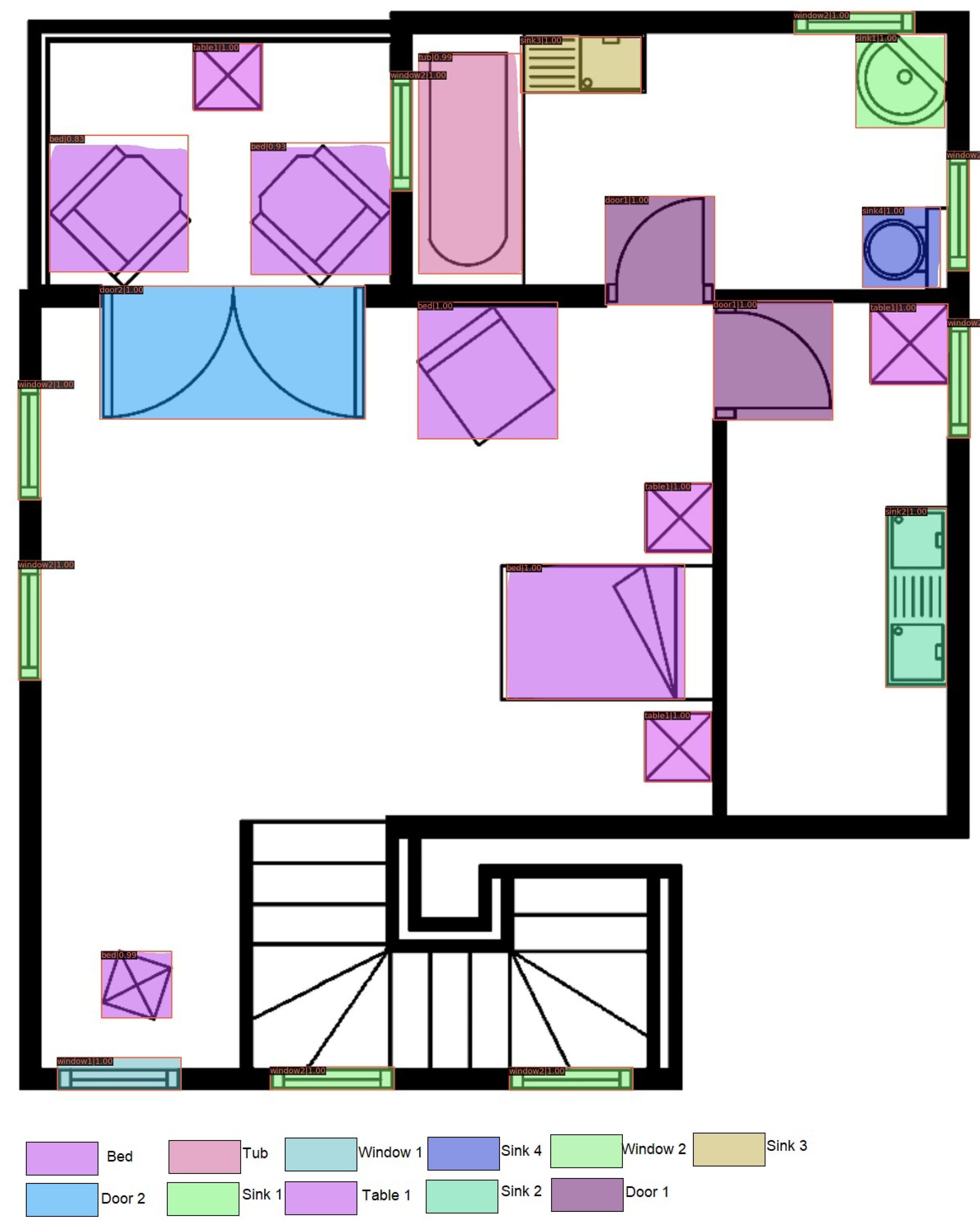
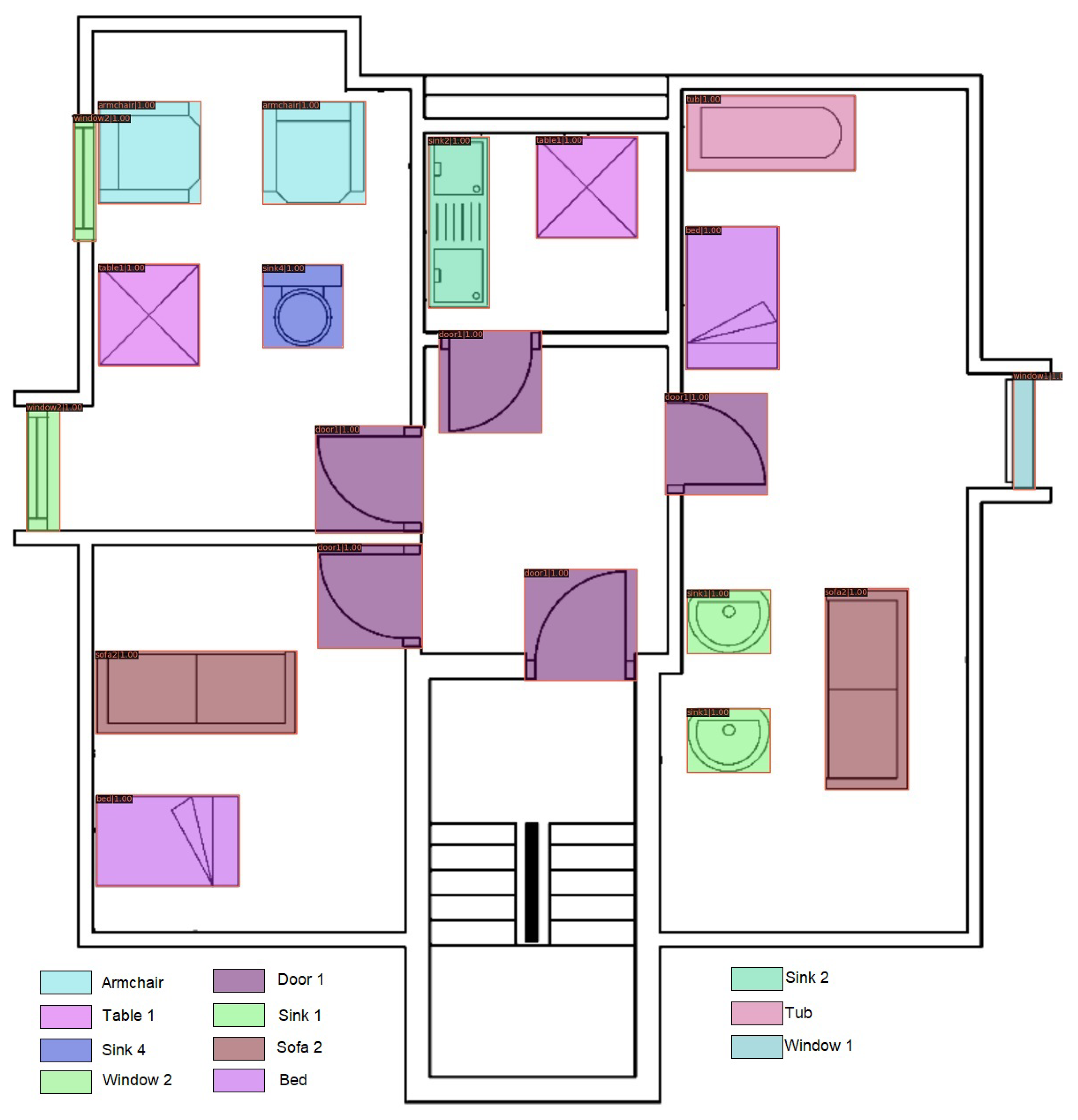
Figure 9 is the output of the experiment Our_SFPI_train_SESYD_test. Few classes are misclassified; for the most part, the network confuses between armchair, sofa, and bed classes. We see many instances where sofa or armchair classes are recognized as the bed. This might be because of the data augmentation we put in the SFPI dataset, whereas in SESYD [3] furniture objects are not that much augmented, and in some scenarios sofa and armchair resembles a bed. To improve the results, we perform our next experiment, Our_SFPI_SESYD_train_SESYD_test, where we use close domain fine-tuning. In Close domain fine-tuning, we fine-tune models using datasets that are closer to the domain of our problem rather than using natural images, which we do when we apply fine-tuning.

In our next experiment Our_SFPI_SESYD_train_SESYD_test, we combine both the SFPI dataset and the SESYD [3] dataset. For training, we use 10,500 images, out of which 10,000 images are from the SFPI dataset, and we pick 500 random images from SESYD [3] dataset. Out of the remaining 500 images of the SESYD [3] dataset, 250 are used for validation, and 250 are used for testing. With the close domain fine-tuning, our model improves, and we get better results. We can achieve a 0.997 mAP score and 0.998 mAR score, which is even better than our experiment Our_SESYD_train_test, where we used the SFPI dataset only for training, validation, and testing. This indicates the advantages of using closed domain fine-tuning.

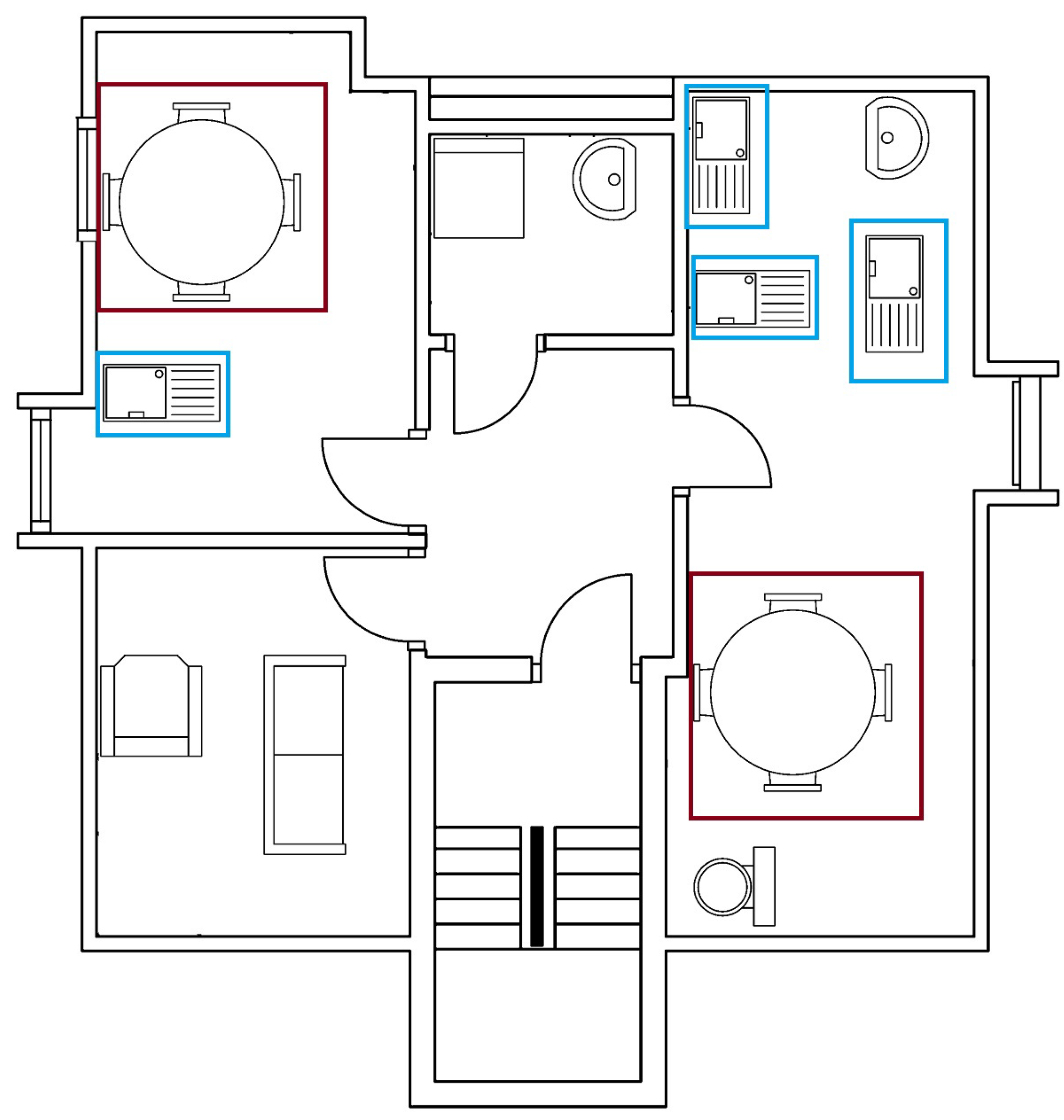
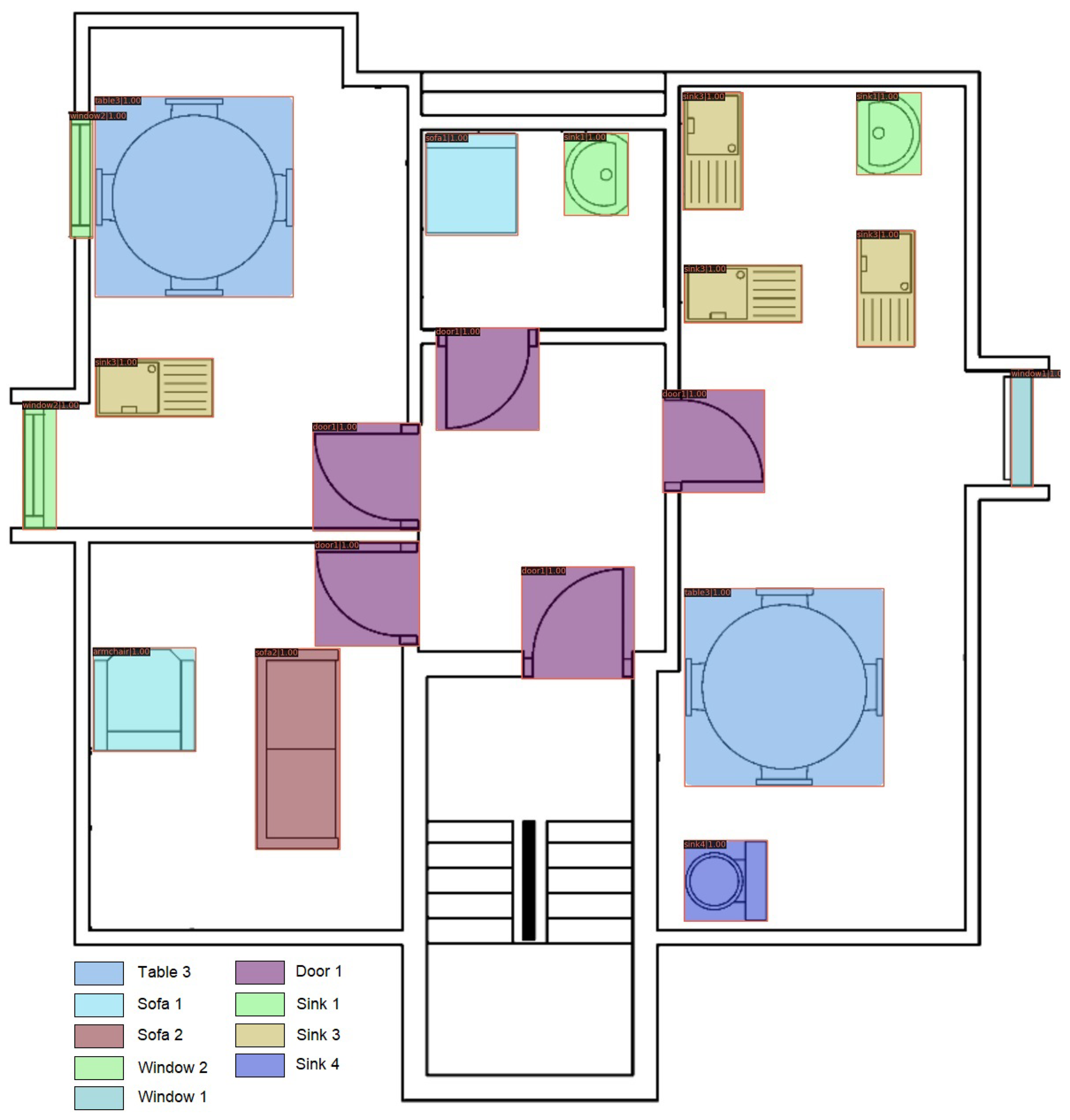
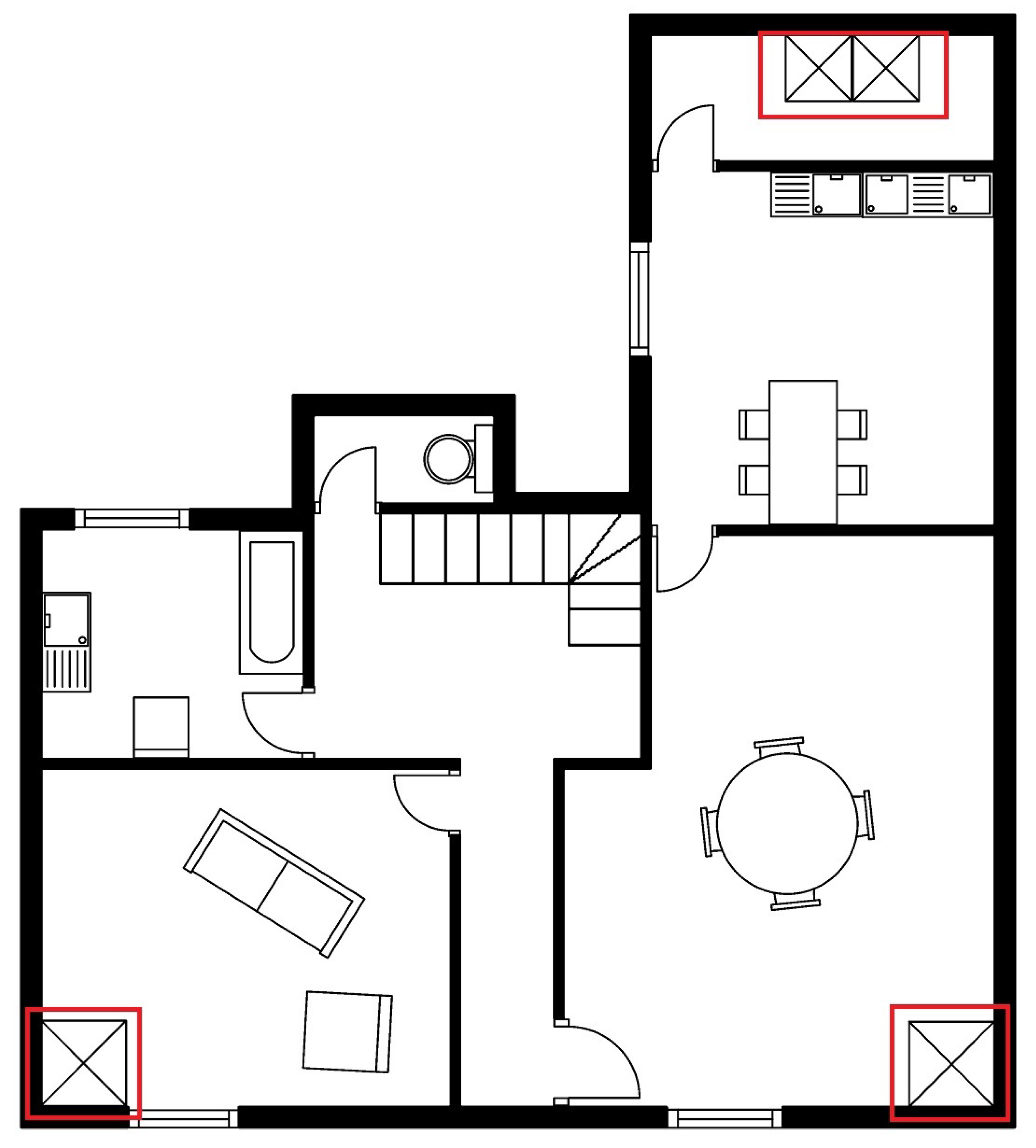
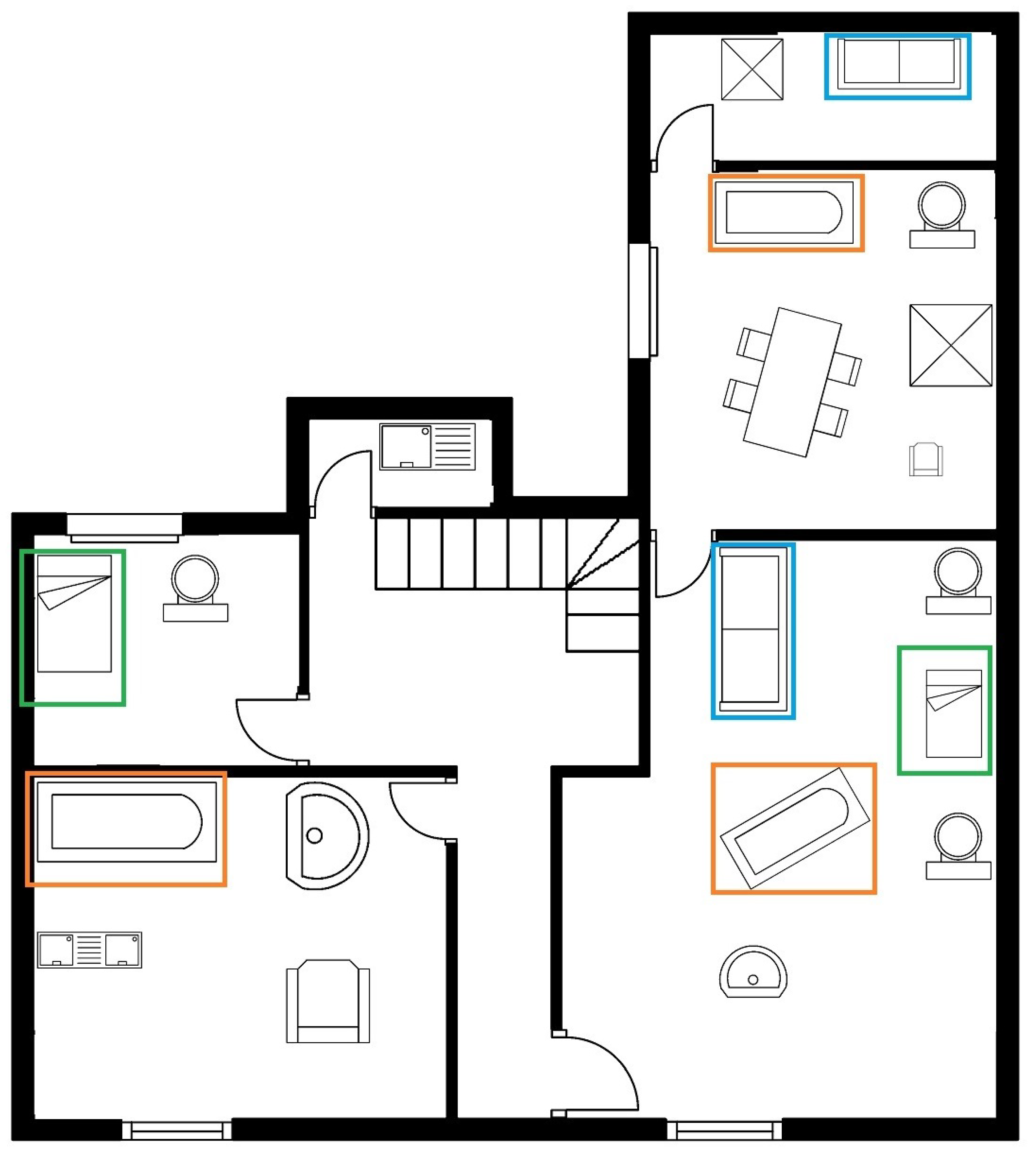
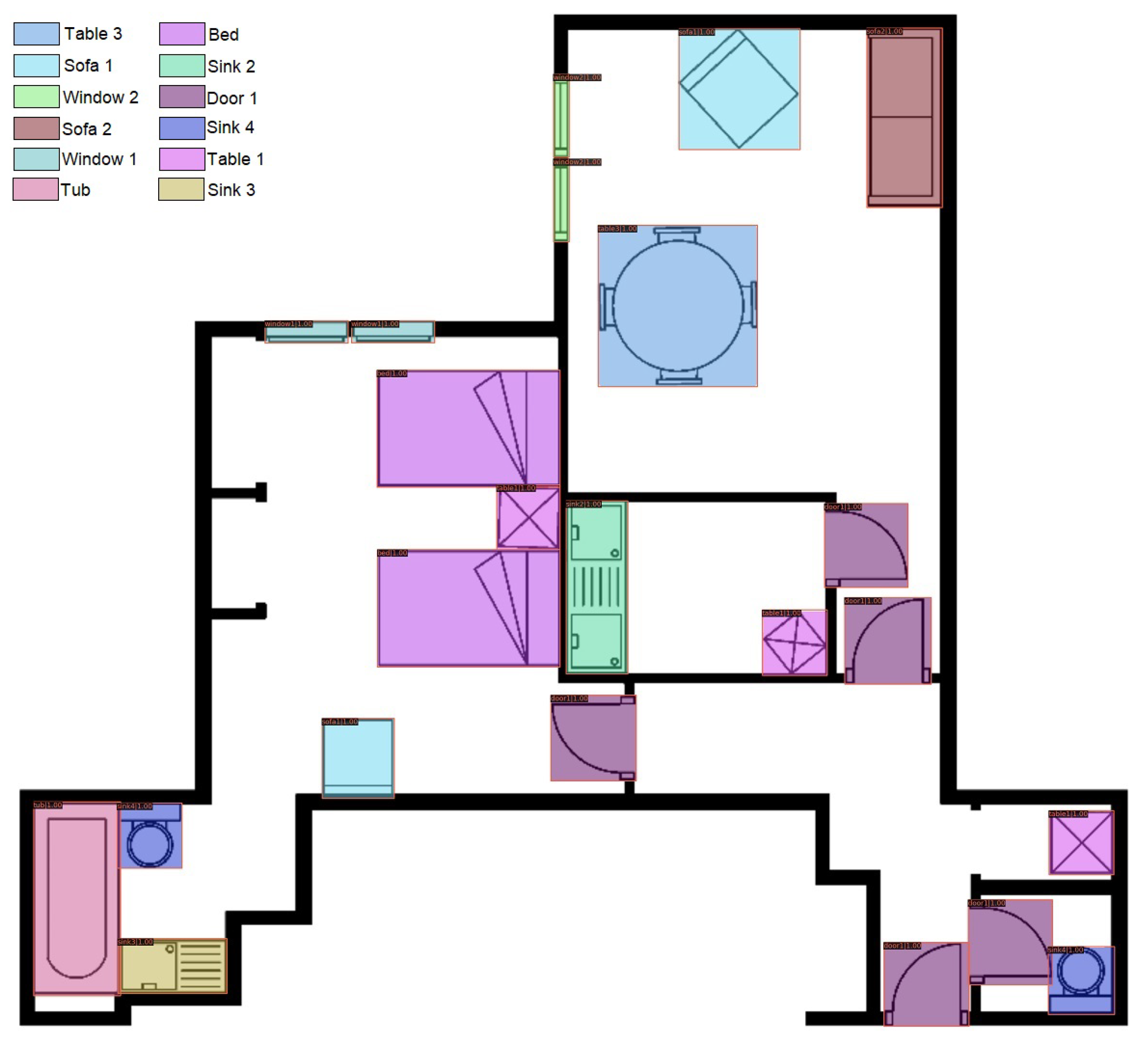
Figure 10 is the final output of our proposed model in the case of experiment Our_SFPI_ SESYD_train_SESYD_test. The image shows that all furniture objects are correctly classified with a good confidence score. In image Figure 10 we can observe good furniture augmentation, as discussed earlier. Our proposed model can generalize well given the context of the two datasets SFPI and SESYD [3] object detection and localization worked perfectly.

In

Table 6. Class-wise average precision (AP) from Our_SFPI_SESYD_train_SESYD_test experiment results. Few classes have reached the score of one, whereas there is some space for improvement in other classes.

Category	AP	Category	AP	Category	AP
Armchair	0.998	Bed	1.000	Door1	1.000
Door2	1.000	Sink1	0.997	Sink2	0.994
Sink3	0.994	Sink4	0.999	Sofa1	0.997
Sofa2	0.996	Table1	0.999	Table2	0.996
Table3	1.000	Tub	1.000	Window1	0.987
Window2	0.994	-	-	-	-

, we described the class-wise average precision score achieved in our experiment Our_SFPI_SESYD_train_SESYD_test. It is visible from the Table 6 that for few classes, we have reached the average precision of one like Door, Bed, and Tub, whereas for the other remaining classes, the score is high, and except Window1 class, all other classes already reached above 0.90 average precision. This class-wise AP result gives us more clarity about model performance. We can identify where our model works well and what classes are causing problems.

For completeness of the paper, we computed the mAP score on various IoU thresholds ranging from 0.5 to 1.0. We performed this for all of our three experiments. Figure 11 illustrates the performance of our approach in terms of mean average precision. We can see that we can achieve mAP score of one for Our_SESYD_train_test, 0.861 in the case of Our_SFPI_train_SESYD_test, and 0.936 for Our_SFPI_SESYD_train_SESYD_test when the IoU is set to 0.5. From this point onwards, as we increase, the IoU mAP is decreasing for the latter mentioned two experiments. For experiment Our_SFPI_train_SESYD_test and experiment Our_SFPI_SESYD_train_SESYD_after the IoU threshold of 0.8, mAP is equal. The mAP score eventually reaches zero when we set the IoU to 1 for all experiments.

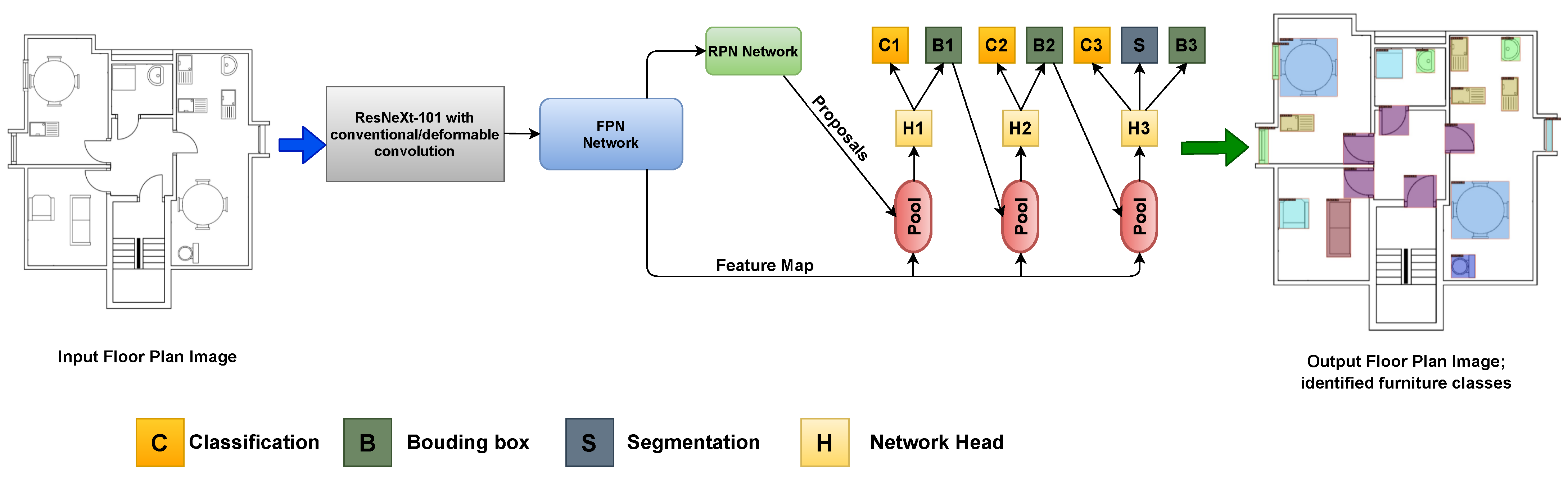
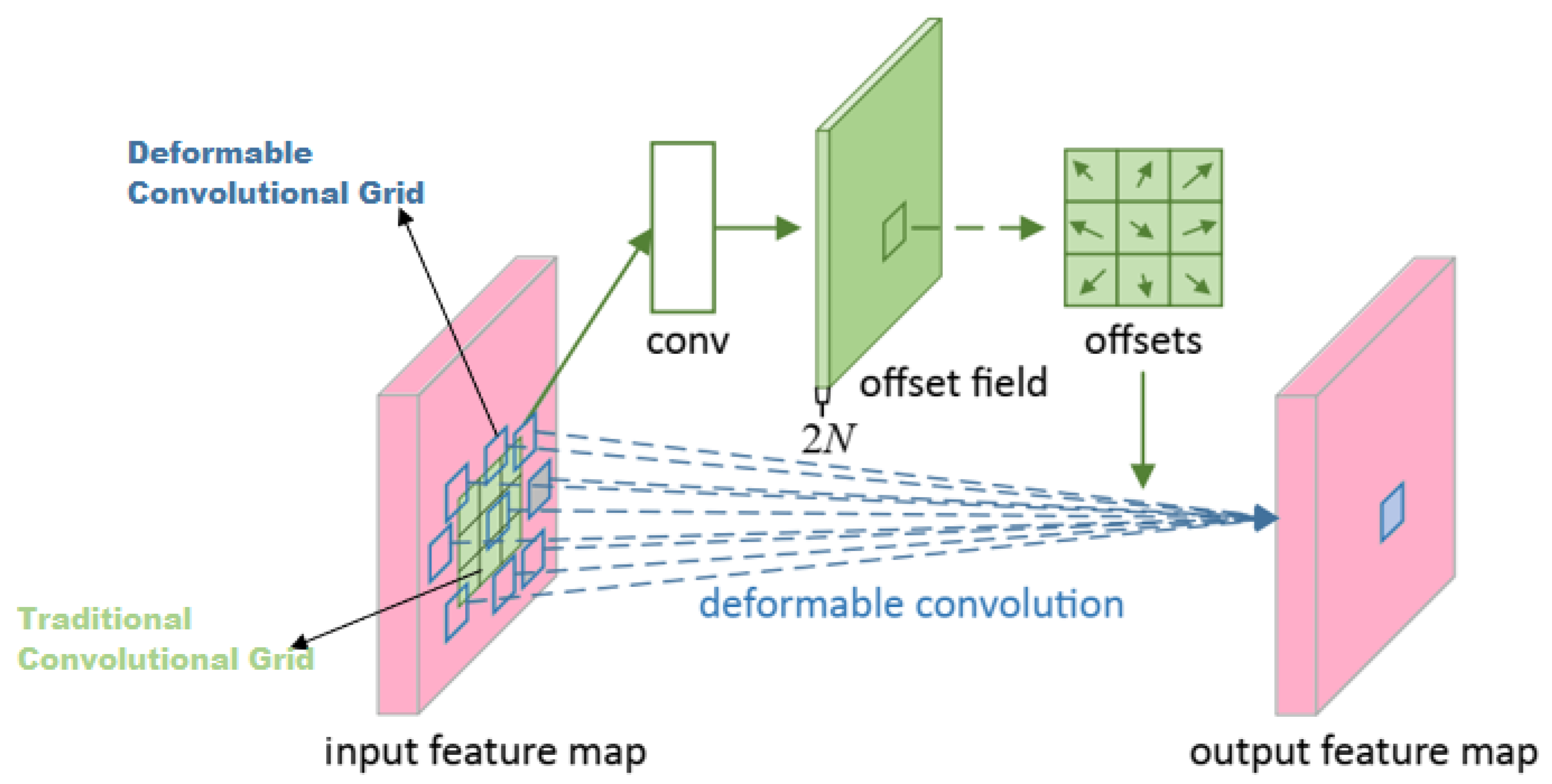
Until this point, we were only deploying conventional convolutional networks, but we want to apply our model with deformable convolution network (DCN) [16] as well. DCN [16] could be useful for our datasets as they can easily adapt the shape of unknown complex transformations in the input. DCN’s [16] are helpful when we have huge data augmentation in the dataset, to identify different transformations of the same objects. We performed all three experiments with backbone ResNeXt-101 [17] along with deformable convolutions [16]. All other specifications of the experiments such as dataset split and Cascade Mask R-CNN [15] remain the same as they are for backbone ResNeXt-101 [17] with traditional convolution (CNN).

In

Table 7. Performance analysis of the proposed model on different experiments performed with conventional convolution (CNN) and deformable convolution (DCN) [16] backbone.

		Mean Average Precision (mAP)		Mean Average Recall (mAR)
Method	Type	Val	Test	Val	Test
Our_SESYD_train_test	CNN	0.981	0.982	0.986	0.987
Our_SFPI_train_test	CNN	0.995	0.995	0.997	0.997
	DCN [16]	0.998	0.998	0.999	0.999
Our_SFPI_train_SESYD_test	CNN	0.751	0.750	0.775	0.775
	DCN [16]	0.768	0.763	0.788	0.783
Our_SFPI_SESYD_train_SESYD_test	CNN	0.997	0.997	0.998	0.998
	DCN [16]	0.998	0.998	0.999	0.999

, we present the quantitative analysis of all experiments we have performed with our end-to-end model. We can identify that using deformable convolution [16] enhances the results of our model. In our experiment Our_SESYD_train_test with conventional convolution (CNN), we can achieve a mAP of 0.995 and a mAR of 0.997, whereas when we changed the backbone to use deformable convolution [16], the overall score improved to 0.998 for mAP and 0.999 for mAR, which is close to the perfect score. For our experiment, our_SFPI_train_SESYD_test, where we are using the SFPI dataset for training and the SESYD [3] dataset for testing and validation, with CNN backbone, we get a score of 0.750 for mAP and 0.775 for mAR, whereas when we used a deformable convolution [16], the score improved, and we obtained 0.763 for mAP and 0.783 for mAR. This indicates that deformable convolution can be helpful to get more generalized object detection. In our experiment Our_SFPI_SESYD_train_SESYD_test, we performed closed domain fine-tuning on our model and achieved our best result until now, which was a 0.997 score for mAP and 0.998 score for mAR. This further improves when we use a deformable convolution [16] for closed domain fine-tuning; we achieved a score of 0.998 for mAP and 0.999 for mAR. This is the best result among all experiments we performed on the SFPI dataset, as well as other experiments we came across during the literature survey for object detection in floor plan images.

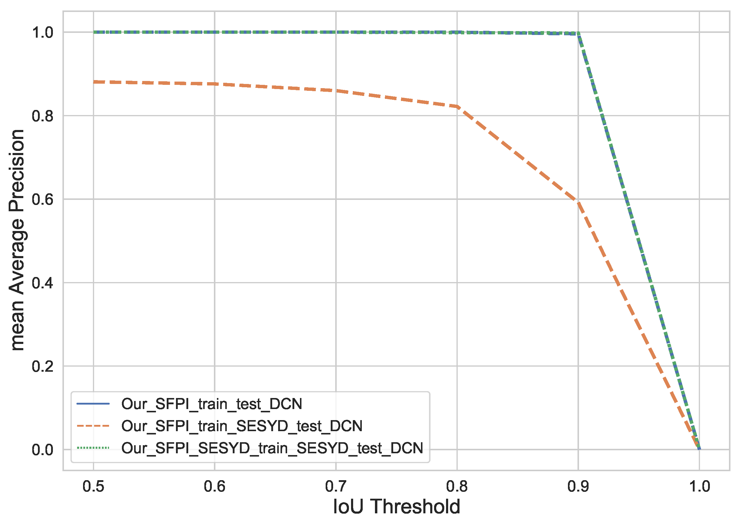
We perform all our experiments with backbone ResNeXt-101 [17] combining deformable convolutions (DCN) [16] on different IoU thresholds. Figure 12 depicts the performance of our model during each experiment on different IoU thresholds. Our_SFPI_train_test and Our_SFPI_SESYD_train_SESYD_test result in the same mAP score, whereas for Our_SFPI_train_SESYD_test, we start with a mAP score of 0.881 for 0.5 IoU threshold. Our_SFPI_train_test and Our_SFPI_SESYD_train_SESYD_test gives a constant mAP score until the IoU threshold 0.9, whereas we see a constant decrease in the mAP score of Our_SFPI_train_SESYD_test. Eventually, all three experiments will end up on a mAP score of zero when we set the IoU to 1. The final output of experiment Our_SFPI_SESYD_train_ SESYD_test_DCN is available in the Figure 13.

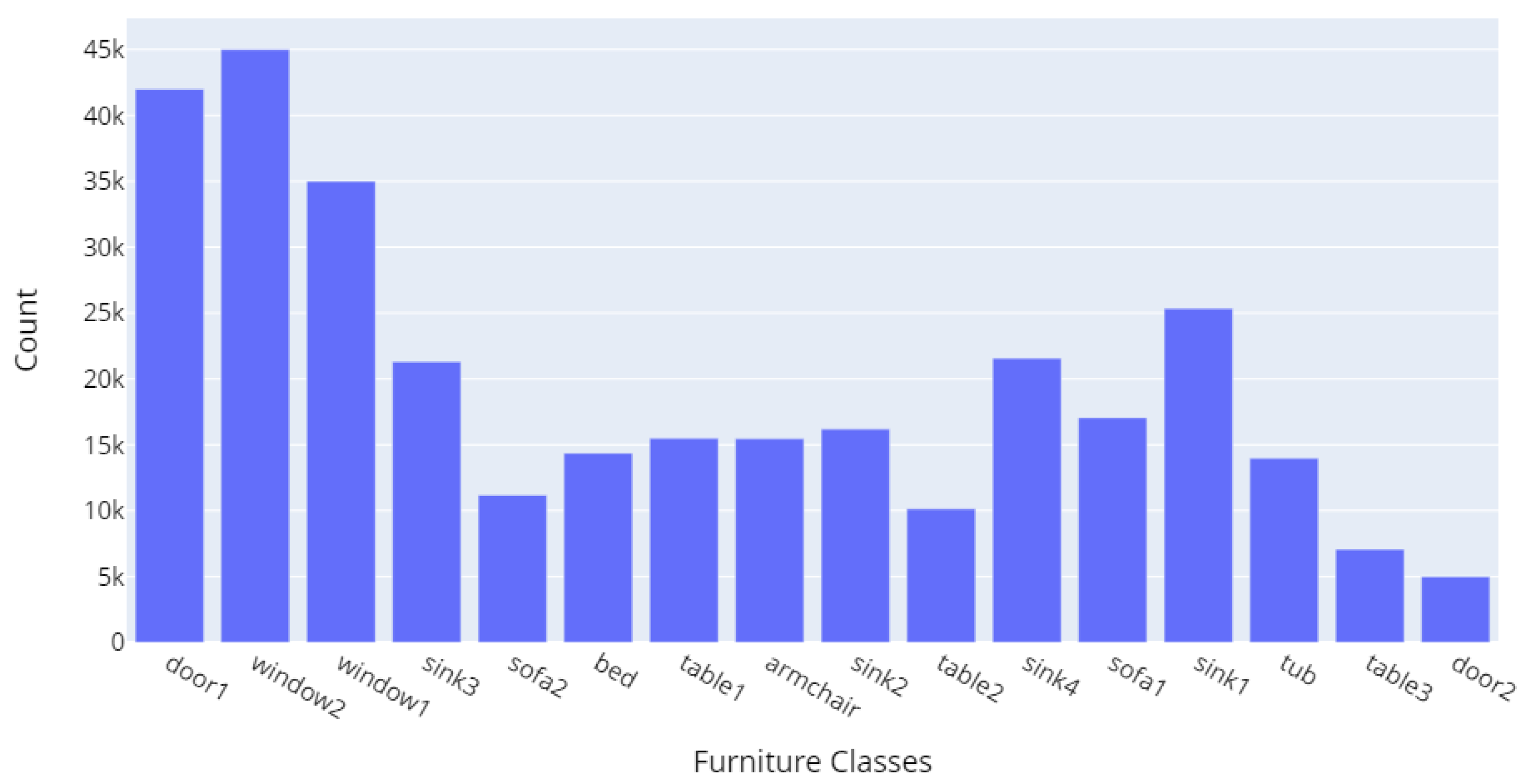
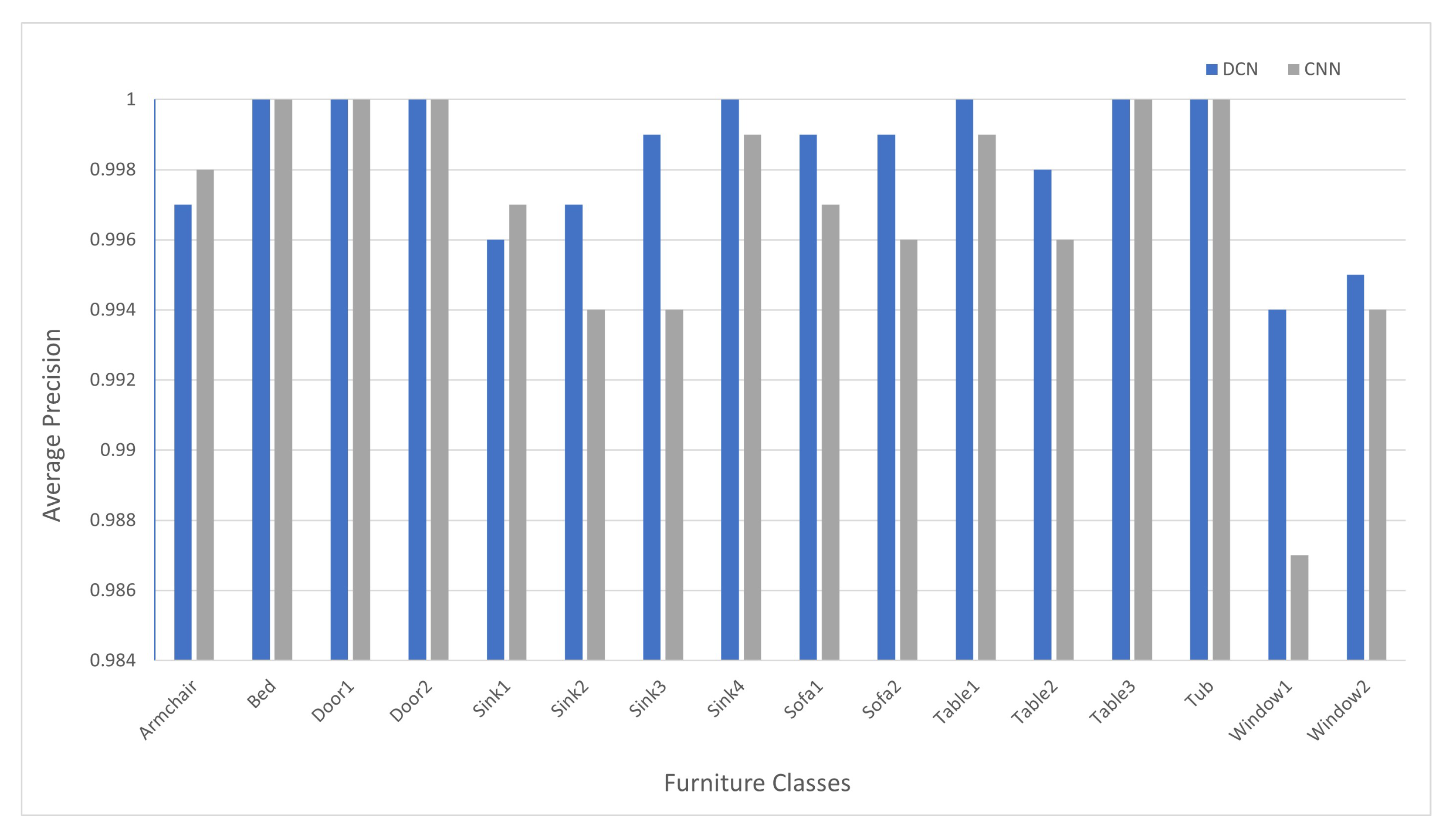
We can take a better look at individual furniture classes with respective accuracy in

Table 8. Class-wise average precision (AP) from the results of our experiment Our_SFPI_SESYD_train_SESYD_test_ DCN.

Category	AP	Category	AP	Category	AP
Armchair	0.997	Bed	1.000	Door1	1.000
Door2	1.000	Sink1	0.996	Sink2	0.997
Sink3	0.999	Sink4	1.000	Sofa1	0.999
Sofa2	0.999	Table1	1.000	Table2	0.998
Table3	1.000	Tub	1.000	Window1	0.994
Window2	0.995	-	-	-	-

. Comparing this result Table 8 with the class-wise result we have obtained in Table 6 improvements are clearly visible. Comparison of these two class-wise results is available in Figure 14. The figure illustrates that scores for Sink2 and Sink3 furniture classes have been improved. When we verify the images of these two classes, we can recognize that these classes have many similarities, and using DCN helps our model differentiate and recognize each class more precisely. We can also see the major improvement in Window1 and Window2 classes; these classes are also difficult to distinguish, and that is where we take advantage of deformable convolution [16] to improve the overall score. In conclusion, we can see that most of the furniture classes either have a score of one or close to one.

6. Conclusions and Future Work

We introduce an end-to-end trainable network for detecting furniture objects in floor plan images. Our proposed method incorporates the high-level architectural principle of traditional object detection approaches. Specifically, we exploit and compare traditional convolution and deformable convolution approaches to detect furniture objects in the floor plan images using Cascade Mask R-CNN [15]. Our different experiments and modifications will help to achieve better generalization and detection performance. We achieve state-of-the-art performance on COCO primary challenge matrices (AP at IoU = 0.50:0.05:0.95) with the mAP score of 0.998 on our SFPI dataset. With our proposed method, we achieved a mAP score of 0.982 on the publicly available SESYD [3] dataset. Our literature survey identified no significant public dataset available for floor plan images that can be used to train deep learning detectors. We try filling this gap by creating a custom dataset SFPI containing 10,000 floor plan images with 316,160 object instances available in these images. There are 16 different furniture classes and ten different floor plans. This dataset can be further extended using our scripts and can quickly adapt to new furniture classes. Moreover, the presented work empirically establishes that it is possible to achieve state-of-the-art object detection in floor plan images.

For future work, we expect our SFPI dataset to be embedded with more floor plan layouts and different furniture objects to make a more generalized floor plan dataset. A deeper backbone would be able to improve the performance without using deformable convolution. Moreover, these experiments can be used in different floor plan applications such as interactive image-fitting and floor plan text generation, helping visually impaired people with floor plans. Earlier, all these applications used Faster R-CNN [12], but now with our experiments, it is evident that Cascade Mask R-CNN [15] performs better in these applications.

References

1. Kang, K.; Ouyang, W.; Li, H.; Wang, X. Object detection from video tubelets with convolutional neural networks. In Proceedings of the IEEE Conference on Computer Vision and Pattern Recognition, Las Vegas, NV, USA, 27–30 June 2016; pp. 817–825. [Google Scholar]
2. Ahmed, M.; Hashmi, K.A.; Pagani, A.; Liwicki, M.; Stricker, D.; Afzal, M.Z. Survey and Performance Analysis of Deep Learning Based Object Detection in Challenging Environments. Sensors 2021, 21, 5116. [Google Scholar] [CrossRef]
3. Delalandre, M.; Valveny, E.; Pridmore, T.; Karatzas, D. Generation of synthetic documents for performance evaluation of symbol recognition & spotting systems. Int. J. Doc. Anal. Recognit. (IJDAR) 2010, 13, 187–207. [Google Scholar]
4. Gimenez, L.; Robert, S.; Suard, F.; Zreik, K. Automatic reconstruction of 3D building models from scanned 2D floor plans. Autom. Constr. 2016, 63, 48–56. [Google Scholar] [CrossRef]
5. Gimenez, L.; Hippolyte, J.L.; Robert, S.; Suard, F.; Zreik, K. reconstruction of 3D building information models from 2D scanned plans. J. Build. Eng. 2015, 2, 24–35. [Google Scholar] [CrossRef]
6. Ahmed, S.; Liwicki, M.; Weber, M.; Dengel, A. Automatic room detection and room labeling from architectural floor plans. In Proceedings of the 2012 10th IAPR International Workshop on Document Analysis Systems, Gold Coast, QLD, Australia, 27–29 March 2012; pp. 339–343. [Google Scholar]
7. De las Heras, L.P.; Terrades, O.; Robles, S.; Síanchez, G. CVC-FP and SGT: A new database for structural floor plan analysis and its groundtruthing tool. Int. J. Doc. Anal. Recognit. 2015, 18, 15–30. [Google Scholar] [CrossRef]
8. GitHub, I. Open Source Survey. 2017. Available online: https://github.com/gesstalt/ROBIN (accessed on 21 July 2021).
9. Ziran, Z.; Marinai, S. Object detection in floor plan images. In Lecture Notes in Computer Science, Proceedings of the IAPR Workshop on Artificial Neural Networks in Pattern Recognition, Siena, Italy, 19–21 September 2018; Springer: Cham, Switzerland, 2018; pp. 383–394. [Google Scholar]
10. Dodge, S.; Xu, J.; Stenger, B. Parsing floor plan images. In Proceedings of the 2017 Fifteenth IAPR International Conference on Machine Vision Applications (MVA), Nagoya, Japan, 8–12 May 2017; pp. 358–361. [Google Scholar]
11. Lv, X.; Zhao, S.; Yu, X.; Zhao, B. Residential Floor Plan Recognition and Reconstruction. In Proceedings of the IEEE/CVF Conference on Computer Vision and Pattern Recognition (CVPR), Nashville, TN, USA, 19–25 June 2021; pp. 16717–16726. [Google Scholar]
12. Ren, S.; He, K.; Girshick, R.; Sun, J. Faster R-CNN: Towards real-time object detection with region proposal networks. IEEE Trans. Pattern Anal. Mach. Intell. 2016, 39, 1137–1149. [Google Scholar] [CrossRef] [PubMed] [Green Version]
13. Redmon, J.; Farhadi, A. YOLO9000: Better, faster, stronger. In Proceedings of the IEEE Conference on Computer Vision and Pattern Recognition, Honolulu, HI, USA, 21–26 July 2017; pp. 7263–7271. [Google Scholar]
14. Hurtik, P.; Števuliáková, P. Pattern matching: Overview, benchmark and comparison with F-transform general matching algorithm. Soft Comput. 2017, 21, 3525–3536. [Google Scholar] [CrossRef]
15. Cai, Z.; Vasconcelos, N. Cascade R-CNN: High Quality Object Detection and Instance Segmentation. IEEE Trans. Pattern Anal. Mach. Intell. 2019, 43, 1483–1498. [Google Scholar] [CrossRef] [PubMed] [Green Version]
16. Dai, J.; Qi, H.; Xiong, Y.; Li, Y.; Zhang, G.; Hu, H.; Wei, Y. Deformable Convolutional Networks. In Proceedings of the IEEE International Conference on Computer Vision, Venice, Italy, 22–29 October 2017. [Google Scholar]
17. Xie, S.; Girshick, R.; Dollar, P.; Tu, Z.; He, K. Aggregated Residual Transformations for Deep Neural Networks. In Proceedings of the IEEE Conference on Computer Vision and Pattern Recognition (CVPR), Honolulu, HI, USA, 21–26 July 2017. [Google Scholar]
18. Krizhevsky, A.; Sutskever, I.; Hinton, G.E. Imagenet classification with deep convolutional neural networks. Adv. Neural Inf. Process. Syst. 2012, 25, 1097–1105. [Google Scholar] [CrossRef]
19. He, K.; Zhang, X.; Ren, S.; Sun, J. Deep residual learning for image recognition. In Proceedings of the IEEE Conference on Computer Vision and Pattern Recognition, Las Vegas, NV, USA, 26 June–1 July 2016; pp. 770–778. [Google Scholar]
20. Zhang, C.L.; Xu, Y.P.; Xu, Z.J.; He, J.; Wang, J.; Adu, J.H. A fuzzy neural network based dynamic data allocation model on heterogeneous multi-GPUs for large-scale computations. Int. J. Autom. Comput. 2018, 15, 181–193. [Google Scholar] [CrossRef] [Green Version]
21. Téllez-Velázquez, A.; Cruz-Barbosa, R. A CUDA-streams inference machine for non-singleton fuzzy systems. Concurr. Comput. Pract. Exp. 2018, 30, e4382. [Google Scholar] [CrossRef]
22. De las Heras, L.P.; Ahmed, S.; Liwicki, M.; Valveny, E.; Sánchez, G. Statistical segmentation and structural recognition for floor plan interpretation. Int. J. Doc. Anal. Recognit. (IJDAR) 2014, 17, 221–237. [Google Scholar] [CrossRef]
23. Hashmi, K.A.; Pagani, A.; Liwicki, M.; Stricker, D.; Afzal, M.Z. CasTabDetectoRS: Cascade Network for Table Detection in Document Images with Recursive Feature Pyramid and Switchable Atrous Convolution. J. Imaging 2021, 7, 214. [Google Scholar] [CrossRef]
24. Hashmi, K.A.; Pagani, A.; Liwicki, M.; Stricker, D.; Afzal, M.Z. Cascade Network with Deformable Composite Backbone for Formula Detection in Scanned Document Images. Appl. Sci. 2021, 11, 7610. [Google Scholar] [CrossRef]
25. Liu, Y.; Wang, Y.; Wang, S.; Liang, T.; Zhao, Q.; Tang, Z.; Ling, H. Cbnet: A novel composite backbone network architecture for object detection. In Proceedings of the AAAI Conference on Artificial Intelligence, New York, NY, USA, 7–12 February 2020; Volume 34, pp. 11653–11660. [Google Scholar]
26. Lin, T.Y.; Maire, M.; Belongie, S.; Hays, J.; Perona, P.; Ramanan, D.; Dollár, P.; Zitnick, C.L. Microsoft coco: Common objects in context. In Lecture Notes in Computer Science, Proceedings of the European Conference on Computer Vision, Zurich, Switzerland, 6–12 September 2014; Springer: Cham, Switzerland, 2014; pp. 740–755. [Google Scholar]
27. Wang, C.W.; Cheng, C.A.; Cheng, C.J.; Hu, H.N.; Chu, H.K.; Sun, M. Augpod: Augmentation-oriented probabilistic object detection. In Proceedings of the CVPR Workshop on the Robotic Vision Probabilistic Object Detection Challenge, Long Beach, CA, USA, 17 June 2019. [Google Scholar]
28. He, W.; Li, C.; Nie, X.; Wei, X.; Li, Y.; Li, Y.; Luo, S. Recognition and detection of aero-engine blade damage based on Improved Cascade Mask R-CNN. Appl. Opt. 2021, 60, 5124–5133. [Google Scholar] [CrossRef] [PubMed]
29. Kumar, D.; Zhang, X. Improving More Instance Segmentation and Better Object Detection in Remote Sensing Imagery Based on Cascade Mask R-CNN. In Proceedings of the 2021 IEEE International Geoscience and Remote Sensing Symposium IGARSS, Brussels, Belgium, 11–16 July 2021; pp. 4672–4675. [Google Scholar]
30. Lee, J.; Lee, S.; Back, S.; Shin, S.; Lee, K. Object Detection for Understanding Assembly Instruction Using Context-aware Data Augmentation and Cascade Mask R-CNN. arXiv 2021, arXiv:2101.02509. [Google Scholar]
31. Eklund, A. Cascade Mask R-CNN and Keypoint Detection used in Floorplan Parsing. Master’s Thesis, Uppsala University, Uppsala, Sweden, 24 June 2020. [Google Scholar]
32. Goyal, S.; Chattopadhyay, C.; Bhatnagar, G. Plan2Text: A framework for describing building floor plan images from first person perspective. In Proceedings of the 2018 IEEE 14th International Colloquium on Signal Processing Its Applications (CSPA), Penang, Malaysia, 9–10 March 2018; pp. 35–40. [Google Scholar] [CrossRef]
33. Zeng, Z.; Li, X.; Yu, Y.K.; Fu, C.W. Deep Floor Plan Recognition Using a Multi-Task Network With Room-Boundary-Guided Attention. In Proceedings of the IEEE/CVF International Conference on Computer Vision (ICCV), Seoul, Korea, 27 October–2 November 2019. [Google Scholar]
34. Simonyan, K.; Zisserman, A. Very Deep Convolutional Networks for Large-Scale Image Recognition. arXiv 2015, arXiv:1409.1556. [Google Scholar]
35. Bochkovskiy, A.; Wang, C.Y.; Liao, H.Y.M. Yolov4: Optimal speed and accuracy of object detection. arXiv 2020, arXiv:2004.10934. [Google Scholar]
36. Chen, K.; Wang, J.; Pang, J.; Cao, Y.; Xiong, Y.; Li, X.; Sun, S.; Feng, W.; Liu, Z.; Xu, J.; et al. MMDetection: Open mmlab detection toolbox and benchmark. arXiv 2019, arXiv:1906.07155. [Google Scholar]
37. Lin, T.Y.; Dollár, P.; Girshick, R.; He, K.; Hariharan, B.; Belongie, S. Feature pyramid networks for object detection. In Proceedings of the IEEE Conference on Computer Vision and Pattern Recognition, Honolulu, HI, USA, 21–26 July 2017; pp. 2117–2125. [Google Scholar]
38. Zhuge, Y.; Ciesielski, K.C.; Udupa, J.K.; Miller, R.W. GPU-based relative fuzzy connectedness image segmentation. Med. Phys. 2013, 40, 011903. [Google Scholar] [CrossRef] [Green Version]
39. Everingham, M.; Van Gool, L.; Williams, C.K.; Winn, J.; Zisserman, A. The pascal visual object classes (voc) challenge. Int. J. Comput. Vis. 2010, 88, 303–338. [Google Scholar] [CrossRef] [Green Version]
40. Powers, D.M.W. Evaluation: From precision, recall and F-measure to ROC, informedness, markedness and correlation. arXiv 2020, arXiv:2010.16061. [Google Scholar]
Figure 1. Sample floor plan image with the specification of different room sizes and furniture objects. Each variety of floor plan layout has different floor plan elements, shapes, and sizes.
Applsci 11 11174 g001
Figure 2. Sample floor plan image from SESYD [3] dataset containing various furniture object classes in different rooms. For example, blue boxes represent sink class, whereas red boxes highlight table class.
Applsci 11 11174 g002
Figure 3. Sample floor plan image with ground truth. Various furniture class objects available in the image are highlighted.
Applsci 11 11174 g003
Figure 4. The presented framework is based on Cascade Mask R-CNN [15] equipped with ResNeXt-101 [17] backbone with conventional and deformable convolution applied on floor plan images. Modules B, C, and S represent bounding box, classification, and segmentation, respectively.
Applsci 11 11174 g004
Figure 5. Internal working of deformable convolution [16]. The light green grid on the input feature map shows the conventional 3 × 3 convolutional operation, whereas the blue boxes on the input feature map show the effective receptive field of a 3 × 3 deformable convolution.
Applsci 11 11174 g005
Figure 6. Sample image from SESYD [3] dataset. Minimal variation in the furniture objects. It is visible from the red highlighted objects of Table class that these objects do not vary in orientation or scale.
Applsci 11 11174 g006
Figure 7. Sample image from the proposed SFPI dataset. Furniture object’s augmentation is evident, i.e., highlighted Tub and Sofa classes have a couple of objects with different orientations and scales.
Applsci 11 11174 g007
Figure 8. The distribution of different furniture class objects in the SFPI dataset.
Applsci 11 11174 g008
Figure 9. Qualitative results of our proposed model from experiment Our_SFPI_train_SESYD_test. Many miss-classified classes are visible in the image, such as Bed and Sofa.
Applsci 11 11174 g009
Figure 10. Sample output from experiment Our_SFPI_SESYD_train_SESYD_test. It is evident that all furniture objects are identified and localized correctly.
Applsci 11 11174 g010
Figure 11. Mean Average Precision achieved over varying IoU thresholds for different experiments on the proposed method with conventional convolution (CNN).
Applsci 11 11174 g011
Figure 12. Mean Average Precision achieved over varying IoU thresholds for different experiments on the proposed method with DCN [16].
Applsci 11 11174 g012
Figure 13. The qualitative result of our experiment Our_SFPI_SESYD_train_SESYD_test with deformable convolutions [16] on SFPI dataset.
Applsci 11 11174 g013
Figure 14. Class-wise average precision comparison Conventional Convolutional Network (CNN) and Deformable convolutional Network (DCN) [16]. The results have been taken from experiments Our_SFPI_SESYD_train_SESYD_test_CNN and Our_SFPI_SESYD_train_SESYD_test_ DCN.
Applsci 11 11174 g014