Microstructure-Based Lifetime Assessment of Austenitic Steel AISI 347 in View of Fatigue, Environmental Conditions and NDT

Abstract

The assessment of metallic materials used in power plants’ piping represents a big challenge due to the thermal transients and the environmental conditions to which they are exposed. At present, a lack of information related to degradation mechanisms in structures and materials is covered by safety factors in its design, and in some cases, the replacement of components is prescribed after a determined period of time without knowledge of the true degree of degradation. In the collaborative project “Microstructure-based assessment of maximum service life of nuclear materials and components exposed to corrosion and fatigue (MibaLeb)”, a methodology for the assessment of materials’ degradation is being developed, which combines the use of NDT techniques for materials characterization, an optimized fatigue lifetime analysis using short time evaluation procedures (STEPs) and numerical simulations. In this investigation, the AISI 347 (X6CrNiNb18-10) is being analyzed at different conditions in order to validate the methodology. Besides microstructural analysis, tensile and fatigue tests, all to characterize the material, a pressurized hot water pipe exposed to a series of flow conditions will be evaluated in terms of full-scale testing as well as prognostic evaluation, where the latter will be based on the materials’ data generated, which should prognose changes in the material’s condition, specifically in a pre-cracked stage. This paper provides an overview of the program, while the more material’s related aspects are presented in the subsequent paper.

1. Introduction

Damage is an expression generally used when a material is exposed to loading. However, its meaning is extremely wide, and the mechanisms damage is based upon are versatile. Description, measurement, and quantification of damage in a material is therefore highly complex and requires a systematic to be well thought through, specifically from the material’s microstructure point of view.

Within the joint national research project “Microstructure-based assessment of maximum service duration of nuclear materials and components exposed to corrosion and fatigue (MibaLeb)” funded by the German Federal Ministry of Economic Affairs and Energy (BMWi), the austenitic stainless steel AISI 347 (X6CrNiNb18-10), widely used for piping in German nuclear power plants, has been analyzed and characterized from a microstructural point of view. A series of constant amplitude fatigue tests (CAT), as well as load and strain increase fatigue tests (LIT and SIT), were performed under various loading, temperature and environmental conditions, where not only load and deformation had been recorded but also parameters associated with non-destructive testing (NDT), taken as a material response for the description of the material’s damaging behavior. These fatigue tests were performed following short time evaluation procedures (STEP), that allow a complete S-N curve of a material to be determined with three tests only.

A material’s response recorded through NDT-based parameters needs the recorded signals to be analyzed in the first place before extracting features from those signals, that may be related to the different damage mechanisms that occur during the test. It is important to obtain a good understanding of how damage develops for every condition to be assessed for the material being considered. In MibaLeb, differentiation has been done concerning temperature (room temperature (RT) and elevated temperature at 240 and 300 °C), the fatigue regime (low (LCF) and high cycle fatigue (HCF)), and the type of control (load versus strain control). Other factors like the strain/stress amplitude or the strain/stress rate may affect the material’s response as well.

Based on the Ni and Cr content of the AISI 347 (X6CrNiNb18-10) and using the Strauss-Maurer microstructure diagram, a metastable γ-austenite microstructure after standard heat treatment is to be expected.

When the material is subjected to strain controlled cyclic loading at RT, the paramagnetic γ-austenite can transform into ferromagnetic α’-martensite [1]. It has been shown that in the LCF regime, this phase transformation reduces the fatigue life of the specimen, mainly for two reasons: the formation involves the change from a face-centered cubic (fcc) structure to a body-centered tetragonal (bct) structure, which is a distorted form of a body-centered-cubic (bcc) structure [2], increasing its volume and producing a highly stressed structure, harder and more brittle than the austenite [3]. Furthermore, the martensite is expected to act as a preferential crack initiation site. In contrast, in the HCF regime, the fatigue life is increased, given the nucleation of very fine martensite particles in the area of local plasticity, hindering the dislocation movements [4]. With respect to cyclic softening and/or hardening behavior, it has been shown in [1] that in the LCF regime, for tests conducted at strains in the range of ${\epsilon }_{a,t}=$ 0.6 to 1.6% only cyclic hardening takes place. On the other hand, it has been shown in [5] after analyzing stress amplitude, mean stress and plastic strain amplitude curves of strain-controlled fatigue tests conducted at different strain amplitudes in the HCF regime (${\epsilon }_{a,t}=$ 0.165 to 0.220%), that at the beginning of the test, cyclic softening occurs, followed by cyclic hardening. For both LCF and HCF regimes, there is an incubation period where no α’-martensite transformation takes place, followed by a continuous increase in the α’-martensite volume fraction. The duration of the incubation period decreases with higher total strain amplitudes, contrary to the measured α’-martensite volume fraction at the end of the tests, which increases. Moreover, two austenitic steels of the same type, of which the chemical composition and mechanical properties comply with the standardized limits, but which have differences in chemical composition and grain size, can present substantial differences in the α’-martensite transformation rate and the α’-martensite volume fraction achieved at the end of the test, when tested under the same conditions, which can be explained through the different materials’ metastability.

At an elevated temperature of T > 200 °C, no α’-martensite formation occurs in the LCF and HCF regimes. Furthermore, the cyclic deformation behavior is characterized by initial cyclic hardening and depending on the applied strain amplitude, a subsequent cyclic softening occurs.

The detection of the degradation mechanisms described above relies on the sensitivity of the selected NDT method to those. The motivation of the research is, that mechanical and thermal stresses due to operational conditions together with corrosive influences lead to aging and degradation of a structural material, where the resulting damage can be associated to microstructural changes. The effects of such changes are currently covered rather generally by safety factors in the design of components. Additional qualified information about the microstructural state obtained through monitoring could therefore improve the assessment of an aging condition and better differentiate within the safety margins traditionally set, allowing a component’s residual life evaluation to be enhanced without compromising the level of safety.

What this paper will also elaborate on is the transfer of materials’ data such as generated on unnotched specimens into fatigue life evaluations of notched specimens. Classical approaches such as the one proposed by Neuber will be discussed. It will be shown how local assessment in notched specimens can be made. Based on a plasticity model obtained through finite element simulations and application of the Chaboche model, a further correlation can be established between deformation measurements outside of a notch and local stresses and strains within the notch. With this model, the deformation measured through an external extensometer is related to the local strain using a polynomial function. The plasticity model-based notch root strain and the Neuber approach represent two complementary approaches, allowing local stresses and strains in notched specimens to be assessed.

2. Materials Characterization as a Basis of Structural Integrity Assessment

To get engineering structures assessed regarding their integrity, a material’s behavior has to be known. This becomes specifically essential when a material ages and when a material’s condition changes gradually. Such a change is also often associated with damage, where damage has to be specified accordingly. A further expression in that regard is degradation, where the word itself already implies that the ‘grade’ of the material has been reduced. While the word ‘damage’ has a clear negative touch, the word ‘degradation’ is more quantifiable. The word ‘degradation’ may therefore be used for a phenomenon, which is generally observed when materials and structures are used over time.

When a structure is exposed to loading in service, if the loading result from mechanical or environmental loads, it is generally accepted knowledge that a structural material degrades. From a point of view of design, this degradation is accepted to occur, as long as a minimum grade, being equivalent to a respective damage, is not undercut. Such a principle can also be considered as a damage tolerant design, although it may not be expressed as such explicitly. A ‘tolerable damage’—or better ‘tolerable degradation’—is therefore a structural condition at which the structure’s performance is not going to face catastrophic failure.

Material’s degradation due to loading is a continuous accumulation process, that is difficult to describe. In its possibly most simplistic form, it is assumed to be a linear process, such as expressed with the Palmgren-Miner rule applied in the case of fatigue damage accumulation. However, it is endlessly proven through experimental evidence, that damage accumulation—or better degradation—is a non-linear process.

Traditionally, damage in a material is only considered from the crack initiation onwards. The primary reasons are that it can mechanically clearly lead to a structure’s catastrophic failure, that it can be principally monitored visually and that its propagation as a function of loading can be practically described based on modern fracture mechanics. This allows prognostics to be made in terms of a residual life assessment in case an initial condition of degradation is known. This principle has been extended to a structure’s complete fatigue life assessment, where the crack propagation phase being comparatively easier to describe has been merged with the much less known crack-free phase, by simply linearizing the complete degradation process, bearing in mind, that the description of the crack-free phase is associated with a much higher amount of uncertainty, being the major reason why conventional fatigue life evaluations are based on a high degree of uncertainty.

A deeper look into a material’s degradation process during the crack free period elucidates, that the mechanisms are truly versatile. When considering a metallic material, this starts from dislocations in a material that cluster and that further lead to persistent slip bands, starting within grains and gradually growing beyond grain boundaries. For the slip bands on a material’s surface intrusions and extrusions may occur, that become the incubators of cracks in the longer term. The same may apply also inside a material, however, the higher constraints inside the material will prevent cracks to be incubated rather at a later than an early stage. In excess, there may be transformations to occur within a metallic material, such as from austenite to martensite, which is globally observed as a material hardening and where the transformed martensite may build another source of stress concentration and cracking within the material’s microstructure. Reflecting on those degradation processes along the crack-free period of a material’s life endurance is, therefore, most likely far from being linear and is so far only described to a very limited extent.

If the degree of degradation of a material needs to be known, the material needs to be tested. In case no additional damage is to be caused to the material, only non-invasive methods, hence those related to non-destructive testing (NDT), come into play. NDT methods are principally based on mechanical and electromagnetic waves that follow the fundamental physical principles of reflection and transmission, possibly added by some mode conversion. Mechanical waves include the range from classical vibrations up to ultrasound while electromagnetic waves range from radar to gamma rays. The fundamental question now arises as to which of the waves react to the different damage mechanisms (dislocation, slip bands, martensitic transformation, cracks, others) accordingly? This question has to be answered for every case of structural integrity assessment as well as material, such that an optimum solution of structural health monitoring can be developed. This underlines the importance of a microstructural analysis and description of a material’s degradation as well as its link to the physical answers provided by the different NDT techniques.

Today this fundamental interaction between materials science with respect to degradation and NDT, or even broader as the physical monitoring options versus structural integrity assessment, can be still seen to be quite at its infancy. The state-of-the-art principle applied, that loads acting on a structure do lead to cracks and hence degradation, which can be visually inspected (being an NDT technique when professionalized) and where the information monitored can be used to characterize the degree of degradation, which can be used to prognose a component’s residual life until critical failure, is principally correct. However, this approach is affected by a large number of uncertainties, which include, among others:

• the precision of the loads having been monitored,
• the appropriateness of numerically describing a structure’s behavior i.e., the local loading and hence the distribution of stresses, strains and possibly other parameters relevant to degradation,
• the understanding of the damage mechanisms to occur regarding the material’s degradation process,
• the precision to get different damage mechanisms numerically described also in the sense of prognostics,
• the understanding of potential interactions NDT techniques may have with the damage mechanisms to be observed,
• the ability to numerically describe the interactions between NDT techniques and
• the damage mechanisms and any further uncertainties that may arise due to human error once a monitoring concept may have been established.

The MibaLeb project described here is an approach to enhance prognostics of aging infrastructure and to reduce the number of uncertainties referenced above.

3. The MibaLeb Project at a Glance

Engineering infrastructure is exposed to aging, which is a process of degradation. There are numerous examples that can be provided in that regard, where the higher the investment for the infrastructure is, the higher the attention regarding aging becomes. An excellent example in that regard is nuclear engineering infrastructure, such as nuclear power plants. Nuclear power plants are exposed to a harsh loading environment. This includes pressure, temperature, irradiation, corrosion, humidity, to just name a few. This loading leads to mechanical loads on the one side resulting in fatigue and/or creep and into material transformation such as hardening, softening, martensitic transformation, embrittlement, corrosive spalling, deposition and possibly more on the other. All of those conditions and possibly much more have been considered in the design rules set for this nuclear engineering infrastructure including its operational life. Design loads applied have been additionally based on safety factors carefully selected and established in the respective guidelines and standards. However, today, where much of the nuclear engineering infrastructure is coming to the end of its operational design life, the question arises: Has this infrastructure truly achieved its real operational life?

To get this question answered in the context of nuclear engineering, requires an evaluation concept to be established, which is by far not available today. However, some inheritance could be taken in that regard from aviation, where the assessment of aging aircraft became virulent after the Aloha Airlines flight 243 accident in 1988.

To get such an infrastructure’s residual life assessment established requires a large amount of information to be gathered and processed, and a further set of instruments to be made available, that would allow the infrastructure’s actual condition to be diagnosed and its residual operational life including maintenance plans to be prognosed. Compared to the original design rules for such an aging infrastructure established decades before, those new maintenance and hence residual life design rules would be based on the application of the latest knowledge and technology and would take better advantage of the infrastructure’s potential without compromising its safety. The information required to be gathered for such new design and maintenance rules may include the original design rules, maintenance and inspection recordings, and any data being recorded during load tests, material testing, microscopical analysis, non-destructive testing and possibly others. The instruments to be made available for the enhanced ‘redesign’ are on the one hand numerical tools allowing a structure’s geometry, its loading performance, stress, strain and thermal distribution, damage incubation and progression—and hence degradation, and finally the way on how inspection could be made in the longer term. The other part of instruments includes sensing devices to be implemented onto or into the infrastructure considered, allowing loads, temperature, pressure and potential degradation to emerge at critical locations over the infrastructure’s residual life to be recorded. This task revisiting an infrastructures design and maintenance is a tremendous one, which cannot be solved within a single project but does rather represent a paradigm change.

Along this huge task, the MibaLeb project has been established, looking into a specific example as a showcase on how to get the larger task of nuclear engineering infrastructure’s residual life tackled in the longer term. The project that started in 2016 and is now in its second phase, is a collaborative initiative between the five partners Gesellschaft für Anlagen- und Reaktorsicherheit (GRS), LZfPQ at Saarland University, MPA of Stuttgart University, WPT of TU Dortmund University and WWHK of University of Applied Sciences Kaiserslautern, funded by the German Ministry of Economic Affairs (BMWi) within its national nuclear safety R&D program. The showcase being considered is a pressurized hot water pipe made of AISI 347 (X6CrNiNb18-10) as being widely used in German nuclear power plants.

In pipes of the primary cooling system of nuclear power plants, the damage mechanisms result primarily from loading due to mechanical and thermal stresses, which can be both static and dynamic. In the operation of nuclear power plants, thermomechanical fatigue damage is of great concern, especially in austenitic materials, which have a low thermal conductivity, that can result in locally different thermal expansions during temperature stratification in the pipelines. If these thermal expansions lead to a local stress buildup across the yield point of the material, local deformation of the component occurs. Thermal stresses on the piping of light water reactors (LWR) range from 250 °C to 330 °C [6]. Moreover, the influence of the LWR environment on the fatigue life of components needs to be considered. Effects of sulphur content, dissolved oxygen, and hydrogen, in combination with the effects of strain amplitude, frequency and temperature have been the objective of many studies in recent years [7].

Although a lot of in-service pipes are available much of the information is initially missing. This starts with materials data in general, which has been provided over the past, partially available in huge data bases, but just provided in accordance with the requirements set at the time. As an example, fatigue data have been made available but just to the point of an S-N curve. However, what to do, when the material condition is slightly different from what has been made available in databases, publications or guidelines? What to do when the material considered has degraded due to aging? MibaLeb has shown that a huge number of obstacles turn up, that need to be clarified before a considerable residual life assessment of an aging infrastructure can be made. Ordering a material such as AISI 347 (X6CrNiNb18-10) off the shelf does not mean, that a proper homogeneous material is to be delivered if its quality is not approved in accordance with nuclear engineering and specification rules. Homogeneity in a material can be far from being guaranteed in a material that has been aged when compared to the material’s pristine condition. This inhomogeneity is the result of a variety of degradation mechanisms being related to aging, that need to be recognized and quantified, if possible. If this is to be made possible, then the following steps need to be achieved:

• Appropriate S-N data need to be obtained through procedures, where not 20 to 30 single fatigue experiments are required;
• Degradation mechanisms characterizing a material’s aging, cannot be limited to cracks only, which can be inspected by visual means, but need to be extended to further mechanisms such as dislocations, slip bands, martensitic transformation and possibly others, even occurring under environmental conditions such as humidity, temperature and more, provided such mechanisms can be monitored by means of NDT;
• Reliable numerical modeling needs to be made available, that allows all of an infrastructure’s and the materials’ information to be assembled, organized and interrelated, such that it can be made available as a digital twin of the infrastructure in the longer term, and where the diagnostics data are the major input while the prognostic data are the major outputs.

Getting those steps established for any specific case is a continuous and possibly never-ending process. Within MibaLeb it is shown to some extent, how all of those three steps can be tackled for a specific case. The case is a pressurized hot water pipe made of AISI 347 (X6CrNiNb18-10), exposed to a series of pressurized hot water flow conditions, which change the material’s condition, without having a crack to be seen.

To get an idea of an aged material’s residual fatigue life requires fatigue tests to be performed and the respective S-N curves to be obtained. This is not a trivial task, because every microscopic configuration of the material’s aged condition may be associated with a different residual life, hence representing the degree of degradation. A central question therefore arises, certainly not exhaustively answered by MibaLeb, as to which degree microstructural configurations can be associated with the degrees of the material’s degradation. Supposing material samples could be extracted from an aged structure to determine its fatigue properties, then the amount of material should be kept to a minimum. A way on how to get this done is by the application of so-called Short Term Evaluation Procedures (STEP) [8,9,10,11], where on the basis of a few (i.e., one to three) fatigue tests a complete S-N curve can be determined.

The second important step is the answer to the question: What microstructural phenomena beyond cracking within a material being aged and hence degrading would NDT techniques be able to see, such that the NDT techniques could be used for in-situ monitoring of aging processes in components in the longer term and the degradation measured could be linked to respective S-N curves having been determined through STEPs for various aging/degradation conditions with the data to be stored in a database. All of this requires a thorough understanding of the materials phenomena on the one side and patterns representing such phenomena and being measured by NDT on any other.

Provision of those material databases leads to the third step as to which degree those databases can be implemented into numerical simulation tools and as to which degree numerical simulation tools would be able to describe the behavior of a structural component and the residual operational life of the respective component in the very end. This is an ambitious target, that will only be able to be demonstrated to its full extent once the second phase of the MibaLeb project will have been completed. However, some first attempts will be shown on how this could be applied to a specific notch configuration.

Along the following, the basics of three key elements supporting the three steps described before will be explained which include:

• STEPs for the enhanced evaluation of fatigue data;
• NDT techniques applied to assess materials’ conditions in a pre-cracked stage;
• Transfer of materials data to describe the performance of components under aging conditions.

All of this will be underlined further below by case-specific results obtained throughout the MibaLeb project. However, the material considered and the specimens to be used will be introduced first.

4. Materials and Methods

Due to their high material toughness and corrosion resistance, austenitic Cr-Ni steels are usually specified in nuclear safety standards to be used in pipes of the primary systems of nuclear power plants. The material used for this investigation was the Nb stabilized austenitic stainless steel AISI 347 (X6CrNiNb18-10), delivered in the form of round bars with a diameter of 30 mm. Its chemical composition according to the inspection certificate 3.1 is shown in

Table 1. Chemical composition of the AISI 347 (X6CrNiNb18-10).

	C	Si	Mn	Ni	Cr	S	P	Nb
Min				9.000	17.000
Max	0.080	1.000	2.000	11.500	19.000	0.015	0.045	1.00
Product	0.025	0.401	0.577	10.064	18.147	0.001	0.24	0.402

.

As reported by the manufacturer, the material used was continuously casted as a squared bar of 205 × 205 mm using an electromagnetic stirring device along the casting height to prevent the creation of strong axial segregation. The difference of solidification structure was erased afterward by hot rolling to a round bar with a diameter of 31.20 mm, where a full recrystallization occurs due to the reduction in the cross section. However, a visual trace always remains. After air cooling, the bars were heat treated in a furnace at a temperature of 1058 °C for 30 min, followed by water quenching. In the end, the turning of the bars to a diameter of 30 mm and final straightening was performed.

Metallographic investigations of the cross section including light microscopy show a squared stirring mark in the center of the bar, present, as explained before, due to its manufacturing process. Outside this area towards the sample edge, a strongly deformed and fine-grained austenitic structure is present, while inside, a strongly inhomogeneous multiphase structure can be recognized [10].

The specimens used in this investigation are presented in Figure 1. Figure 1a shows the unnotched specimen’s geometry, and Figure 1b the notched specimens. There were two types of notched specimens, whose only difference was the notch radius R_N, the first one with a radius of R_N = 0.35 mm and the second with a radius of R_N = 0.5 mm. The circles present in the center of the micrograph in Figure 1c represent the size of the specimens used. As can be seen, the gauge length cross section of the specimens, represented by the smallest circle, was mostly in the internal microstructure of the bar, whereas the shafts have been composed of both of the microstructure types.

Fatigue tests were conducted on unnotched specimens at different conditions. This includes results of tests performed at room temperature (RT) and at elevated temperature (240 °C) both in air. All tests were run at fully reversed loading R = −1 and a triangular load function to keep the strain or stress rate constant was applied.

Strain controlled tests in unnotched specimens were carried out with a constant total strain rate of ${\dot{\epsilon }}_{a,t}$ = 4 × 10⁻³ s⁻¹ and stress controlled tests with notched specimens at a constant nominal stress rate of $\dot{S}$ = 800 MPa∙s⁻¹ respectively.

5. STEPs for Enhanced Evaluation of Fatigue Data

The desire to obtain fatigue data such as S-N curves short term has a fairly long tradition. However, the first substantial work was introduced with the PhyBaL approach [8] according to which a complete S-N curve can be determined with three fatigue tests on unnotched samples only. The first test is a LIT, where the specimen is loaded under constant amplitude fatigue loading, starting at a low level and cycling over a defined number of cycles to allow the material’s behavior to stabilize before a next higher loading step is achieved. The material response obtained, being usually strain as the non-controlled measure in a load-controlled test, is plotted versus the controlled stress. This relationship is then corrected by the results obtained from two conventional load-controlled CAT usually performed at the stress level where the LIT fractured and at a stress level around the endurance limit respectively. This approach has been further extended and differentiated, being called the StressLife [9], StrainLife [10] and SteBLife [11] approach respectively.

Figure 2 shows the calculation procedure for the StrainLife approach schematically, where a SIT and two CATs are needed. When the material response of the SIT, taken at the half of each step is plotted vs. the controlled value ${\epsilon }_{a,t}$ in a double-logarithmic scale, the relationship is divided into a part where either elastic strain or plastic strain is dominating. From this relationship $n_e{}^{\prime }$ and $n_p{}^{\prime }$ can be obtained, and using the empirical relationships established by Morrow [12], $b$ and $c$ can be calculated, representing the slopes of the ${\epsilon }_{a,e}-N$ and ${\epsilon }_{a,p}-N$ relationships respectively. Furthermore, with the ${\epsilon }_{a,e}$, ${\epsilon }_{a,p}$, $M$ values taken at the half of the lifetime from the two CATs, and its $N_f$, the coefficients $B$ and $C$ can be calculated using Basquin [13] and Manson-Coffin [14] relationships.

To determine the resulting ${\epsilon }_{a,t}-N$ curve, the assumption is made, that total strain is a summation of elastic and plastic strain formulated as:

$${\epsilon }_{a,t}={\epsilon }_{a,e}+{\epsilon }_{a,p}$$

(1)

and merging the Basquin and Manson-Coffin relationships into (1), Equation (2) results:

$${\epsilon }_{a,t}=B·{\left(2N_B\right)}^{\frac{-n_e{}^{\prime }}{5n_e{}^{\prime }+1}}+C·{\left(2N_B\right)}^{\frac{-1}{5n_p{}^{\prime }+1}}$$

(2)

allowing the ${\epsilon }_{a,t}-N$ curve to be described.

Results of such an approach for the AISI 347 (X6CrNiNb18-10) handled in MibaLeb as an example compared to a series of independent CATs performed can be found in [10], showing that STEP is a means well to be considered when the availability of raw material and cost is limited and results are expected to be provided very short term.

Fatigue data of this character have been generated within MibaLeb on AISI 347 (X6CrNiNb18-10) for the condition of air and room temperature (RT) and elevated temperatures of 240 and 300 °C under a pristine and an artificially aged condition, as well as under distilled water at room temperature and boiling water reactor conditions at 240 °C respectively.

6. NDT Techniques Applied for Material’s Degradation Assessment

Besides performing conventional fatigue tests at constant amplitude loading under stress or strain control, considering the traditional parameters of stress and strain including plastic strain being derived from those, NDT measurements based on the change in tangential magnetic field ΔM_tang, change in electrical resistance ΔR, change in temperature ΔT and change in electrochemical potential ΔE_OCP are alternatives to be considered. The working principle of those different NDT techniques including some sample results are presented below.

6.1. Tangential Magnetic Field

Magnetic materials do generate magnetic stray fields, which depend on the magnetic field induced as well as on various material inherent phenomena including cracking, martensitic transformation, plasticity and possibly others, which can be considered even at a microscopic scale. In the case of austenitic steels, different magnetics-based measurements have been used in fatigue tests conducted at RT, to characterize the α’-martensite volume fraction. Such tests were monitored with a self-developed tangential magnetic field sensor, based on a Hall element positioned perpendicular to the specimen’s longitudinal axis to allow changes in the tangential magnetic field around the specimen to be monitored. Thermocouples have been added to this monitoring device to compensate for the influences of temperature changes as well as a permanent ring magnet, to magnetize the specimen in the longitudinal direction. This sensor is able to detect changes in the tangential magnetic field, which mainly results from the material α’-martensite transformation.

Three strain controlled CATs with total strain amplitudes ${\epsilon }_{a,t}$ of 0.25%, 0.5% and 0.7% are presented as an example in Figure 3, where the red line represents the controlled total strain amplitude ${\epsilon }_{a,t}$, the blue the resulting stress amplitude ${\sigma }_a$, the brown line the plastic strain amplitude ${\epsilon }_{a,p}$ and the orange the change in tangential magnetic field ΔM_tang.

As expected, when looking at the change in tangential magnetic field, it can be seen that the higher ${\epsilon }_{a,t}$ becomes, the higher the change in ΔM_tang will be during the test, and the shorter the incubation period is. These changes in the tangential magnetic field occur due to the increase in the α’-martensite volume fraction.

6.2. Electrical Resistance

For metallic conductors, the resistivity ρ of a material can be used to characterize chemical and physical crystal lattice imperfections in the material. The resistivity of a material is inversely proportional to its mean free path of electrons, which at RT is dominated by the electron scattering from thermal vibrations of the crystal lattice (phonons) and at low temperature by the scattering of crystal lattice imperfections (chemical impurities, vacancies, dislocations) [15]. Therefore, the change in electrical resistivity of a material during fatigue tests can be used as an indication of its crystallographic defects. Changes in the cross section and length of the specimen’s gauge length during fatigue loading can be neglected and the change in electrical resistance ΔR measured along the minimum cross-section of the specimen can be used instead.

Figure 4 shows results of the same tests already considered in Figure 3 with the changes in electrical resistance ΔR in green, which increase linearly from the beginning of the test and shows a change in its slope when the α’-martensite transformation starts, continued by a further linear increase. When macrocracking starts and propagates, the increase in the electrical resistance increases exponentially.

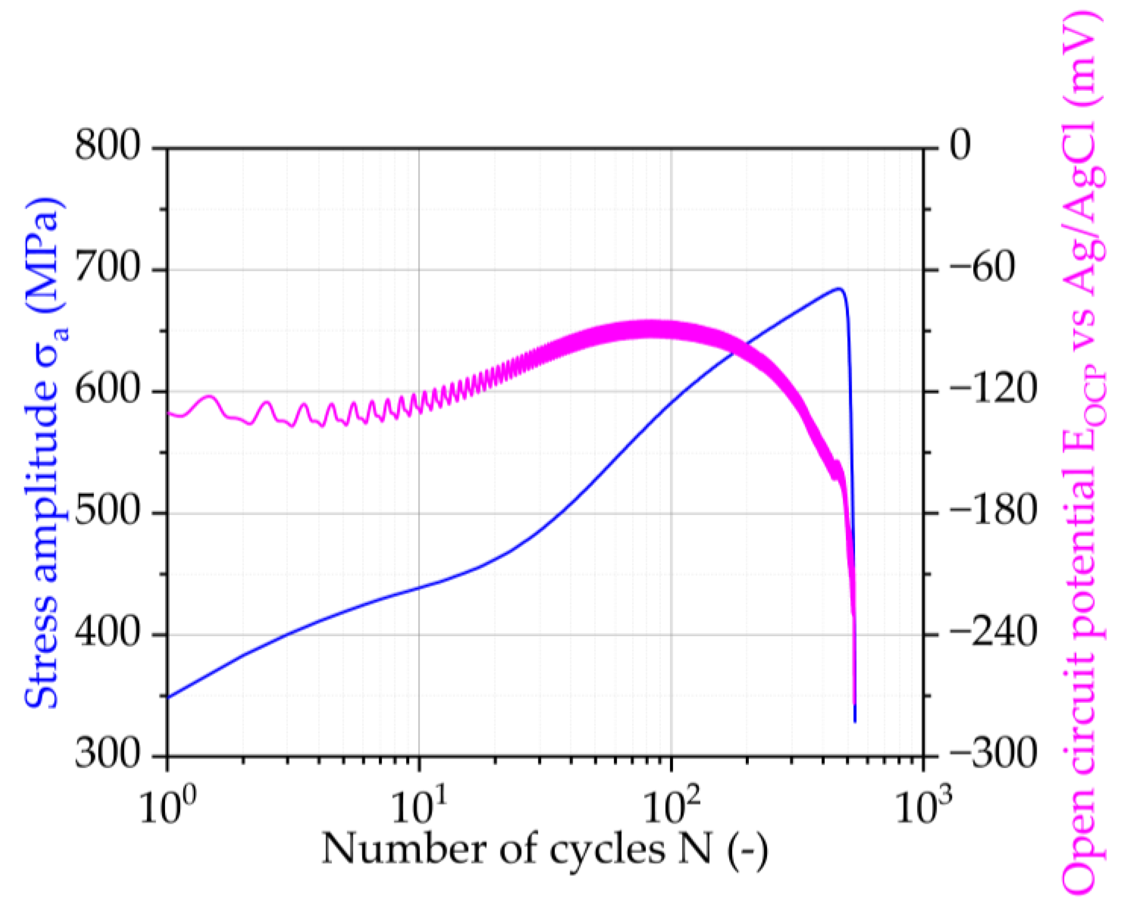
6.3. Electrochemical Potential

To perform measurements of this character the specimen has to be surrounded by an electrolyte. The system is configured on the basis of three electrodes, where the specimen itself serves as one while a graphite electrode serves as an opposing electrode and an Ag/AgCl electrode serves as a reference electrode respectively. The opposing electrode and the reference electrode have been placed to the specimen as close as possible, which allows the open circuit potential to be measured.

Figure 5 shows the result obtained from a CAT under reversed strain-controlled fatigue loading in distilled water, where the open circuit electrical potential E_OCP has been recorded as well as the stress amplitude, showing, that those parameters are independent of the controlling strain and also obey different trends. While the material continuously hardens under cyclic loading, E_OCP shows initially a similar trend, which then obviously changes due to additional reactions resulting between the specimen’s surface and the distilled water surrounding.

6.4. Feritscope

Transformation of metastable austenite to α’-martensite is associated with a change in electromagnetic permeability. A commercial product operating on this basis and in accordance with the DIN EN ISO 2178 standard is a Feritscope [16]. The system consists principally of a solenoid circumference with a coil generating a magnetic field, which results in an induction as soon as paramagnetic martensite is transformed and which is further recorded by a second coil allowing permeability to be measured in a defined region of interest. The instrument used has been a Fischerscope^® MMS.

6.5. Temperature Measurements

Temperature measurements can be used to characterize the fatigue behavior and damage evolution process of metals since the irreversible plastic deformation work is converted by approximately 90 to 95% into heat [17]. This heat is related to the released energy to a lower degree from dislocation movements’ processes, followed significantly from a material’s plasticity generated through an increasing number of slip bands and finally due to crack formation and propagation resulting from stress intensities at the crack tips and possibly also internal friction along crack borders [18].

Temperature measurements were recorded using an IR camera, defining three measuring fields of 10 × 10 pixels each. The main measuring field (T₁) was placed in the center of the specimens’ gauge length and the other two were used as a reference in the upper and lower shafts of the specimen (T₂ and T₃). A temperature difference $\Delta T$ has been determined as a parameter in accordance with the following relationship:

$$\Delta T=T_1-\frac{\left(T_2+T_3\right)}{2}$$

(3)

The result of such a temperature measurement can be seen in Figure 6. It shows that the different strain levels can be clearly recognized. As long as loading is completely elastic, temperature stays fairly constant at each of the levels. However, the increased martensitic transformation during plastic deformation and therefore hardening of the material can be clearly observed as a decrease in temperature.

7. Transferring Materials Data onto Notched Components

7.1. Simulation Results for Unnotched Specimens—The Three-Component Chaboche Plasticity Model

Appropriate understanding of a material’s behavior, specifically also at a microscopic level is a major prerequisite to allow components in service to be assessed appropriately. The more and adequate information that can be obtained, the better an assessment can become. The way to get materials data with an enhanced usage of NDT technology, as presented and discussed above, is therefore an essential element, which even becomes more essential once an aging component has to be assessed.

Assessment of components, pristine as well as aged, is initially to be performed on a numerical basis. For this, an adequate material database is required such that an appropriate description of a material’s behavior can be made based on the mechanical models available. An example in that regard is the three-component Chaboche model [19,20], which claims to describe the nonlinear kinematic hardening of a material. In this model, the displacement of the yield surface of the stress states is described by the back stress tensor α. The temporal changes of the three back stress components ${\alpha }_i$ are linked to the change in plastic strain via model parameters as follows:

$$\dot{{\alpha }_i}=\frac{2}{3}{C}_i{\dot{\epsilon }}^{pl}-{\gamma }_i\left|{\dot{\epsilon }}^{pl}\right|\alpha$$

(4)

The parameters C_i, γ_i, i = 1, 2, 3 are constants in the Chaboche kinematic hardening model, generated from the uniaxial strain controlled stable hysteresis loop.

The uniaxial yield stress ${\sigma }_x$ is the sum of the offset yield stress ${\sigma }_0$ and the back stress component in the uniaxial direction, expressed as:

$${\sigma }_x={\sigma }_0+{\displaystyle \sum }_{i=1}^n{\alpha }_i$$

(5)

These descriptive quantities were determined separately for two selected test temperatures (RT and 240 °C in the present case). To get the parameters determined, stress-strain hystereses of total strain-controlled tests on unnotched specimens are required, preferably performed at different strain amplitudes. The parameters of the material studied were determined on an SIT with an initial ${\epsilon }_{a,t}$ of 0.05% and a step increase of 0.05% performed at RT and 240 °C respectively.

Figure 7a shows the results of the SIT conducted at RT (Specimen NA01). The red line represents the controlled total strain amplitude ${\epsilon }_{a,t}$ and the blue the resulting stress amplitude ${\sigma }_a$. The green line represents the mean stress ${\sigma }_M$, which is a consequence of the strain-controlled mode and the brown the plastic strain amplitude ${\epsilon }_{a,p}$. It can be seen that at lower total strain amplitudes (0.05% to 0.3%), no material hardening or softening does occur, while from 0.35% onwards cyclic hardening is to be seen. Moreover, mean stresses mainly vanish from a total strain amplitude of 0.4% and above. Figure 7b shows the stress-strain hysteresis in the middle of each step. From these hystereses, it was concluded that from ${\epsilon }_{a,t}$ = 0.4% onwards plastic effects are clearly present. Based on this, the step at ${\epsilon }_{a,t}$ = 0.45% (shown in red) was chosen to represent the material under plastic strain and hence for the determination of the parameters in the three-component Chaboche model to be then used in the FE simulations to follow, the cycle used was cycle 9941.

Figure 8 presents the results of a SIT run at 240 °C with the same test parameters as at RT. The respective material responses are presented with the same colors as in Figure 7a. It can be seen, that at the beginning of the test there is a lower mean stress than at RT, which becomes 0 at ${\epsilon }_{a,t}$ = 0.3%. On the other hand, there is a slight softening of the material at lower ${\epsilon }_{a,t}$ from 0.15 to 0.25% and after this point, a slight cyclic hardening is observed in every step. The highest ${\sigma }_a$ reached at elevated temperature is much lower than at RT, due to the absence of martensitic transformation.

Using the materials data presented in Figure 7, the parameters for the Chaboche model were determined for RT (

Table 2. Chaboche parameters for RT, determined using specimen NA01 at cycle 9941.

σ0	C1	γ1	C2	γ2	C3	γ3
122	2,000,000	77,300	130,000	560	15,200	3340

) and a hysteresis was simulated and compared with measured data as shown in Figure 9, where a good coincidence is to be seen.

The same was also done for 240 °C (

Table 3. Chaboche parameters for 240 °C, determined at load cycle 8000.

σ0	C1	γ1	C2	γ2	C3	γ3
47.6	2,098,000	137,000	651,000	17,300	84,400	4.99

), and the validated results are shown in Figure 10. Parameters were determined for a total strain amplitude of 0.25%.

With this it is shown, that SITs can provide an interesting basis, to get parameters for the Chaboche model determined at very short term and this even in accordance with a material’s degree of degradation.

7.2. Simulation of Material’s Behavior in Notched Components

A question arises when a notch is fairly small and sharp and when the local stresses and strains in the notch root cannot be determined experimentally: Can the stresses and strains in the notch root be appropriately determined through numerical simulation? The type of notched specimen shown in Figure 1, being a round bar specimen with a circumferential grooved notch of R_N = 0.35 and 0.5 mm in notch radius respectively, loaded under axial loading, has been analyzed experimentally as well as numerically. Results obtained from the respective fatigue tests conducted as a LIT at RT (Specimen 14.7) are presented in Figure 11a and an SIT at RT (Specimen 14.3) in Figure 11b. Since neither stresses nor strains could be measured locally, the stresses and strains are considered as nominal stress $S$ (load divided by minimum cross-section) and nominal strain $e$ (deflection divided by an 8 mm gauge length) respectively. It can be seen that significant plastic deformation occurs in the minimum cross-section of the specimen and that the notch is shortly facing a full plastic environment.

The results shown in Figure 11 have been used to validate the numerical approach based on the Chaboche model, as described before. The comparison was done on the basis of nominal strains (hence the measured deflections). In general, there are differences between calculations with different Chaboche parameter sets. Therefore, a statement on the validity of the notch-based predictions is necessary. The results obtained are shown in Figure 12. A difficulty arises in a way that the material used has shown strong softening and possibly also hardening effects. Those effects are to be seen as a variation in mean strain in load-controlled tests such as the LIT considered here. These changes do also have an influence on the parameters for the Chaboche model considered in the numerical simulation. However, in the numerical simulation presented here, only some average parameters for the Chaboche model could be considered. To avoid those changes and allow for adequate comparability, those softening and hardening effects have been removed in the first instance and have been indicated as ‘centered’ in Figure 12 respectively. This correlation is valid up to the validity of the plasticity model, which is considered to be the level at which the Chaboche parametrization was done, in this case at 0.45% maximum strain. Principally this approach could be extended in a way that the parameters for the Chaboche model could be determined for the different softening and hardening conditions. Even the creep-like mean stress effects could be described more appropriately.

With the numerical simulation being available, strains in the notch root can be determined. Those strains have been plotted versus the nominal strains, where the result is shown in Figure 13. Following Neuber’s Equation (6), which can be simply written as

$$K_t^2=K_{\sigma }·K_{\epsilon }$$

(6)

the strain concentration factor $K_{\epsilon }$ can now be determined, which is nothing else than

$$K_{\epsilon }=\frac{strain in notch root}{nominal strain}=\frac{{\epsilon }_N}{e}$$

(7)

As can be seen from the results in Figure 13, $K_{\epsilon }$ clearly depends on the load being applied. In a similar way also the stress concentration factor $K_{\sigma }$ could be determined.

With this, it also becomes clear that the high strain in the notch root partly exceeds the strain level of the hysteresis used for calibration after step 5 of the nominal LIT with the parameters described before. At these load levels, the differences between the individual parameters are sometimes very large. Within the scope of validity, the parameter sets calculated with the results of specimen NA01, cycle 9941 show very good agreement.

The relationship shown as an example in Figure 13 may also be described analytically. In that case, an odd third degree polynomial may fit the data using Equation (8) for R_N = 0.35 mm, and Equation (9) for R_N = 0.5 mm respectively.

$${\epsilon }_{a,t,N}=4.11·e_{a,t;8}+130.86·e_{a,t;8}^3$$

(8)

$${\epsilon }_{a,t,N}=3.67·e_{a,t;8}+50.6·e_{a,t;8}^3$$

(9)

Since the behavior in a notch root fully defines the behavior of a notched component, it becomes essential to describe what is happening in a notch root. For this, concepts like the local strain approach have been developed, having been widely described in the literature. A crucial part of those concepts is the nominal stress versus the notch strain relationship, where Neuber’s equation [21] mentioned before is now formulated as

$$S^2·K_t^2=\frac{\sigma ·\epsilon }{E}$$

(10)

with $S$ representing nominal stress, $K_t$ the so-called stress concentration factor (which is truly a function of stress and strain concentration, as to the equation above), $E$ Young’s modulus and $\sigma$ and $\epsilon$ the local stress and strain in the notch root respectively. If $S$ is known from the load applied and $K_t$ obtained from handbooks, numerical simulations or measurements, then the remaining unknowns $\sigma$ and $\epsilon$ describing the material’s constitutive behavior can be determined by including such a relationship as described by the Ramberg-Osgood relationship

$$\epsilon ={\epsilon }_e+{\epsilon }_{p }=\frac{\sigma }{E}+{\left(\frac{\sigma }{K^{\prime }}\right)}^{\raisebox{1ex}{$1$}\!\left/ \!\raisebox{-1ex}{$n^{\prime }$}\right.}$$

(11)

or others, where ${\epsilon }_e$ and ${\epsilon }_p$ describe the elastic and plastic portion of strain and $K\prime$ and $n\prime$ represent a coefficient and an exponent describing the material’s plastic behavior respectively.

Strictly speaking, Neuber’s equation is only valid for purely elastic material behavior, but it is also applicable if the plastic zones in a notch are small compared to the component size. If the plastic zones become large, i.e., the fully plastic limit load of a component is reached, Neuber’s equation increasingly overestimates the notch root stresses, which has led to a modification of the equation as proposed by Seeger and Beste [22].

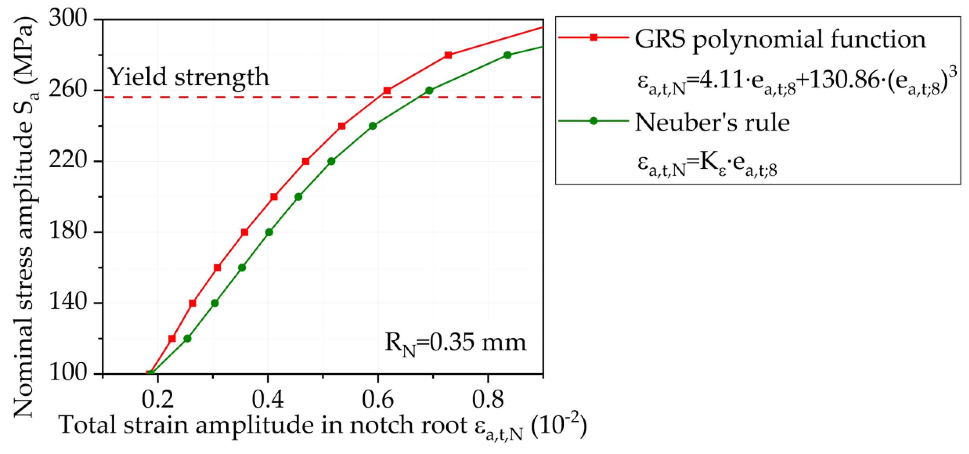
Figure 14 shows the comparison of the numerically calculated notch root strains for the specimen with a notch radius of R_N = 0.35 mm for an SIT performed at RT, where the considered gauge length of the deformation transducer was 8 mm. The values marked in red were determined via the polynomial function derived from FEM calculations. The range of validity of this function extends over total strain amplitudes up to ~0.45%, allowing nominal stress amplitudes of up to $S_a$ = 200 MPa to be considered. The green curve was obtained using $K_{\epsilon }$ and Neuber’s equation in the form presented in Equation (7). It can be observed that the notch strains determined analytically are higher than those determined by FEM. Figure 15 shows the same comparison as described above, but now for the specimen with R_N = 0.50 mm.

8. Conclusions

The assessment of the integrity of engineering structures is a complex task, which needs a deeper look into the materials degradation processes before a crack in the material or structure appears. For this purpose, the use of different NDT techniques presents a great advantage, being able to monitor the materials’ response and collect materials data when exposed to a mechanical or electromagnetic wave, without causing any extra degradation on the material or structure.

In nuclear power plants, structures are subjected to high temperature transients and harsh environmental conditions and the consequences of structural failure are known to be dramatic. High safety factors have therefore been imposed on those structures, to get failure avoided. On the other hand, those structures would have a residual life potential left when modern technology, not having been available at the time of those structures’ design, would have been included. This inclusion could be seen as an invaluable benefit, in case a structure’s life extension could be considered. Advanced inspection technology, a better understanding of materials’ microstructure as well as behavior, and the option of numerically mimicking the observed phenomena in a prognostic way is far beyond what has been the basis of assumptions having been made in design in the past. This also includes strategies for the replacement of certain parts after an established period of time and may impact design codes and standards. A further economic impact is to be seen by better taking advantage of an infrastructure’s potential in general, and in the specific case here the extension of the operational life of nuclear power plants.

Assessments of aged materials and structures with respect to their residual fatigue life is a task to be performed relatively quickly and at minimum cost. Furthermore, the availability of adequate material is often highly limited in that case. Generation of S-N curves based on twenty to thirty fatigue tests to be performed—and this even under different environmental conditions—is a close to impossible scenario. As such it becomes clear, that a method to evaluate the S-N curves in a short period is in need. The STEPs for the enhanced evaluation of fatigue data play here an important role, making it possible to generate an S-N curve with three specimens only.

The provision of adequate materials information is a prerequisite for an adequate numerical simulation. Enhanced computation power and an increasing number of sophisticated numerical models allow conditions to be simulated today, which were impossible to simulate at the time when most of our current infrastructure has been designed and realized. This also applies to nuclear power plants. These numerical simulation tools are merged in the meantime with increasingly growing databases, that result in what is defined as digital twins. These can be principally established for any type of structure, would it be aged or new.

MibaLeb does not claim to provide digital twins for nuclear engineering applications. However, what it claims is to provide appropriate materials information, that can be fed into such digital twins in the longer term. Getting such digital twins established is a tremendous task, possibly living as long as the respective infrastructure’s life and possibly beyond. In MibaLeb this digital twin’s related activity has been limited to the provision of materials data and information related to AISI 347 (X6CrNiNb18-10) exposed to a series of hot and cold water flow conditions, and validated as an example on a pressurized hot water pipe segment. MibaLeb has laid a foundation on how such a digital twin could be built up and how it could be fed with data. Since this digital twin development is a living job with a most likely open end, there are still further questions that emerge and that need to be answered in the future, such as:

• STEPs for the evaluation of fatigue data: Can reliable scatter bands be generated using STEPs? Is the use of STEPs only valid for HCF or could these methods be extended to be used in the LCF and VHCF regimes?
• NDT techniques to assess material’s degradation: After understanding the materials degradation process of the AISI 347 under different loading and environmental conditions using destructive testing methods and microstructural investigations, which NDT method or any combination of those may best reflect each degradation process? Would the limitations of a single NDT method be overcome by a combination of different methods?
• Numerical modeling of structures: Can the data generated by STEPs and NDT methods be used to generate a numerical model (digital twin) of the structure being capable of assessing the residual lifetime of the modeled structure? What are the limitations of those models? How could the materials’ related aspects brought in by MibaLeb be merged with further structural aspects such as structural dynamics, stability, fluid-structure interaction and possibly others in the sense of a digital twin?

Even though it appears to be a long way to go before these concepts can be adopted in international standards, the MibaLeb project is making its big contribution in putting all those concepts together, using the expertise of different academic and non-academic institutions in each of the competent fields. It has opened a field that is far from having been completed so far. However, if the approach taken can be proven at this relatively generic level, a next step can follow, where the complexity of the approach will be increased. In the current case a next step will be to predict S-N curves for pipes and to get those predictions reflected with past design data as well as with real results. This could be followed by the inclusion of a different material, possibly one which is exposed to irradiation, which would bring in an additional environmental parameter and possibly additional damage mechanisms. The concept is hence adaptable to further extensions.