
Novel Modelling Approach for Obtaining the Parameters of Low Ionosphere under Extreme Radiation in X-Spectral Range

 ,
,  , and
, and
Abstract
:1. Introduction
2. SFs Impact
2.1. Monitoring SF
2.2. Used Numerical Methods
2.2.1. Two-Component Exponential Model and Simulations
2.2.2. FlarED’ Method
2.2.3. Approximate Analytic Expression
3. Results and Discussion
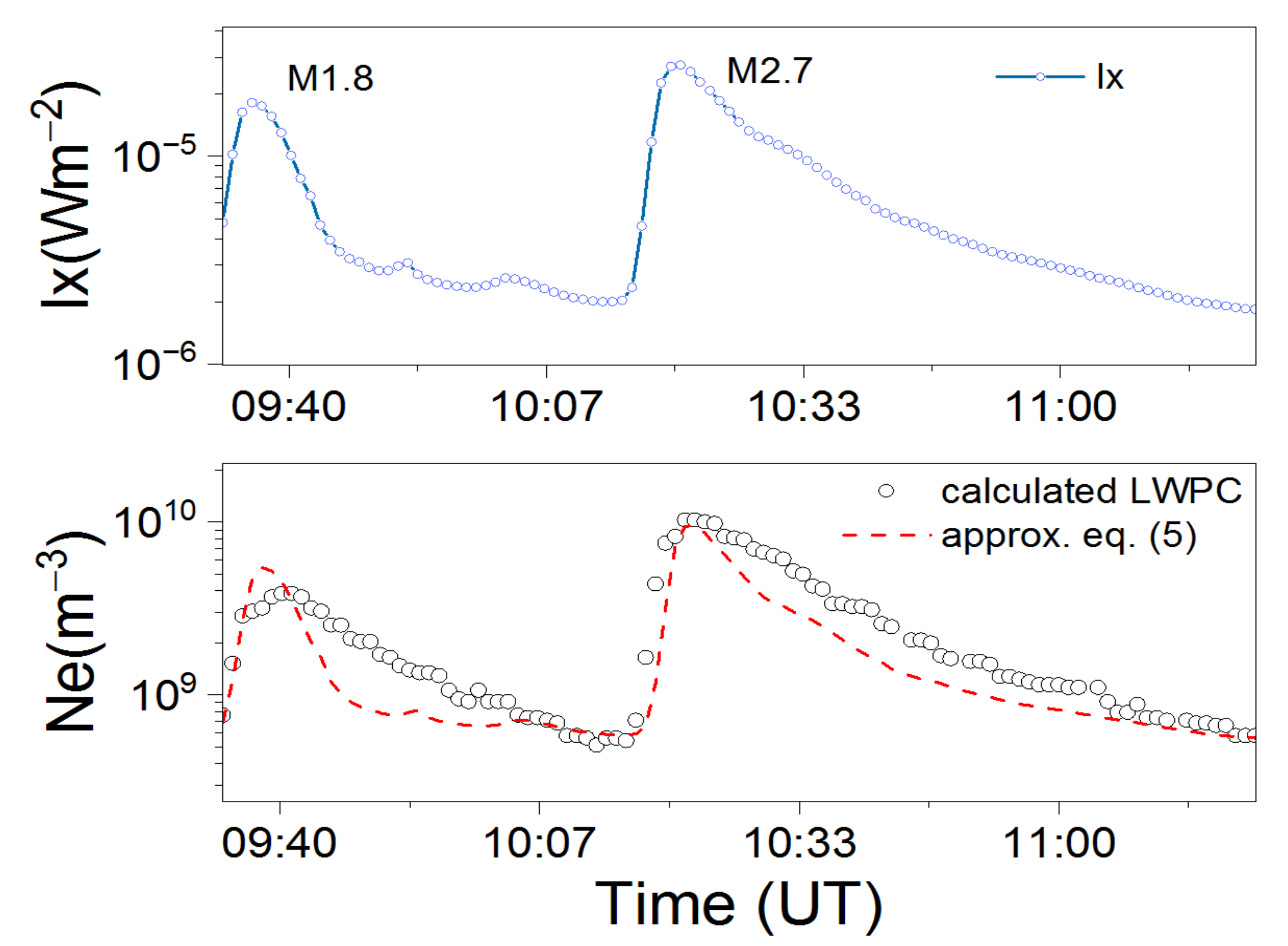
3.1. Analyses of SF Events
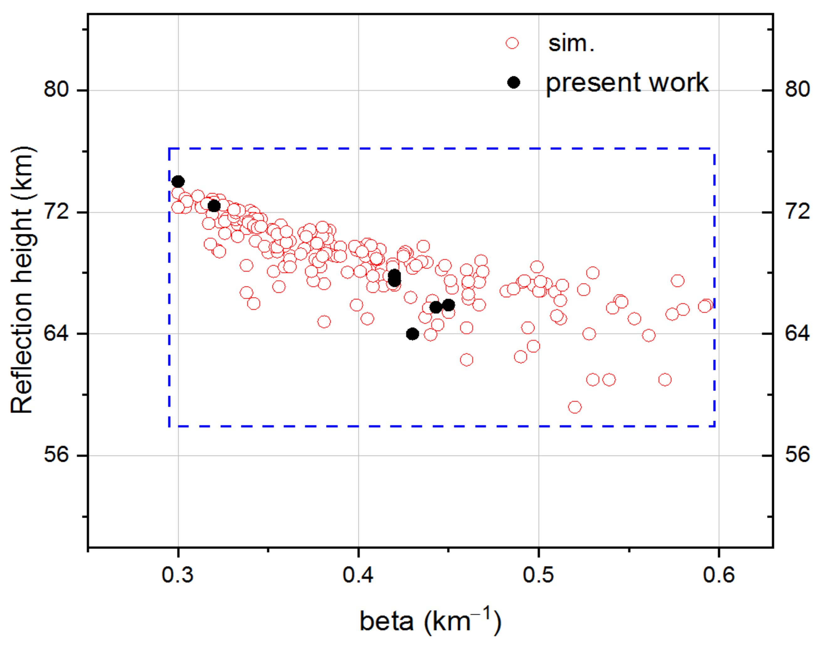
3.2. Approximative Expressions and Simulations
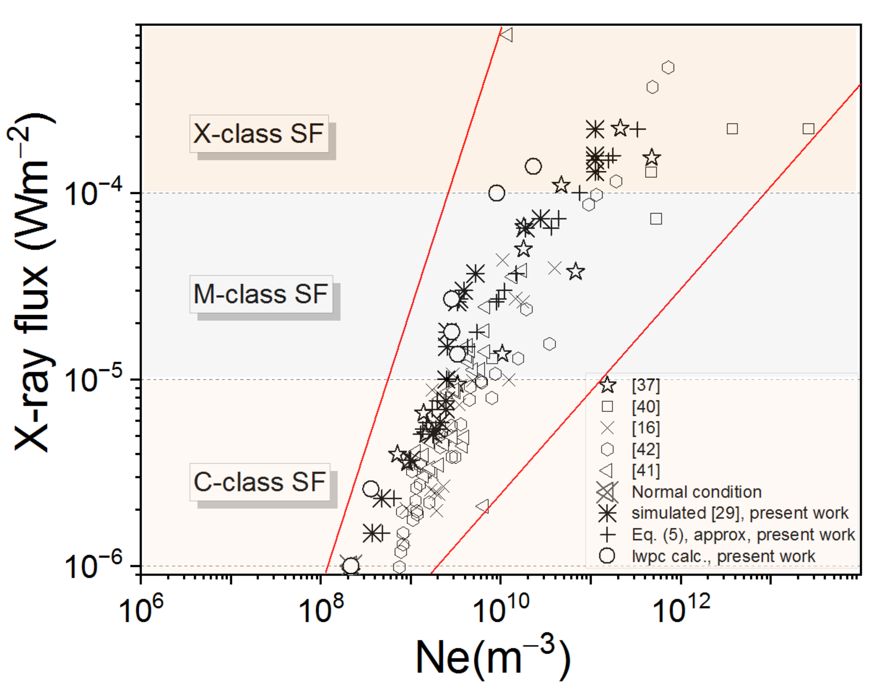
3.3. Comparison of Results
4. Conclusions and Perspectives
Author Contributions
Funding
Institutional Review Board Statement
Informed Consent Statement
Data Availability Statement
Acknowledgments
Conflicts of Interest
References
- Bothmer, V.; Daglis, I.A. Space Weather: Physics and Effects; Springer Science & Business Media: Berlin/Heidelberg, Germany, 2007. [Google Scholar]
- Smith, H.J.; Smith, E.V.P. Solar Flares; Macmillan: New York, NY, USA, 1963. [Google Scholar]
- Davidson, B. Weatherman’s Guide to the Sun, 3rd ed.; Space Weather News, LLC.: New York, NY, USA, 2020. [Google Scholar]
- Doschek, G.; Meekins, J.; Cowan, R.D. Spectra of solar flares from 8.5 Å to 16 Å. Sol. Phys. 1973, 29, 125–141. [Google Scholar] [CrossRef]
- Tandberg-Hanssen, E.; Emslie, A.G. The Physics of Solar Flares; Cambridge University Press: Cambridge, UK, 2009. [Google Scholar]
- Reames, D.V.; Murdin, P. Solar Wind: Energetic Particles. Encycl. Astron. Astrophys. 2002, 2312, 1–122. [Google Scholar]
- Tandon, J.; Deshpande, S.; Bhatia, V. Electromagnetic radiation from solar flares. Nature 1968, 220, 1213–1214. [Google Scholar] [CrossRef]
- Brasseur, G.P.; Solomon, S. Composition and chemistry. In Aeronomy of the Middle Atmosphere: Chemistry and Physics of the Stratosphere and Mesosphere; Springer: Berlin/Heidelberg, Germany, 2005; pp. 265–442. [Google Scholar]
- Nina, A.; Čadež, V.; Srećković, V.; Šulić, D. The influence of solar spectral lines on electron concentration in terrestrial ionosphere. Open Astron. 2011, 20, 609–612. [Google Scholar] [CrossRef] [Green Version]
- Valnicek, B.; Ranzinger, P. X-ray emission and D-region “sluggishness”. Bull. Astron. Inst. Czechoslov. 1972, 23, 318. [Google Scholar]
- Bain, W.C.; Hammond, E. Ionospheric solar flare effect observations. J. Atmos. Sol. Terr. Phys. 1975, 37, 573–574. [Google Scholar] [CrossRef]
- Brasseur, G.P.; Solomon, S. Radiation. In Aeronomy of the Middle Atmosphere: Chemistry and Physics of the Stratosphere and Mesosphere; Springer: Berlin/Heidelberg, Germany, 2005; pp. 151–264. [Google Scholar]
- Mitra, A.P. Ionospheric Effects of Solar Flares; Springer: Berlin/Heidelberg, The Netherlands, 1974. [Google Scholar] [CrossRef]
- Nicolet, M.; Swider, W., Jr. Ionospheric conditions. Planet. Space Sci. 1963, 11, 1459–1482. [Google Scholar] [CrossRef]
- Garcia, H.A. Temperature and emission measure from GOES soft X-ray measurements. Sol. Phys. 1994, 154, 275–308. [Google Scholar] [CrossRef]
- Grubor, D.; Šulić, D.; Žigman, V. Classification of X-ray solar flares regarding their effects on the lower ionosphere electron density profile. Ann. Geophys. 2008, 26, 1731–1740. [Google Scholar] [CrossRef] [Green Version]
- Wang, X.; Chen, Y.; Toth, G.; Manchester, W.B.; Gombosi, T.I.; Hero, A.O.; Jiao, Z.; Sun, H.; Jin, M.; Liu, Y. Predicting solar flares with machine learning: Investigating solar cycle dependence. Astrophys. J. 2020, 895, 3. [Google Scholar] [CrossRef]
- Kelley, M.C. The Earth’s Ionosphere: Plasma Physics and Electrodynamics, ser. International Geophysics, 2nd ed.; Academic Press: Cambridge, MA, USA, 2009. [Google Scholar]
- Wah, W.P.; Abdullah, M.; Hasbi, A.M.; Bahari, S.A. Development of a VLF receiver system for sudden ionospheric disturbances (SID) detection. In Proceedings of the 2012 IEEE Asia-Pacific Conference on Applied Electromagnetics (APACE), Melaka, Malaysia, 11–13 December; pp. 98–103.
- Šulić, D.; Srećković, V.; Mihajlov, A. A study of VLF signals variations associated with the changes of ionization level in the D-region in consequence of solar conditions. Adv. Space Res. 2016, 57, 1029–1043. [Google Scholar] [CrossRef] [Green Version]
- Volland, H. On the solar flare effect of vlf-waves in the lower ionosphere. J. Atmos. Sol.-Terr. Phys. 1964, 26, 695–709. [Google Scholar] [CrossRef]
- Šulić, D.; Srećković, V. A comparative study of measured amplitude and phase perturbations of VLF and LF radio signals induced by solar flares. Serb. Astron. J. 2014, 188, 45–54. [Google Scholar] [CrossRef] [Green Version]
- Ferguson, A.J. Computer Programs for Assessment of Long-Wavelength Radio Communications, Version 2.0: User’s Guide and Source Files; Space and Naval Warfare Systems Center: San Diego, CA, USA, 1998. [Google Scholar]
- LWPC. Computer Programs for Assessment of Long-Wavelength Radio Communications, V2.1. 2018. Available online: https://github.com/space-physics/LWPC (accessed on 30 June 2021).
- Nina, A.; Čadež, V.; Srećković, V.; Šulić, D. Altitude distribution of electron concentration in ionospheric D-region in presence of time-varying solar radiation flux. Nucl. Instrum. Methods Phys. Res. B 2012, 279, 110–113. [Google Scholar] [CrossRef] [Green Version]
- Nina, A.; Čadež, V.; Šulić, D.; Srećković, V.; Žigman, V. Effective electron recombination coefficient in ionospheric D-region during the relaxation regime after solar flare from February 18, 2011. Nucl. Instrum. Methods Phys. Res. B 2012, 279, 106–109. [Google Scholar] [CrossRef] [Green Version]
- Žigman, V.; Grubor, D.; Šulić, D. D-region electron density evaluated from VLF amplitude time delay during X-ray solar flares. J. Atmos. Sol.-Terr. Phys. 2007, 69, 775–792. [Google Scholar] [CrossRef]
- Wait, J.R.; Spies, K.P. Characteristics of the Earth-Ionosphere Waveguide for VLF Radio Waves, Technical Note 300; US Department of Commerce, National Bureau of Standards: Boulder, CO, USA, 1964.
- Vujčić, V.; Srećković, V.A. flarED Flare Electron Density. Available online: https://github.com/sambolino/flarED (accessed on 19 September 2021).
- Da Silva, C.L.; Salazar, S.D.; Brum, C.G.; Terra, P. Survey of electron density changes in the daytime ionosphere over the Arecibo observatory due to lightning and solar flares. Sci. Rep. 2021, 11, 1–12. [Google Scholar] [CrossRef]
- Kolarski, A.; Grubor, D. Sensing the Earth’s low ionosphere during solar flares using VLF signals and goes solar X-ray data. Adv. Space Res. 2014, 53, 1595–1602. [Google Scholar] [CrossRef] [Green Version]
- Kolarski, A.; Grubor, D. Comparative analysis of VLF signal variation along trajectory induced by X-ray solar flares. J. Astrophys. Astron. 2015, 36, 565–579. [Google Scholar] [CrossRef]
- Nina, A.; Nico, G.; Mitrović, S.T.; Čadež, V.M.; Milošević, I.R.; Radovanović, M.; Popović, L.Č. Quiet Ionospheric D-Region (QIonDR) Model Based on VLF/LF Observations. Remote Sens. 2021, 13, 483. [Google Scholar] [CrossRef]
- Palit, S.; Basak, T.; Mondal, S.; Pal, S.; Chakrabarti, S. Modeling of very low frequency (VLF) radio wave signal profile due to solar flares using the GEANT4 Monte Carlo simulation coupled with ionospheric chemistry. Atmos. Chem. Phys. 2013, 13, 9159–9168. [Google Scholar] [CrossRef] [Green Version]
- Sezen, U.; Gulyaeva, T.L.; Arikan, F. Online international reference ionosphere extended to plasmasphere (IRI-Plas) model. In Proceedings of the 2017 XXXIInd General Assembly and Scientific Symposium of the International Union of Radio Science (URSI GASS), Montreal, QC, Canada, 19–26 August 2017; pp. 1–4. [Google Scholar]
- Bilitza, D.; Altadill, D.; Truhlik, V.; Shubin, V.; Galkin, I.; Reinisch, B.; Huang, X. International Reference Ionosphere 2016: From Ionospheric Climate to Real-Time Weather Predictions. Space Weather. 2017, 15, 418–429. [Google Scholar] [CrossRef]
- Srećković, V.A.; Šulić, D.M.; Ignjatović, L.; Vujčić, V. Low Ionosphere under Influence of Strong Solar Radiation: Diagnostics and Modeling. Appl. Sci. 2021, 11, 7194. [Google Scholar] [CrossRef]
- Hayes, L.A.; O’Hara, O.S.; Murray, S.A.; Gallagher, P.T. Solar Flare Effects on the Earth’s Lower Ionosphere. Sol. Phys. 2021, 296, 1–17. [Google Scholar] [CrossRef]
- Basak, T.; Chakrabarti, S.K. Effective recombination coefficient and solar zenith angle effects on low-latitude D-region ionosphere evaluated from VLF signal amplitude and its time delay during X-ray solar flares. Astrophys. Space Sci. 2013, 348, 315–326. [Google Scholar] [CrossRef] [Green Version]
- Gavrilov, B.; Ermak, V.; Lyakhov, A.; Poklad, Y.V.; Rybakov, V.; Ryakhovsky, I. Reconstruction of the Parameters of the Lower Midlatitude Ionosphere in M-and X-Class Solar Flares. Geomagn. Aeron. 2020, 60, 747–753. [Google Scholar] [CrossRef]
- Pandey, U.; Singh, B.; Singh, O.; Saraswat, V. Solar flare induced ionospheric D-region perturbation as observed at a low latitude station Agra, India. Astrophys. Space Sci. 2015, 357, 1–11. [Google Scholar] [CrossRef]
- Thomson, N.R.; Clilverd, M.A. Solar flare induced ionospheric D-region enhancements from VLF amplitude observations. J. Atmos. Sol.-Terr. Phys. 2001, 63, 1729–1737. [Google Scholar] [CrossRef]
- Avakyan, S. Supramolecular physics of the solar-troposphere links: Control of the cloud cover by solar flares and geomagnetic storms. In Proceedings of the 11th Intl School and Conference “Problems of Geocosmos”, St. Petersburg, Russia, 3–7 October 2016; pp. 187–191. [Google Scholar]
- Goncharenko, Y.V.; Kivva, F. Evaluation of Size of the Atmospheric Aerosol Particles in the Reflecting Layers Occurring after Intense Solar Flares. Telecommun. Radio Eng. 2003, 59, 1–6. [Google Scholar]
- McGrath-Spangler, E.L.; Denning, A.S. Global seasonal variations of midday planetary boundary layer depth from CALIPSO space-borne LIDAR. J. Geophys. Res. 2013, 118, 1226–1233. [Google Scholar] [CrossRef]
- Mallios, S.A.; Daskalopoulou, V.; Amiridis, V. Orientation of non spherical prolate dust particles moving vertically in the Earth’s atmosphere. J. Aerosol. Sci. 2021, 151, 105657. [Google Scholar] [CrossRef]


| SF Tim | SID VLF Signatures | SF Data | ||||||
|---|---|---|---|---|---|---|---|---|
| SF (Class, Date) | Start [UT] | Peak [UT] | End [UT] | ΔA [dB] | ΔP [deg] | Δt [min] | Ix max XL [Wm−2] | Active Region |
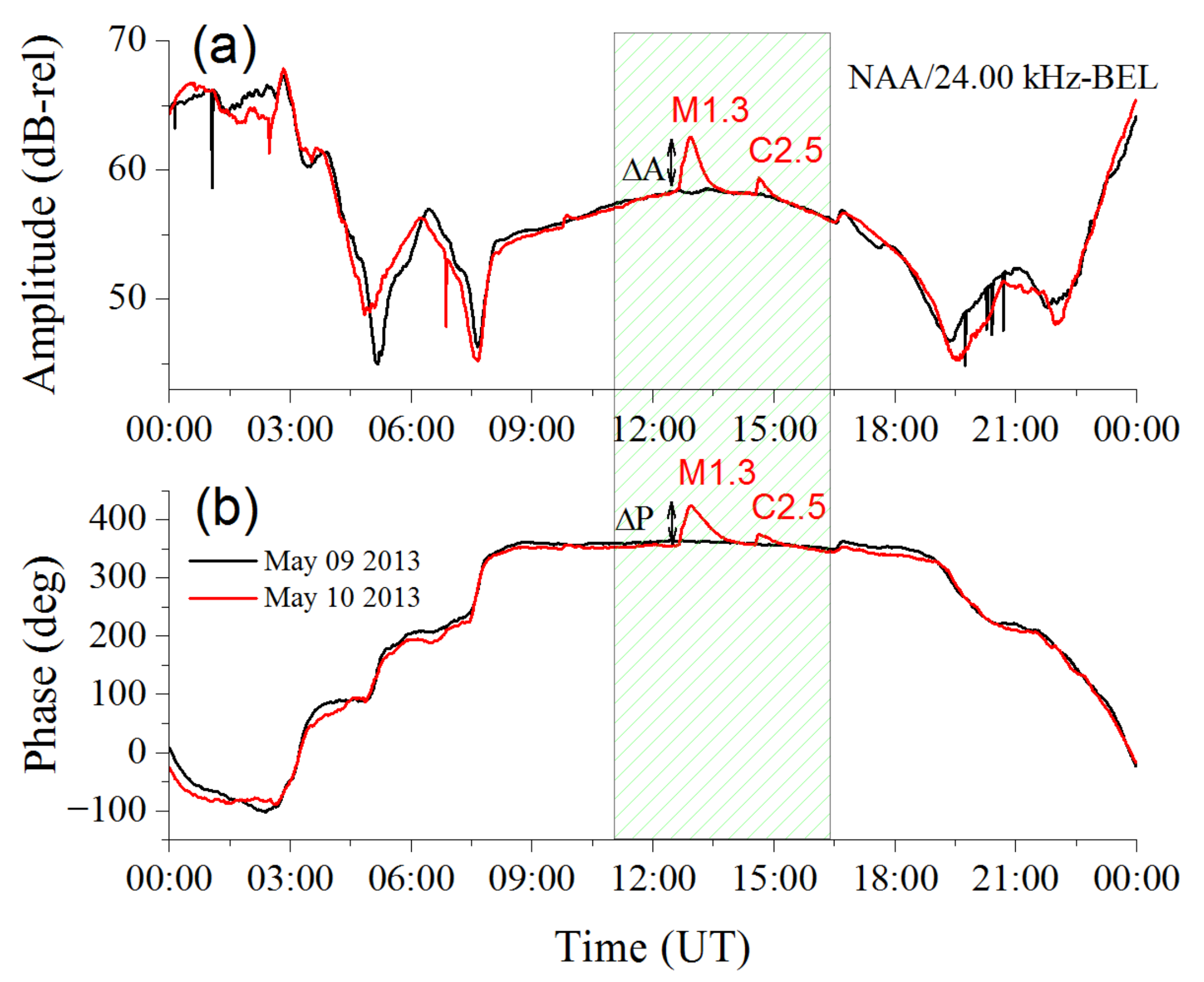
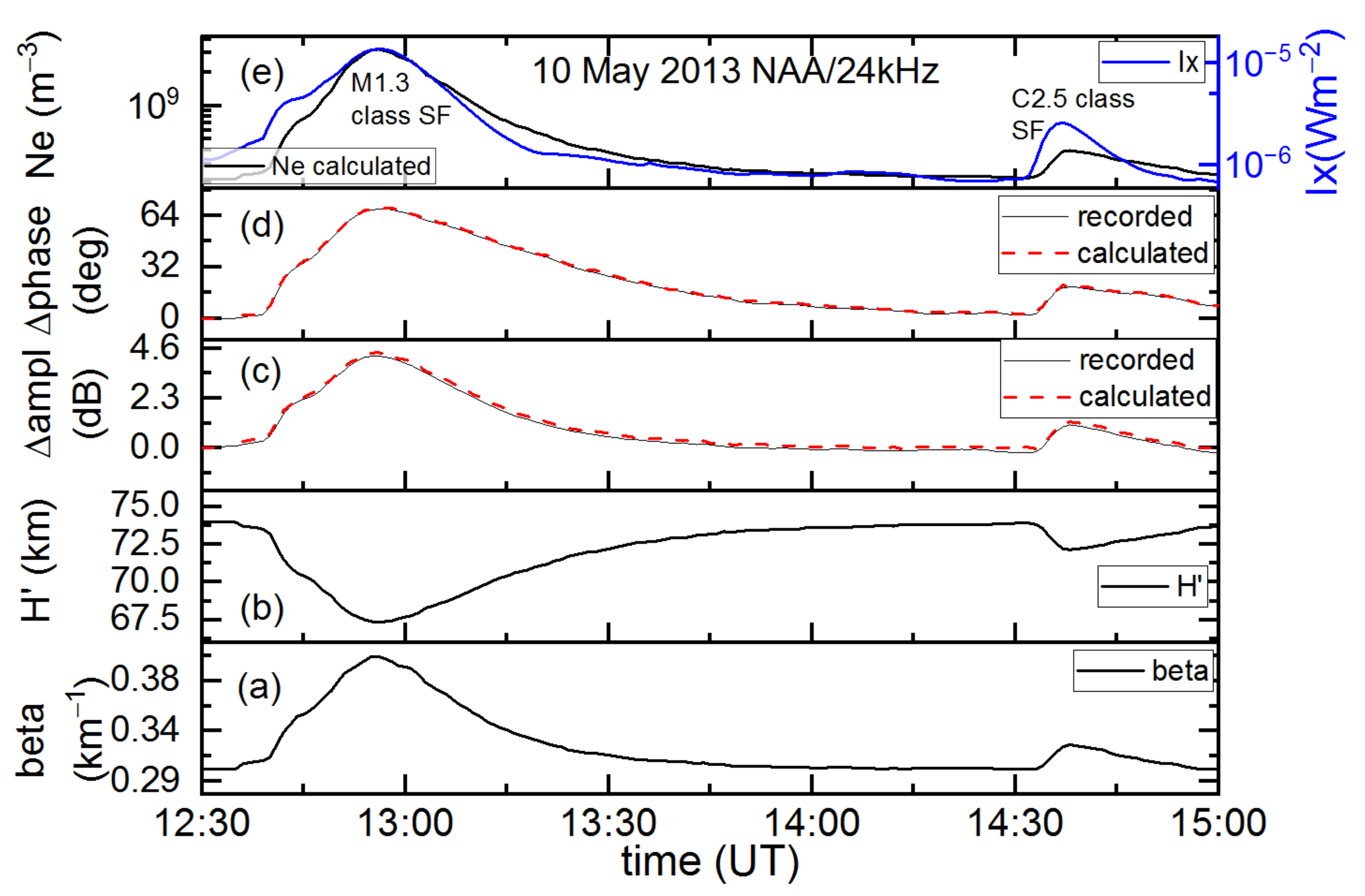
| M1.3 10.05.2013 | 12:37 | 12:56 | 13:04 | 4.20 | 68.19 | 0 | 1.36 × 10⁻⁵ | 1745 |
| C2.5 10.05.2013 | 14:30 | 14:37 | 14:42 | 1.06 | 19.20 | 1 | 2.59 × 10⁻⁶ | 1745 |
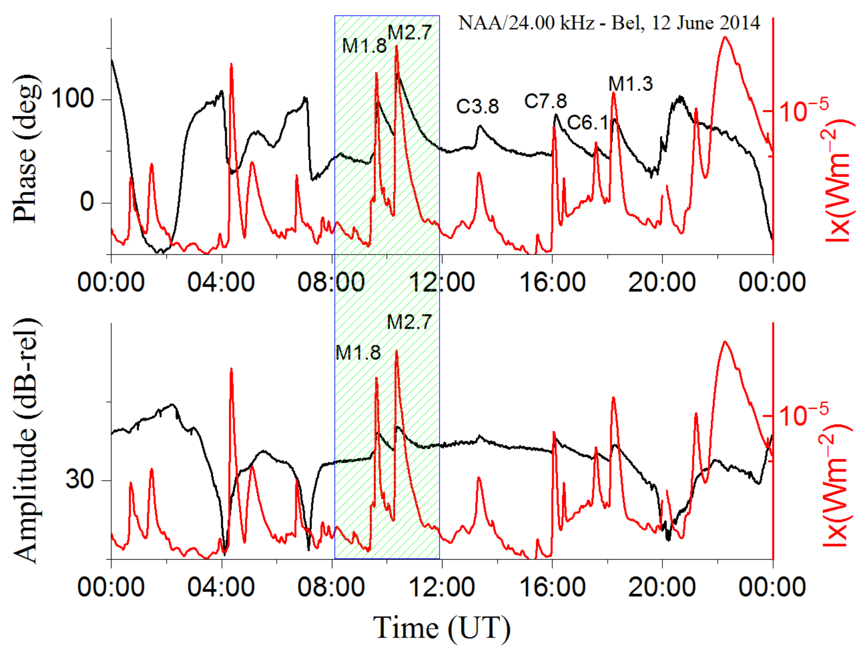
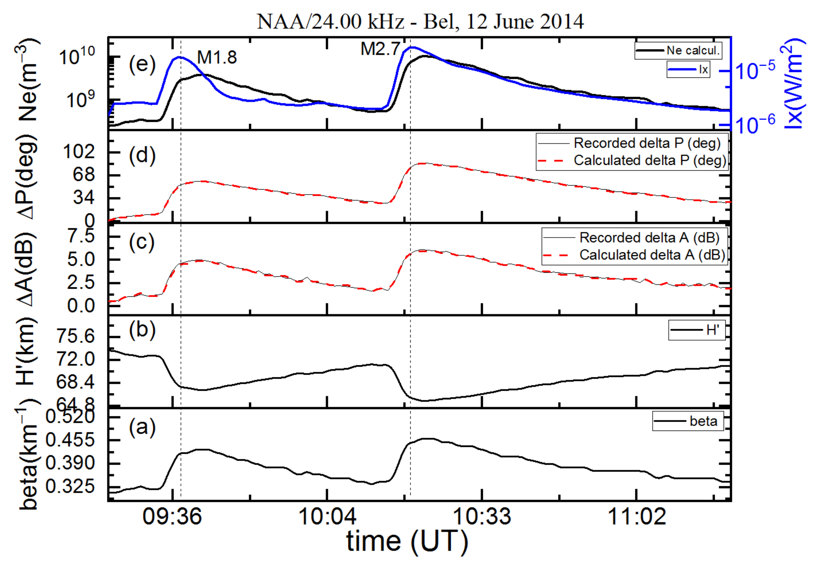
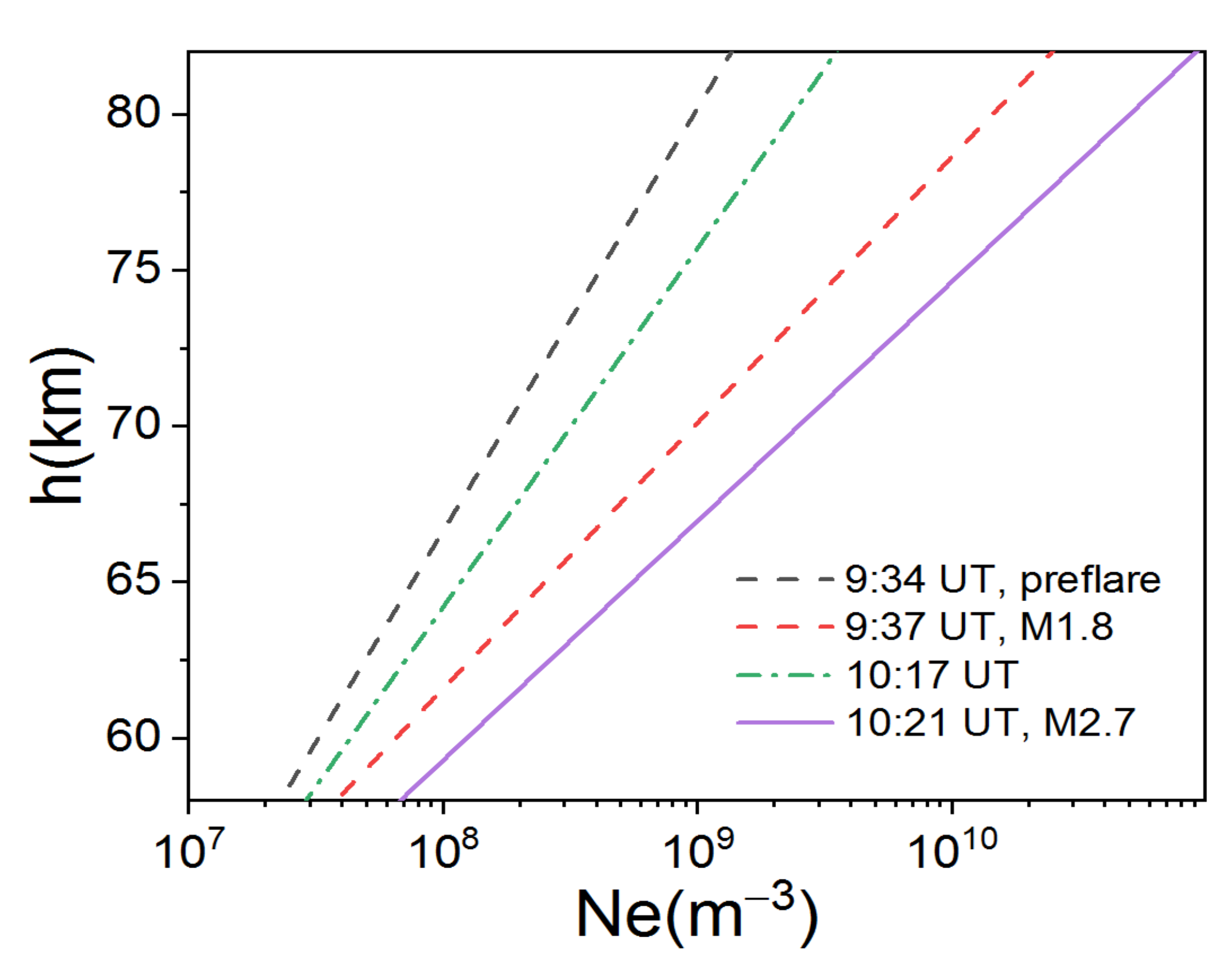
| M1.8 12.06.2014 | 09:23 | 09:37 | 09:42 | 4.50 | 51.47 | 4 | 1.81 × 10⁻⁵ | 2085 |
| M2.7 12.06.2014 | 10:14 | 10:21 | 10:27 | 5.72 | 83.01 | 2 | 2.74 × 10⁻⁵ | 2087 |
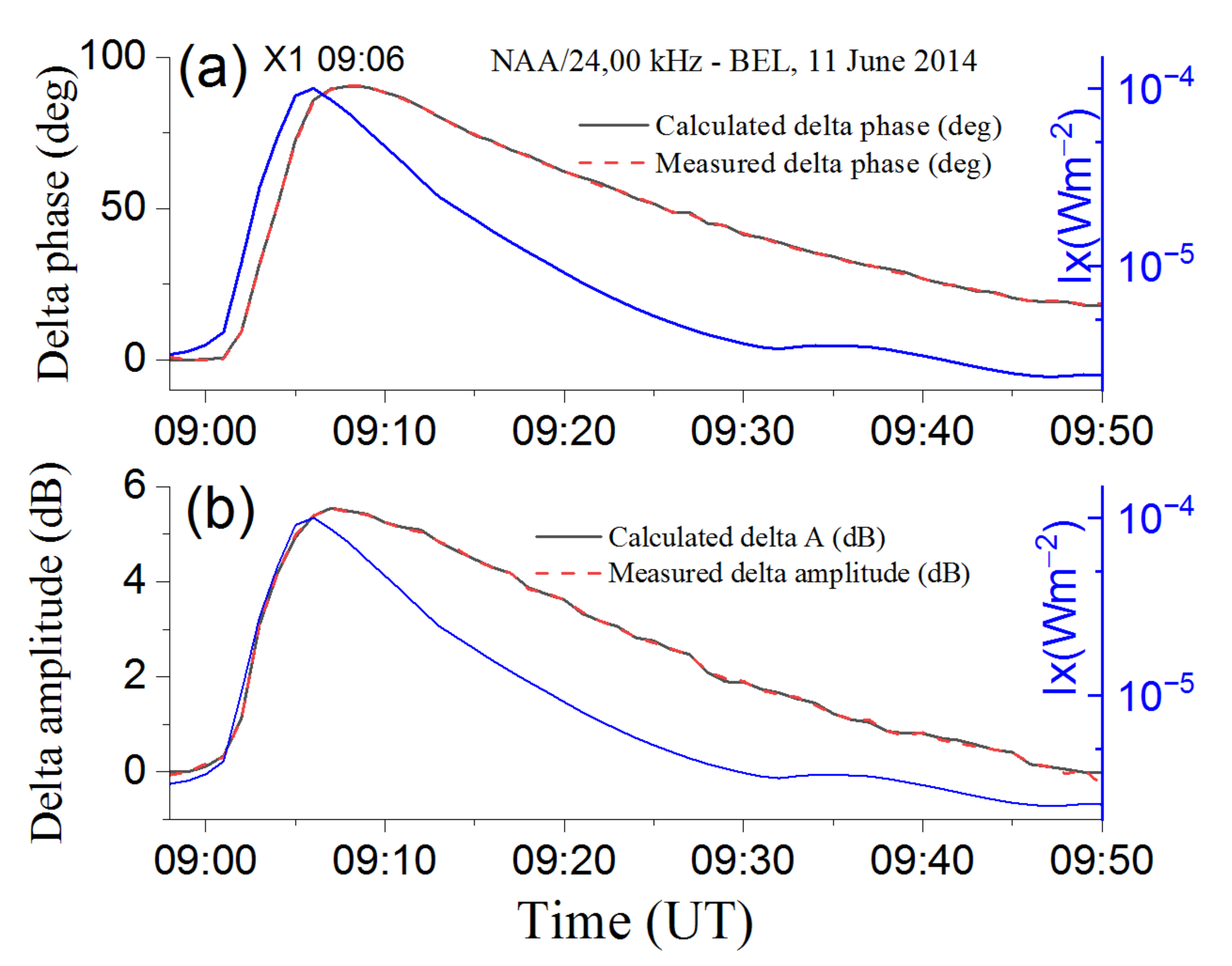
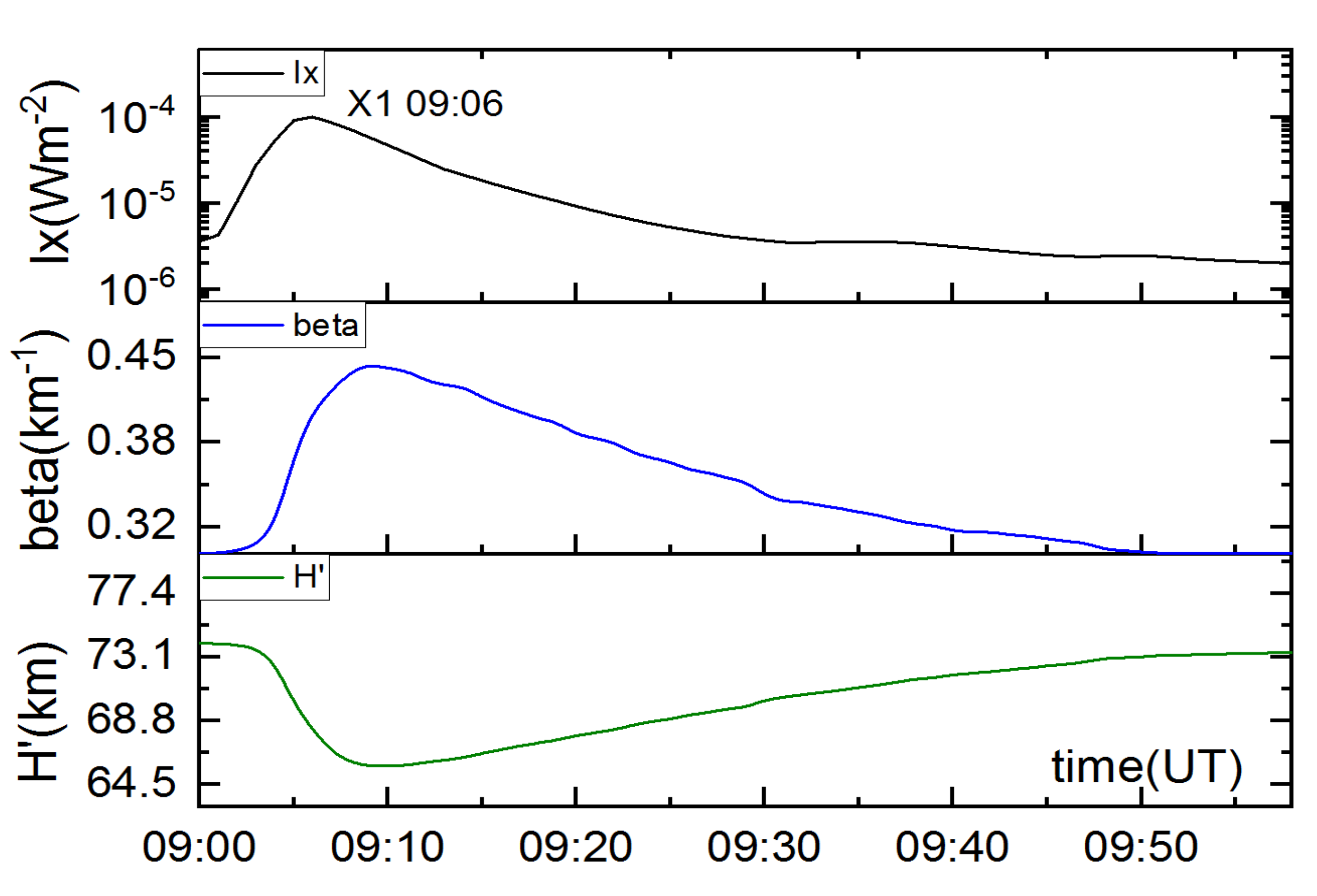
| X1.0 11.06.2014 | 08:59 | 09:06 | 09:10 | 5.54 | 90.45 | 3 | 1.00 × 10⁻⁴ | 2087 |
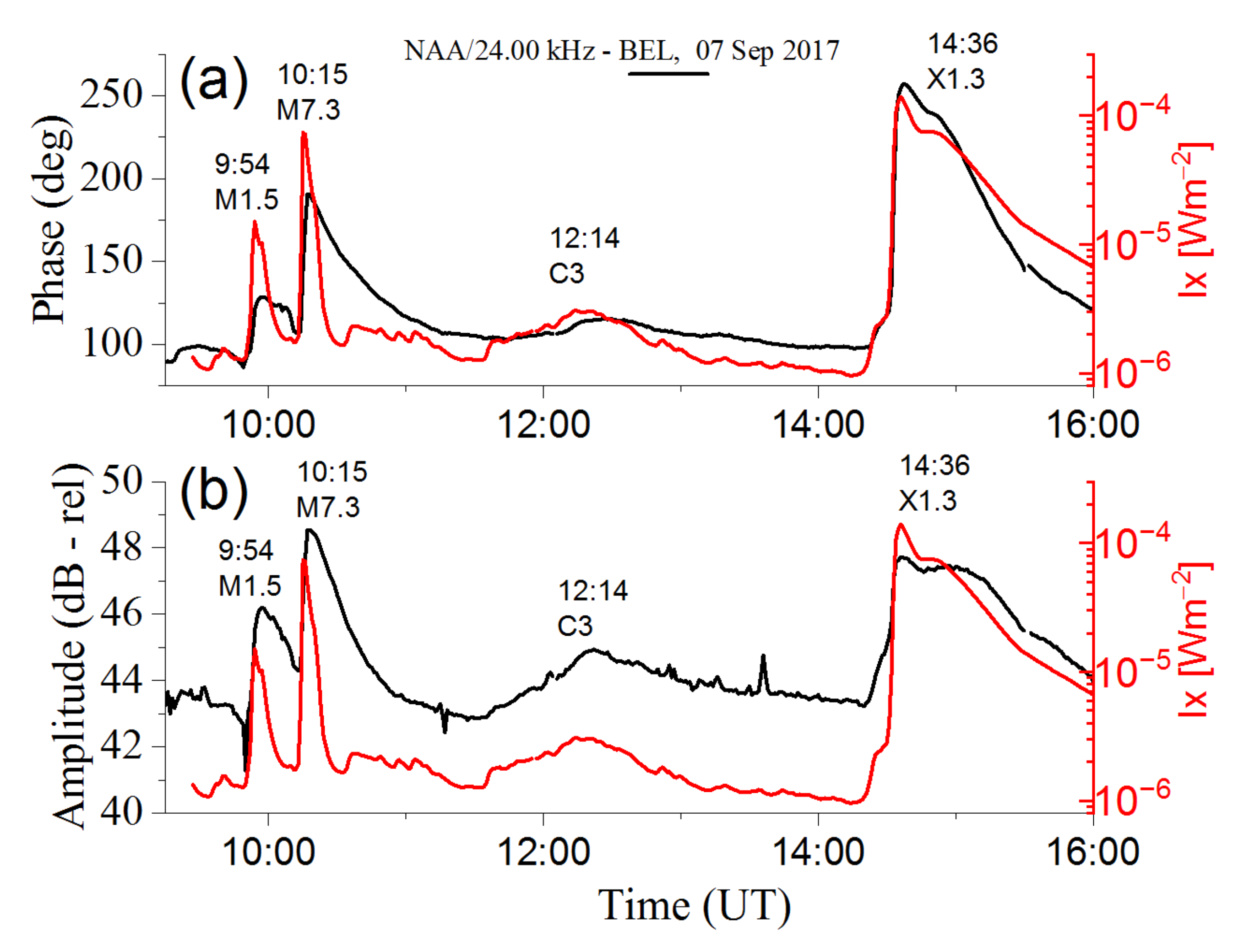
| X1.3 07.09.2017 | 14:20 | 14:36 | 14:55 | 4.50 | 159 | 1 | 1.39 × 10⁻⁴ | 2673 |
Publisher’s Note: MDPI stays neutral with regard to jurisdictional claims in published maps and institutional affiliations. |
© 2021 by the authors. Licensee MDPI, Basel, Switzerland. This article is an open access article distributed under the terms and conditions of the Creative Commons Attribution (CC BY) license (https://creativecommons.org/licenses/by/4.0/).
Share and Cite
Srećković, V.A.; Šulić, D.M.; Vujčić, V.; Mijić, Z.R.; Ignjatović, L.M. Novel Modelling Approach for Obtaining the Parameters of Low Ionosphere under Extreme Radiation in X-Spectral Range. Appl. Sci. 2021, 11, 11574. https://0-doi-org.brum.beds.ac.uk/10.3390/app112311574
Srećković VA, Šulić DM, Vujčić V, Mijić ZR, Ignjatović LM. Novel Modelling Approach for Obtaining the Parameters of Low Ionosphere under Extreme Radiation in X-Spectral Range. Applied Sciences. 2021; 11(23):11574. https://0-doi-org.brum.beds.ac.uk/10.3390/app112311574
Chicago/Turabian StyleSrećković, Vladimir A., Desanka M. Šulić, Veljko Vujčić, Zoran R. Mijić, and Ljubinko M. Ignjatović. 2021. "Novel Modelling Approach for Obtaining the Parameters of Low Ionosphere under Extreme Radiation in X-Spectral Range" Applied Sciences 11, no. 23: 11574. https://0-doi-org.brum.beds.ac.uk/10.3390/app112311574