
A Mobile Robot with Omnidirectional Tracks—Design and Experimental Research


Faculty of Mechanical Engineering, Wroclaw University of Science and Technology, Wybrzeże, Wyspiańskiego 27, 50-370 Wroclaw, Poland
*
Author to whom correspondence should be addressed.
Appl. Sci. 2021, 11(24), 11778; https://0-doi-org.brum.beds.ac.uk/10.3390/app112411778
Submission received: 18 November 2021
/
Revised: 5 December 2021
/
Accepted: 7 December 2021
/
Published: 11 December 2021
(This article belongs to the Special Issue Advances in Industrial Robotics and Intelligent Systems)
Abstract
:This article deals with the design and testing of mobile robots equipped with drive systems based on omnidirectional tracks. These are new mobile systems that combine the advantages of a typical track drive with the advantages of systems equipped with omnidirectional Mecanum wheels. The omnidirectional tracks allow the robot to move in any direction without having to change the orientation of its body. The mobile robot market (automated construction machinery, mobile handle robots, mobile platforms, etc.) constantly calls for improvements in the manoeuvrability of vehicles. Omnidirectional drive technology can meet such requirements. The main aim of the work is to create a mobile robot that is capable of omnidirectional movement over different terrains, and also to conduct an experimental study of the robot’s operation. The paper presents the construction and principles of operation of a small robot equipped with omnidirectional tracks. The robot’s construction and control system, and also a prototype made with FDM technology, are described. The trajectory parameters of the robot’s operation along the main and transverse axes were measured on a test stand equipped with a vision-based measurement system. The results of the experimental research became the basis for the development and experimental verification of a static method of correcting deviations in movement trajectory.
1. Introduction
In 2018, the world mobile robot market was worth USD 19 billion [1]. On the basis of the latest forecast, it is estimated that by 2023 its value will have nearly tripled. These robots have already moved from closed research centres and innovation fairs to the reality of everyday life. Autonomous transport vehicles used for supplies in storage facilities, autonomous mowers in house gardens, smart vacuum cleaners in homes, teleoperated robots, or bomb disposal robots are not only becoming a common element in company equipment, but also a commodity purchased by the average consumer [2,3]. Terrestrial mobile robots can be categorised using a number of criteria, and their constructed systems differ in terms of locomotion types. They can be wheeled, stepping, tracked, or ball balancing robots [4].
Wheeled robots are the most recognized, investigated and frequently used group of mobile robots. They achieve the highest speeds on flat surfaces. Their downside, however, is their poor ability to operate in difficult terrain, with some of them being vitiated by a significant turning radius [5]. Currently, research on improving their mobility in difficult terrain is being conducted. One new solution that has been proposed are hybrid wheeled–stepping robots [6,7,8].
At the opposite end of the robot spectrum are stepping robots, i.e., devices that are characterised by the best adaptation to overcome obstacles in terrain. Important disadvantages of their most common versions is low movement speed and complex problems related to the stepping control methodology (e.g., problems with maintaining balance during dynamic stepping in unknown terrain) [9]. In recent years, research on improving the movement speed of stepping robots has been conducted [10,11].
Tracked robots can be classified as a compromise between wheeled and stepping robots. Tracks allow for the mobility of the robot in difficult terrain, while also helping them to maintain a satisfactory movement speed. This type of locomotion has been recognised, investigated and used to a significantly higher degree than stepping systems [12].
Ball-balancing robots, also called ballbots, are robots in which the wheelset system is a ball [13]. This locomotion type, apart from ensuring holonomic control, is a successful solution in robot locomotion that is used to demonstrate technology, and in toys or presentation robots. It is visually attractive. The ballbot group also encompasses robots with a spherical outer casing, or a casing resembling a spherical shape [14,15]. Due to such a construction, these robots can not only achieve a high speed, but can also overcome water obstacles in difficult terrain.
Mobile robotics is now at the stage of dynamic development, where it quickly adapts to novel technological solutions while maintaining some previously used ones. Various simple solutions are successfully used in modern applications. Paper [16] addresses the issues of the hybridization of animals and machines, as well as the use of robots for research on animals. Many of their functions, such as the movement of a mechanical fish, are performed by simple mechanical systems. Paper [17] describes the construction of a mobile robot, in which the stepping movements of 4 legs are produced by a single drive.
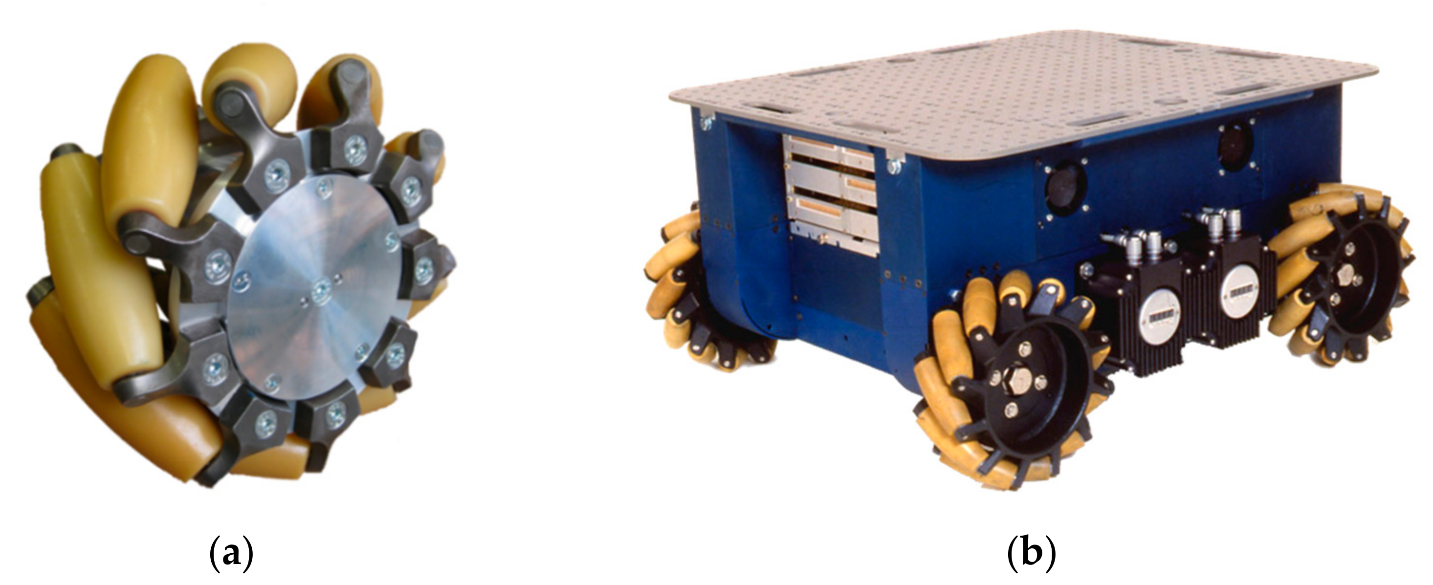
An example use of an existing and well-investigated solution can be seen in Mecanum wheel systems. They were patented in 1972 by Swedish engineer Bengt Erland Ilon [18]. The wheels, due to top free rotation rollers oriented at 45° on the wheel circumference, as well as appropriate steering, allow vehicles to move in any direction on a flat surface [19] (Figure 1). Another alternative is the use of transversal rollers oriented at 0°—although such a solution means that the implementation of an optimal wheel with a minimum gap may require an expensive manufacturing process [20].”
A four-wheeled robot with Mecanum wheels (Figure 1b), which is driven by four independent motors, can move in any direction on a plane without the necessity to rotate [19,23,24]. A robot equipped with Mecanum wheels is holonomic, so the number of controlled degrees of freedom is equal to the number of degrees of freedom that are held. This is of particular significance in the case of robots that operate in very limited spaces. Fork-lifts and transport robots with Mecanum wheels, which are therefore able to move in any direction, can be used in storage facilities and production halls in which there is a lot of equipment and a large number of storage racks in a small space.
Apart from the whole array of advantages, Mecanum wheels also have considerable disadvantages: robots and vehicles equipped with such wheels need flat, even and clean surfaces. However, there have been many investigations aimed at improving the locomotion of such systems in difficult terrain [25]. The vibration of rotating rollers, which occurs during motion, is another drawback of Mecanum wheels. The reason for this vibration is the cyclical shifting of the load between the subsequent rollers of a wheel [26]. In most applications, the vibration will not have a significant impact on the robot’s operation, however, in some specific uses it can have a significant influence on it [27]. Another potential issue is the distribution of load on the floor surface. Due to their structure, Mecanum wheels have a small wheel-surface contact area. To improve the force distribution and to prevent defects of the surface on which the robot moves, additional, surplus wheels are used in numerous applications for the purpose of reducing the impact of load on the surface. In some applications, non-driven castor wheel types are used, with additional driven Mecanum wheels being used in some others [28].
In recent years, research has been conducted on the possibility of combining Mecanum wheels with a classical drive track. Mobile robots with such a track system have all the advantages of vehicles with Mecanum wheels, but do not take on their disadvantages. They can move on uneven, dirt-covered terrain and can carry heavier loads due to the multiple number of rollers in the tracks. Systems with such a drive can be used as mobile storage robots, automated construction machines (excavators, drilling rigs) [29], inspection or rescue robots, transport platforms and bomb disposal robots. The use of multidirectional tracks in the construction of mobile robots significantly increases their maneuverability.
In 1999, in Isod’s work [30], the issue of multidirectional tracked robots was discussed. Such attempts to transfer the properties of Mecanum wheels to tracked wheels were made in 2015 and are described by Zhang [31].
In 2017, a German company, IVA Johann GmbH, in cooperation with scientists from the Bremer Institut für Produktion und Logistik, presented a commercial prototype of a mobile robot equipped with multidirectional tracks [29]. In 2018, the results of simulation research conducted by Zhang [32] on a platform equipped with multidirectional tracks were published. In 2020, Fang published research results involving the construction and tests of a fork-lift equipped with multidirectional tracks, which was designed to transport loads of a maximum of 2 tons [33]. During the research, which was both experimental and numerical, it was shown that a robot with multidirectional tracks preserves its holonomic characteristic.
The paper published by Huang discussed mobility in difficult terrain [34]. During movement along the robot’s main axis, multidirectional tracks preserve the robot’s ability to overcome terrain obstacles, such as embankments, stairs, thresholds or curbs. In the case of transverse movement to the robot’s main axis, the ability to overcome thresholds and steps was significantly reduced. Due to the ability to overcome obstacles while travelling along the main axis, the new robot will replace systems with Mecanum wheels in warehouse facilities and production halls that may have floors with uneven surfaces, thresholds and kerbs.
Simulation research results on rectilinear motion in the transverse direction of a robot with multidirectional tracks are presented in [33]. It was demonstrated that the robot’s motion trajectory becomes curved during such motion, which was also confirmed by the experimental research discussed in [32]. Deviations from the rectilinear path depend on the robot’s mass, and such deviations increase with a decrease in system mass. An article written by Huang [34] also discusses research on the transverse motion of a robot on a smooth and slippery surface and includes the problems resulting therefrom.
Primarily robots with longitudinally symmetric non-overlapping tracks were investigated in the publications referred to above, and only in one case were robots with symmetric and partly overlapping tracks scrutinized. However, the publications do not discuss issues related to the applications of non-symmetric tracks, nor do they discuss other track systems. Research on the influence of load on driving properties has been conducted for robots with a mass of a maximum of 5 tons. The issue of vibration during the locomotion of robots with multidirectional tracks was not discussed. No attempt to compensate for deviations of direction during locomotion was made.
In this paper is developed a new mobile robot with a drive system that uses multidirectional tracks. The research encompasses the ability of a prototype to perform basic manoeuvres, i.e., motion along the main and transverse robot axes. A static method of improving motion parameters by correcting control parameters was developed and verified. The tests were conducted on a prototype made with fused deposition modelling (FDM) 3D printing technology on a test bench equipped with a vision-based measurement system.
2. Materials and Methods
2.1. Construction of a Mobile Robot with Multidirectional Tracks
A classical vehicle with a track drive system (excavator, bulldozer, tank, armoured personnel carrier, bomb disposal robot, etc.) is made of a body and two continuous track systems located symmetrically to the body (Figure 2a). A vehicle with a drive system with multidirectional tracks is equipped with four continuous track systems, which can usually be positioned in various ways with regards to the vehicle’s body. The typical schemes of continuous track positions encompass tracks that are completely overlapping (Figure 2b), tracks that are partially overlapping (Figure 2c), as well as systems with non-overlapping tracks (Figure 2d).
It was assumed that the mobile robot to be constructed would have the structure of a symmetrical system with completely overlapping tracks, i.e., it will be made of a body and four parallel track drive systems of equal length with completely overlapping tracks (Figure 2b).
During contact between the continuous track and the surface, tractive force is generated. This force is necessary for a vehicle to move. A large surface-track contact area and an appropriately adjusted track preload result in a lower unit pressure of the track when compared to the wheel. A standard, single continuous track system is made of a track located between the drive wheels, idler, road wheels and return rollers (Figure 3a). In some track vehicles (e.g., excavators), there are solutions in which the drive wheels and idlers also take the load-carrying capacity (Figure 3b). This type of powertrain was also selected for the designed mobile robot. However, due to the large radius of the drive wheels and idlers in relation to their spacing, no extra road wheels were used (Figure 3c).
Tracks in the continuous track system are composed of a closed sequence of several dozen links that are connected to one another with rotating pairs. In the case of multidirectional tracks, each link is equipped with an additional rotating roller positioned at angle γ (usually 30° < γ < 60°) to the link axis. The view of a single link with length a, width b, and height h, and also a cylindrical roller with radius rr,, is presented in Figure 4.
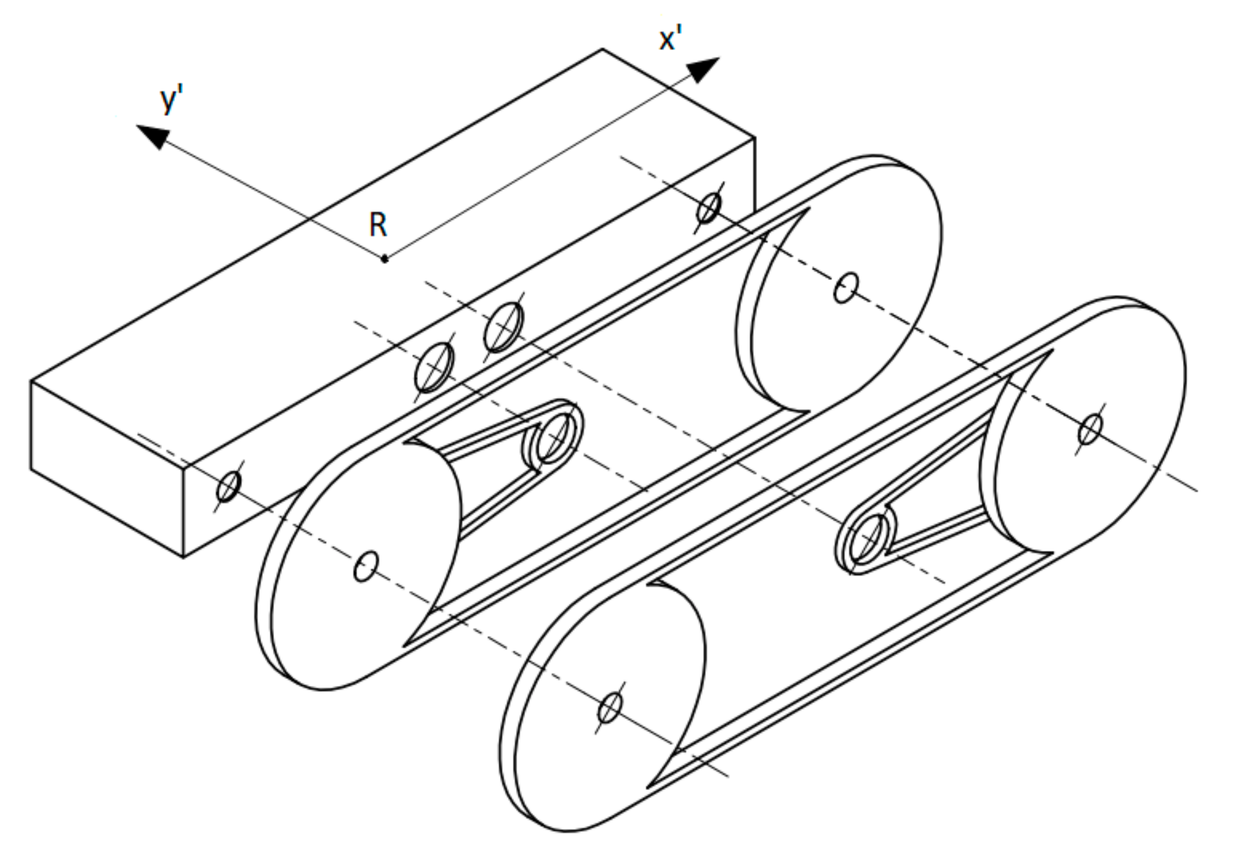
The designed mobile robot is equipped with four independent continuous track systems with multidirectional tracks that have only drive wheels and idlers. It is a four-degrees-of-freedom system. The drive is transferred from the rotating drives to the drive wheels using belts. In the middle part of the robot’s body, at point R, the local x’y’ coordinate system is located. The kinematic scheme of the robot is shown in Figure 5.
It was assumed that the designed robot would be used indoors (residential buildings, offices, warehouse facilities, production halls, etc.). Therefore, its dimensions must be adapted to overcome the typical obstacles seen in such places: doors, thresholds, staircases, etc. The robot should move at a maximum speed of vR = 0.2 m/s, which is the speed considered acceptable for a robot moving in a ‘human environment’ [35]. This means that the maximum track speeds 1, 2, 3, 4:
The resulting basic dimensions are described in Table 1.
Figure 6 shows an overview of the developed solid model of the robot and the detailed views of the solid model of the track system.
Figure 7 shows the views of a single continuous multidirectional track with its own drive system. The continuous track system is composed of a track, an idler and a drive wheel. In each track segment there is one cylindrical rotating roller. The drives are located in the central part of the robot. The active moment is shifted to the drive wheel using transmission with a toothed belt.
The track drive systems, track links, rollers and the body of the robot were made using incremental FDM technology. The material used is PET-G, which is a polymer characterised by low shrinkage and high mechanical resistance. The free rollers rotate on steel axes. There are plastic slip rings between the rollers and the mount, which is connected to the track plate. The rollers consist of a printed core, onto which the tyres are pulled. The tyres of the rollers, also made using FDM technology, are made of thermoplastic polyurethane with a Shore scale hardness of 40D. The view of the finished prototype of the mobile robot is presented in Figure 8.
The motor is connected to the drive wheel by a reduction pulley transmission system with a reduction ratio of ik = rs/rks = 0.25. For the assumed maximum robot motion speed vr (Table 1), the maximum angular velocity of the motor ωs was determined from the following equation:
The rated active moment of motor Ms was selected using the simplified method of the experimental measurements of the robot’s motion resistance in the longitudinal and transverse direction using a tensometric force sensor. The highest motion resistance was measured experimentally during motion in the direction perpendicular to the main axis, and is expressed as the maximum force that excites motion in a set direction, which was 13 N. It was assumed that the motor moment Ms should be greater than:
On the basis of the calculations made to design the prototype construction, POLOLU-2274 motors were selected with a torque of Ms = 0.57 Nm, and a nominal speed of = 21.99 rad/s. Each motor is equipped with a magnetic encoder that provides 48 counts per revolution, and therefore one complete revolution of the wheel will provide 2249 pulses, with a drive wheel accuracy of Δϕs = 0.0007 rad.
2.2. Control System of the Mobile Robot with Multidirectional Tracks
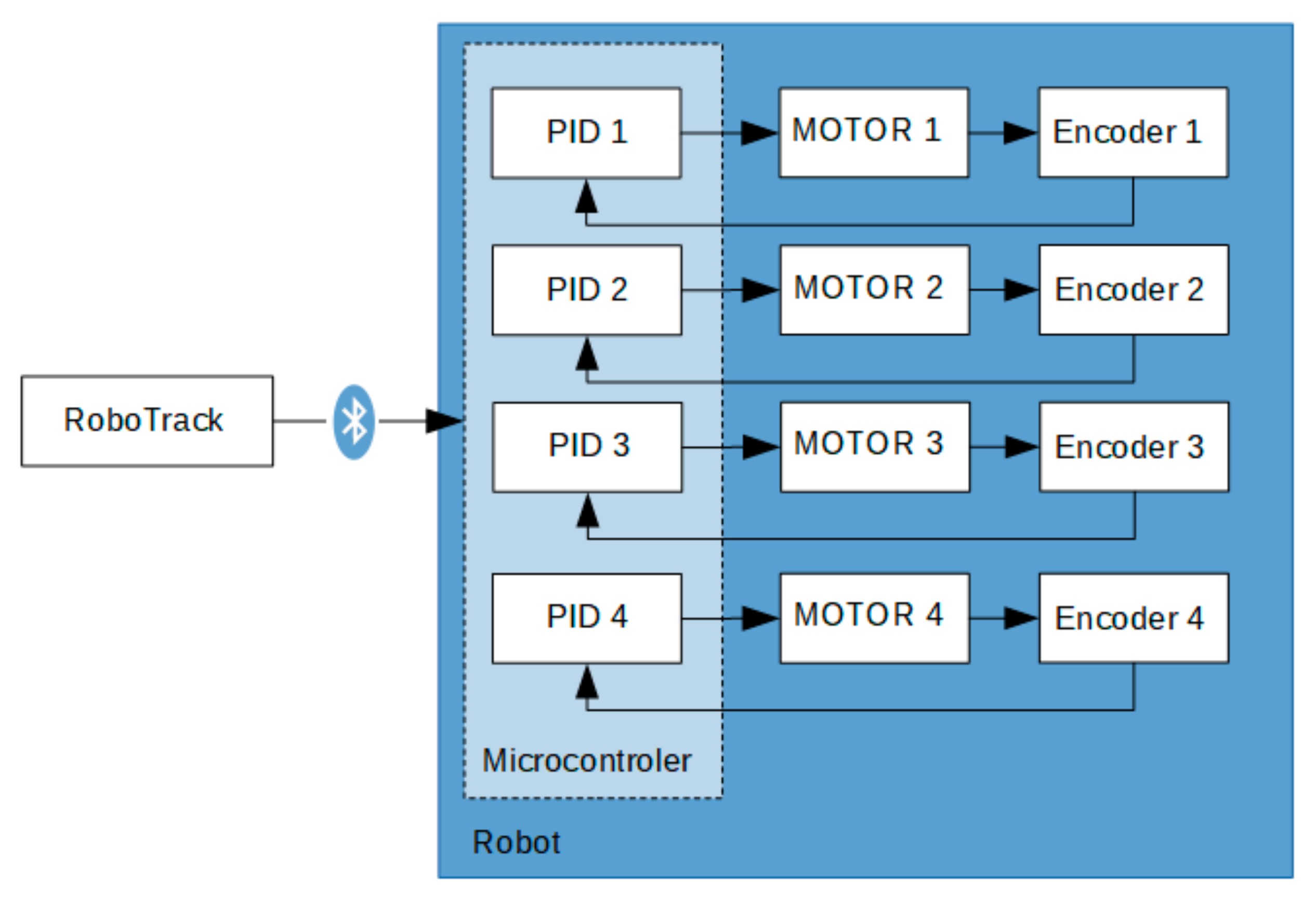
For the purpose of exciting the set robot motion, it is necessary to have an appropriately designed system and control algorithms. The mobile robot has four drives that independently excite the motion of each track (Figure 5 and Figure 8). Thus, a control system is required to control the robot. The control system should have four control regulators of speed ωsi of motor i (i = 1, 2, 3, 4), which start the drive wheels of the continuous tracks. In the robot prototype, the speed control of the used DC motors will have the form of a pulse width modulation (PWM) signal. The general scheme of the developed robot’s control system is presented in Figure 9.
Motor i, which excites the motion of the continuous track system i, is individually controlled using a PIDi regulator operating in the feedback loop with a frequency of 50 Hz. The value of vR(t) is the set speed of the entire robot, the value of ωTi(t) is the value of the set speed of track motor i (i = 1, 2, 3, 4), Ei(t) is the control error, Ui(t) is the steering signal, Pi(t) is the PWM value responsible for motor control DC, ωMi(t) is the actual motor rotational speed, Θi(t) is the motor rotation angle measured with an encoder, while ωi(t) is the motor angular speed. The scheme of the speed regulator of continuous track system i is presented in Figure 10.
A RoboTrack control program was developed to control the movement of the robot. The program is run on an external PC.
The programme is responsible for planning the robot’s motion trajectory and for sending the set speed values ωTi(t) for particular motors i to the robot’s control system based on speed values set by the user. RoboTrack also ensures the on-line registration of ride parameters. Communication between the external PC and the mobile robot is performed with a Bluetooth communication link
The excitation of the robot’s motion along the set trajectory requires a suitable control of speeds v1, v2, v3, v4 of tracks 1, 2, 3, 4. This paper discusses robot motion along two trajectories: a straight line μw at constant speed vRx along the longitudinal axis, and a straight line μp at constant speed vRy along the robot’s transverse axis (Figure 11). In the case of motion along the longitudinal axis at speed vRx, the tracks should move at the same speeds (Figure 11):
while during motion along the transverse axis at speed vrx, the tracks’ speed takes the following values:
2.3. External Measurement Test Bench
The mechanical prototype proposed in this paper is not able to develop self-localization [36]. The localization of the mobile robot is determined with an external measurement test bench, the general scheme and view of which are presented in Figure 12. The vision-based measurement system was made of a camera located perpendicularly to the measured area. The ELP-USBFHD04H-MFV camera with a resolution of 1920 × 1080 px was located at the height h = 1.95 m with regard to the main coordinate system xy (Figure 12).
The measuring accuracy of the bench was checked using a printed calibration sheet with ArUco markers (Figure 13). The position reading error δl of the marker was less than 0.008 m and the orientation angle error δα was no more than 0.5°.
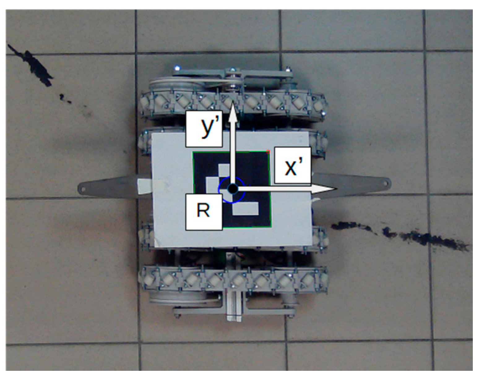
The vision-based system records and analyses images with a frequency of 25 Hz (frames/s). In order to allow for the detection of the robot’s position in a camera image, the vision marker ArUco was placed on its top surface (Figure 14). The ArUco marker is a print on a flat tile with white and black rectangles. Owing to the precisely defined distribution of these areas, the marker can transfer its ID number, and it is therefore possible to recognize its presence in a ready image, as well as to determine its linear and angular position. For known dimensions, it is also possible to conduct a programmable estimation of its location in three-dimensional space. The middle of the marker is located in point R on the robot’s body (Figure 14). During the measurement, the whole marker must be located in the camera vision area—this efficiently reduces the observation area to the area of the following dimensions: a = 0.75 m, b = 1.30 m.
The robot is controlled by RoboTrack software (Figure 15), which allows robot motion to be controlled and track and motor motion to be registered. The software was integrated with a VisionM module that allows the covered distance to be measured and recorded. This module is based on OpenCV libraries that are extended with OpenCV Contrib [37] modules. Its task is the online analysis of individual image frames recorded by a camera placed on the test stand. The module provides data on the angular orientation of the tracked robot, its current location and the distance covered, which are recorded in real time.
2.4. Static Correction Method of the Robot’s Locomotion Direction
During the motion of the mobile robot with the continuous track system with multidirectional tracks travelling at a constant speed, the phenomenon of curved trajectories may take place [24,27]—the middle R of the robot’s body deviates from the trajectory, and the orientation angle αR of the body changes. The deviations from the straight-line trajectory depend on the robot’s mass, and they increase with the system’s mass [27]. During movement along the transverse axis, the problems with maintaining straight line movement become even more significant when the robot moves on a slippery surface. This disadvantageous phenomenon can be prevented by the introduction of suitable corrections to the set speeds of particular continuous tracks.
For the purpose of maintaining the robot’s motion along the set straight line trajectory, the fixed orientation angle αR of the robot’s body should be ensured by introducing suitable corrections of track speeds.
A difference in the orientation αR of the body, i.e., between the real and set robot position, results from the robot’s body rotation at constant angular speed ωr. The rotation can be reduced by forcing the body to rotate in the opposite direction by making appropriate changes in track set speeds.
A simplified model of the change in the robot’s body orientation and motion direction (Figure 16) was proposed, which entails the introduction of virtual tracks located between tracks 1 and 2,—marked as L12, with 3 and 4 being marked as R34. The speed vk of the virtual tracks excites the corrective rotation of the body, which eliminates the change of orientation, can be determined from Equations (6) and (7). These equations take into consideration the change in the angle ΔαΡ of the orientation at time Δt, structural dimension c describing the distance between the pairs of continuous tracks, and an empirical adjustment factor cf resulting from the surface type and the adhesion of the rotating rollers:
In the case of the robot’s motion along the longitudinal axis, the correction of track speed involves its suitable increasing or decreasing by value vk according to the following formula (Figure 17a):
Speed correction vk for motion along the robot’s transverse axis consists of differentiating the speed on each pair of tracks according to formula (Figure 17b):
2.5. Experiment Plan
A number of experimental tests of the mobile robot were carried out on the test stand in order to verify the operation of the proposed drive systems and to determine the basic kinematic properties of the movement.
The tests encompassed a number of rides on straight line trajectory μz located along the longitudinal and transverse axes of the robot. Various measurements of the location, the linear and angular speeds of the robot’s body, the rotation angle and angular speeds of the drive wheels, and also the speed of the tracks were conducted during the rides. The research was conducted on a specially designed test bench equipped with a vision-based location measurement system. Figure 18 presents the scheme of the experiment carried out on the measurement test bench.
Ride tests were conducted at two stages. In the first part of the experiment, the set values of the linear speeds of all the tracks did not take into account the correction parameters. In the second part of the experiment, the speeds of particular drives were differentiated by the correction value, which was calculated on the basis of the proposed model of ride trajectory correction.
3. Results
The results of the measurements obtained during the investigated robot rides along the longitudinal and transverse robot axes are presented and discussed below. The tests and measurements were carried out on the designed measurement test bench (Figure 12). The length of the tested trajectory was limited by the area of the test bench. The trajectory waveforms μR (xR, yR), the dependence of change Δα οn time, and the change of the coordinates xR, yR over time were plotted on the basis of the stationary measuring system, while the speeds of the individual tracks were determined on the basis of the angles indicated by the encoders in relation to time.
3.1. Robot Ride Tests
The tests of the robot’s rides along the longitudinal axis were conducted in accordance with the scheme shown in Figure 18a. The robot moved along the planned straight-line trajectory μt by length L1 = 1.2 m at the constant speed vRx = 0.12 m/s.
The scheme presented in Figure 18b shows the plan of the research on the robot’s rides along the transverse axis. The robot moved along the planned straight-line trajectory μt by length L2 = 1.2 m at constant speed vRy = 0.12 m/s.
During the research, the waveforms of real ride trajectories μR (xR, yR), the changes of body orientation angle Δα, coordinates xR, yR of point R on the robot’s body, and the real linear speeds v1, v2, v3, v4 of the tracks calculated on the basis of encoder indications were measured and registered. Figure 19, Figure 20, Figure 21 and Figure 22 show the measurement results for rides along the longitudinal axis, while Figure 23, Figure 24, Figure 25 and Figure 26 depict the measurement results of the robot’s rides along the transverse axis.
The experiment showed that during the rides the real, linear speeds of tracks vi adopted the values of the set speeds, vRx and vRy. In the case of longitudinal motion, the largest speed errors occurred at the start-up of the robot’s motion. After the stabilisation of speed, the errors took significantly smaller values (Figure 22). In the case of transverse motion, the values of the track speed errors occurring at the start-up were comparable to the deviations observed during the whole ride (Figure 26). It should, therefore, be noted that no such error jump between the set and real speed in transverse motion was observed. Despite the speed jump at start-up, the maximum deviation between the real and set speed Δvi was Δvi =0.02 m/s for the longitudinal motion, and Δvi =0.03 m/s for the transverse motion (Figure 22 and Figure 26).
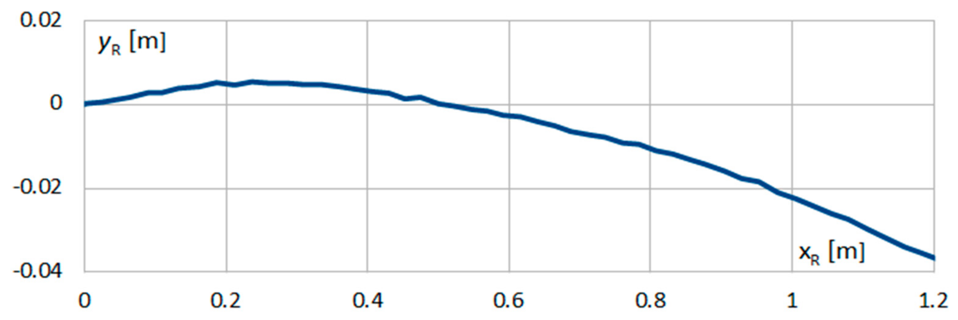
In both longitudinal and transverse motion, deviations from the planned trajectory were observed in the form of a curved ride and a change in the orientation of the robot’s body (Figure 20 and Figure 24). The location error of point R was determined to be ΔyR = yRT – yR. In both the longitudinal and transverse motion, the set trajectory is a straight line overlapping with the X axis of the measurement test bench coordinate system. Due to this, for both rides the theoretical location of point R in relation to the Y axis is yRT = 0. Location deviation ΔyR = yR.
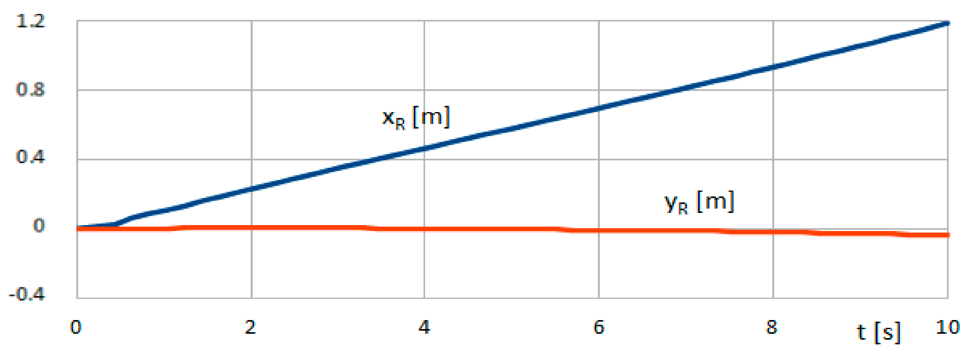
In the case of the longitudinal motion, the final location error of point R was ΔyR= 0.037 m (Figure 21), while the orientation change was Δα =5° (Figure 20) at time t = 10 s.
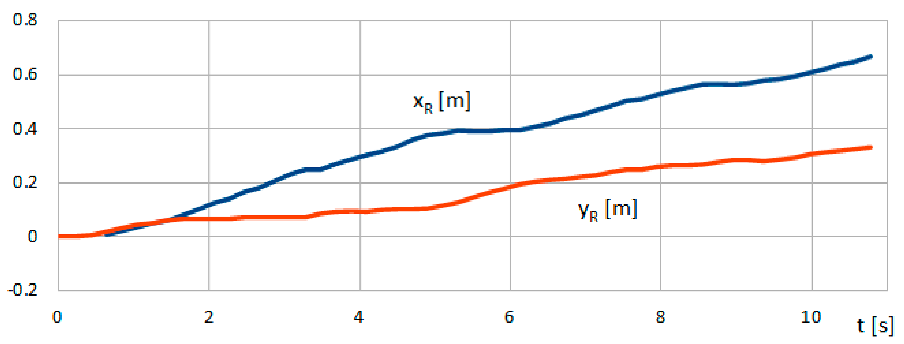
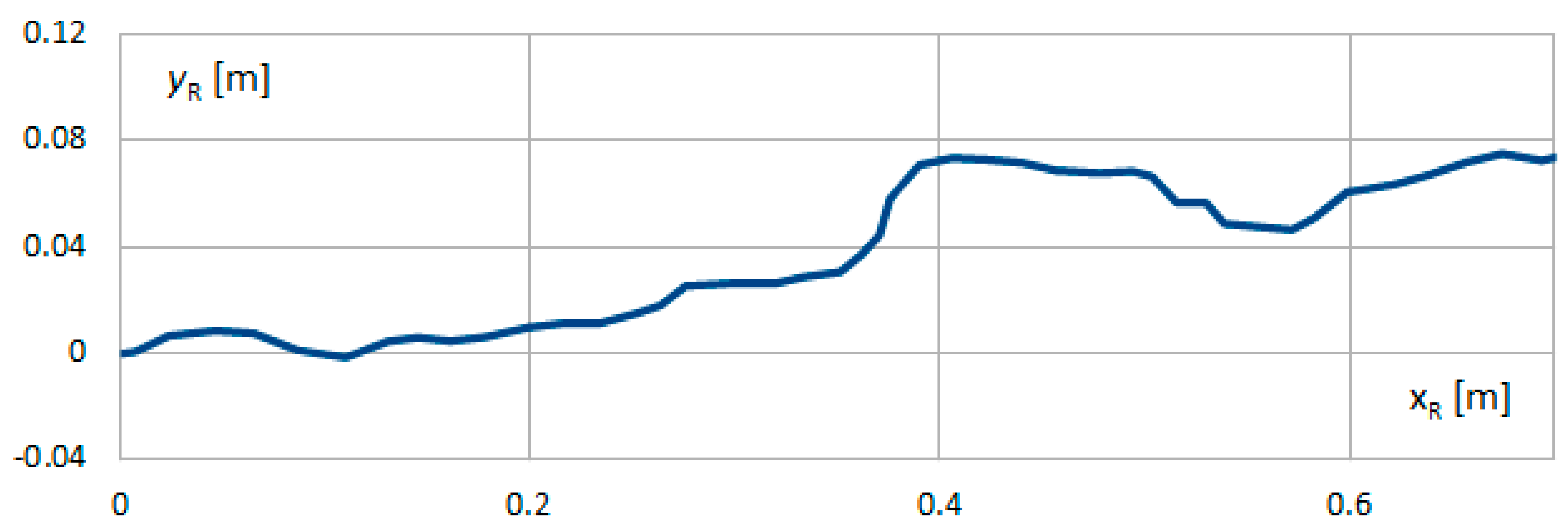
During the transverse motion, the robot did not cover the whole planned distance (L2 = 1.2 m), and the measurement was interrupted after it had covered the distance of 0.7 m (Figure 25) because the robot overstepped the measurement area boundary in the direction of the y axis. In the case of the transverse motion, the final orientation change was Δα = 35° (Figure 24), and the location error of point R was ΔyR= 0.36 m (Figure 25) at time t = 10.8 s.
The analysis of the waveforms of changes in the orientation angle Δα of the robot’s body at time t indicated that they had a linear nature. This was confirmed by the conducted statistical analyses. The value of the Pearson linear correlation starts to be higher at 0.97 onwards for both the longitudinal and transverse motions.
3.2. Tests of Robot Rides with Consideration for the Static Correction Method of Ride Direction
The phenomenon of the change in the angle Δα of body orientation had a linear nature, and therefore the application of the static correction method set out in Section 2.5 was justified. On the basis of the planned changes of orientation angle Δα during a ride (Figure 20 and Figure 24), the values of speed vkw, corrections for the longitudinal motion, and vkw for the transverse motion, were calculated using Formulas (6) and (7).
In the calculations, the adaptation factor cf was taken into account. For the given robot’s dimensions, the value of the c parameter was 0.16 m. With consideration for the type of substrate (track link rollers made of TPU filament with a hardness of 40D moving on ceramic tiles), the value of the factor was determined, empirically, to be cf = 4.4.
The corrective speed values, obtained using Formula (7), were vkw = 0.04 m/s for the longitudinal motion and vkp = 0.35 m/s for the transverse motion. The corrective speed value vkp = 0.35 m/s were restricted to 0.2 m/s due to the limitations of the drive and control systems of the used equipment.
For the obtained values of the corrective speed, two more tests of the robot’s rides along the longitudinal and transverse axes were conducted. Figure 27, Figure 28, Figure 29 and Figure 30 present the results of the measurements for the rides along the longitudinal axis, while Figure 31, Figure 32, Figure 33 and Figure 34 show the results for the measurements of the robot’s rides along the transverse axis.
The measurements showed that the obtained linear speeds of the tracks vi assume values close to the set speeds vRx and vRy, which were corrected by values vkw and vkp. The differences between real value vi and set value vRx for the longitudinal motion were Δvi < 0.02 m/s (Figure 30), disregarding the temporary error jump at the start-up. For the transverse motion, the same value was Δvi < 0.04 m/s (Figure 34). In this case, analogically as in the transverse motion without correction, no temporary error jump of speed at start-up was recorded. Therefore, the worsening ability to maintain the set speed vi of the tracks in the transverse motion was observed, which was probably caused by the occurrence of low friction between the surface and the track.
Both in the case of the transverse and longitudinal motion, there was a significant flattening of the trajectory curve (Figure 27 and Figure 31). In the presented case, the final change of orientation angle Δα of the body during longitudinal movement after the introduction of corrective speeds vkw was 1.4° (Figure 28), while the final point R location error was ΔyR= 0.01 m (Figure 29). A fourfold improvement of the drive parameter Δα was obtained (Table 2).
In the case of transverse motion without speed correction, the robot did not cover the whole planned distance (Figure 25). Moreover, the measurement was stopped after covering 0.7 m at time t = 9 s (Figure 33), because the robot crossed the boundary of the measuring field in the direction of the Y axis. The same part of the trajectory was taken into account when analysing lateral movement while both considering and not considering, the correction of the driving (Figure 33).
The change of body orientation Δα after t = 9 s, i.e., at the time equal to the longitudinal drive without speed correction was 11° (Figure 32), while the location error was ΔyR = 0.07 m (Figure 33).
In the transverse motion, the observed improvement trajectory curve was smaller than in the case for longitudinal motion. This resulted from, among other things, a 50% decrease in the required corrective speed vkp, which took place for equipment-related reasons. The so-reduced correction is not perfectly efficient and therefore it did not allow for the complete improvement of the robot’s trajectory. The obtained improvement (over a threefold reduction of error Δα (Table 2)), however, proved the correctness of the used method in the transverse motion of the robot.
The obtained measurement results of drive parameters were statistically analysed and are presented in Table 2.
4. Discussion
The paper presents a solution for a robot equipped with completely overlapping multidirectional tracks with a symmetrical roller position. A light robot prototype was designed and constructed using additive manufacturing technology to be later used in experimental research on a specially constructed test measurement bench. The robot’s parameters were examined along the longitudinal and transverse axes.
The experimental research without ride direction correction confirmed the occurrence of the effect of motion trajectory deviation during transverse motion. Similar effects of the trajectory curve were observed during the simulation tests of the robot with non-overlapping tracks [27] and with partly overlapping tracks [24].
The data quoted in the references indicate a 3.8% deviation between the theoretical speed and the one obtained in the dynamic simulation during transverse motion, and less than a 1% deviation in the main motion. In these references, no quantitative data was presented regarding the change in the angular orientation of the robot.
The data obtained during the conducted experiment showed a deviation increment of 0.016 rad/s in the longitudinal motion, and 0.133 rad/s in the transverse motion.
Such significant values of the trajectory curve probably result from the mechanical imperfections of the prototype, which were probably due to the adopted drive system’s structure without idling rolls and the used manufacturing technology. The fact that the track links and rollers were made of TPU filament, were of 40D hardness in the Shor scale, and had a low friction coefficient resulted in low adhesion of the robot to the surface. It was shown that this effect could be corrected using a suitable control system. The proposed static method of ride direction correction performed this role. The application of the continuous track speed correction allowed the angular deviation during longitudinal motion to be reduced to 0.007 rad/s, and to 0.019 rad/s during transverse motion. Despite the used correction by a value smaller than would result from the transverse motion calculations, a significant improvement in trajectory parameters was observed. This confirms the correctness of the used method and creates opportunities for further research and experiments.
The downside of the used correction method is the fact that it is a static method, which means that it requires earlier experimental tests of a robot on a particular type of surface, with the results needing to be used as the basis for the determination of efficient correction parameters. The application of a dynamic method of ride direction correction would improve the performance even more, and, in effect, eliminate the consequences of deviations in trajectory during robot motion. In further research stages, the prototype will be equipped with additional body orientation angle measurement sensors, which will allow the use of dynamic motion direction correction.
5. Conclusions
The key considerations of this paper were the design and testing of a mobile robot with an omnidirectional track. The research confirmed the ability of the robot to drive omnidirectionally while maintaining a fixed body orientation. The use of multidirectional tracks in the construction of mobile robots significantly increases their manoeuvrability.
The obtained results clearly show that vehicles equipped with continuous track systems with multidirectional tracks can still be improved. The application of the approach, involving the compensation of mechanical imperfections with the use of additional sensors and appropriate control, will allow for an even more precise maintenance of the set motion direction. The mechanical design of the track system also had a great influence on the accuracy of the robot’s movement. Introducing additional road wheels and idlers or changing the material and geometry of the rollers in the track links will improve the contact between the track and the ground.
The development of systems equipped with continuous track systems could be used, inter alia, in the construction of equipment operating on narrow construction sites with numerous obstacles. Tracked machines, which are able to move in the transverse direction, would facilitate manoeuvring and contribute to reducing the number of accidents. Another potential area of application is the transport of small, yet heavy loads, in very limited spaces—in this case a uniform load distribution on the whole track could be of key significance for the usability of such vehicles.
Author Contributions
Conceptualization, M.F. and J.B.; methodology, M.F. and J.B.; software, M.F.; validation, M.F. and J.B.; formal analysis, M.F. and J.B.; investigation, M.F. and J.B.; resources, M.F.; data curation, M.F. and J.B.; writing—original draft preparation, M.F.; writing—review and editing, M.F. and J.B.; visualization, M.F.; supervision, J.B.; project administration, M.F. and J.B.; funding acquisition, J.B. All authors have read and agreed to the published version of the manuscript.
Funding
This work was supported by Grants-in-Aid at Wroclaw University of Science and Technology, Faculty of Mechanical Engineering, Poland, (No. 8211104160).
Institutional Review Board Statement
Not applicable.
Informed Consent Statement
Not applicable.
Data Availability Statement
Contact via email.
Conflicts of Interest
The authors declare no conflict of interest.
References
- Mobile Robots Market by Operating Environment (Aerial, Ground, and Marine), Component (Control System, Sensors), Type (Professional and Personal & Domestic Robots), Application (Domestic, Military, Logistics, Field), and Geography—Global Forecast 2023. Markets and Markets SE 3610. Available online: https://www.marketsandmarkets.com/Market-Reports/mobile-robots-market-43703276.html?gclid=CjwKCAiAksyNBhAPEiwAlDBeLNKlJXjxNs2XgzEZLhSGhCanirlhMDnTZn9YKn3O3mNjX-upD3xwBhoCD6wQAvD_BwE (accessed on 11 December 2021).
- Irobot. Available online: https://irobot.pl/pl/outlet/312-irobot-roomba-980-5060359281043.html (accessed on 27 October 2020).
- Husqvarna. Available online: https://www.husqvarna.com/pl/produkty/kosiarki-automatyczne (accessed on 27 October 2020).
- Moreno, J.; Clotet, E.; Lupiañez, R.; Tresanchez, M.; Martínez, D.; Pallejà, T.; Casanovas, J.; Palacín, J. Design, Implementation and Validation of the Three-Wheel Holonomic Motion System of the Assistant Personal Robot (APR). Sensors 2016, 16, 1658. [Google Scholar] [CrossRef] [Green Version]
- Wong, J.Y.; Huang, W. “Wheels vs. tracks”—A fundamental evaluation from the traction perspective. J. Terramech. 2006, 43, 27–42. [Google Scholar] [CrossRef]
- Bałchanowski, J. Modelling and simulation studies on the mobile robot with self-leveling chassis. J. Theor. Appl. Mech. 2016, 54, 149–161. [Google Scholar] [CrossRef] [Green Version]
- Sperzyński, P.; Bałchanowski, J.; Gronowicz, A. Simulation of motion of a mobile robot on uneven terrain. J. Theor. Appl. Mech. 2020, 58, 541–552. [Google Scholar] [CrossRef]
- Gronowicz, A.; Szrek, J. Design of LegVan Wheel-Legged Robot’sMechanical and Control System. SYROM 2009, 145–158. [Google Scholar]
- Machado, J.A.T.; Silva, M.F. An Overview of Legged Robots. In Proceedings of the MME 2006—International Symposium on Mathematical Methods in Engineering, Ankara, Turkey, 27–29 April 2006. [Google Scholar]
- Raibert, M.; Blankespoor, K.; Nelson, G.; Playter, R. BigDog, the Rough-Terrain Quadruped Robot. IFAC Proc. Vol. 2008, 41, 10822–10825. [Google Scholar] [CrossRef] [Green Version]
- Bledt, G.; Powell, M.J.; Katz, B.; Di Carlo, J.; Wensing, P.M.; Kim, S. MIT Cheetah 3: Design and Control of a Robust, Dynamic Quadruped Robot. In Proceedings of the 2018 IEEE/RSJ International Conference on Intelligent Robots and Systems (IROS), Madrid, Spain, 1–5 October 2018; pp. 2245–2252. [Google Scholar]
- Hornback, P. The Wheel Versus Track Dilemma. ARMOR 1998, 26, 33–34. [Google Scholar]
- Hertig, L.; Schindler, D.; Bloesch, M.; Remy, C.D.; Siegwart, R. Unified state estimation for a ballbot. In Proceedings of the Robotics and Automation (ICRA), 2013 IEEE International Conference on Robotics and Automation, Karlsruhe, Germany, 6–10 May 2013. [Google Scholar]
- Seeman, M.; Broxvall, M.; Saffiotti, A.; Wide, P. An Autonomous Spherical Robot for Security Tasks. In Proceedings of the Computational Intelligence for Homeland Security and Personal Safety, Alexandria, VA, USA, 16–17 October 2006. [Google Scholar]
- Guardbot. Available online: https://guardbot.org/ (accessed on 27 October 2020).
- Lee, Y.; Yoon, D.; Oh, J.; Kim, H.S.; Seo, T. Novel Angled Spoke-Based Mobile Robot Design for Agile Locomotion with Obstacle-Overcoming Capability. IEEE/ASME Trans. Mechatron. 2020, 25, 1980–1989. [Google Scholar] [CrossRef]
- Romano, D.; Donati, E.; Benelli, G.; Stefanini, C. A review on animal–robot interaction: From bio-hybrid organisms to mixed societies. Biol. Cybern. 2019, 113, 201–225. [Google Scholar] [CrossRef] [PubMed]
- Ilon, B.E. Wheels for a Course Stable Selfpropelling Vehicle Movable in Any Desired Direction on the Ground or Some Other Base. U.S. Patent US3876255A, 8 April 1975. [Google Scholar]
- Li, Y.; Ge, S.; Dai, S.; Zhao, L.; Yan, X.; Zheng, Y.; Shi, Y. Kinematic Modeling of a Combined System of Multiple Mecanum-Wheeled Robots with Velocity Compensation. Sensors 2019, 20, 75. [Google Scholar] [CrossRef] [PubMed] [Green Version]
- Palacín, J.; Martínez, D.; Rubies, E.; Clotet, E. Suboptimal Omnidirectional Wheel Design and Implementation. Sensors 2021, 21, 865. [Google Scholar] [CrossRef]
- Imetron GmbH. Mecanum Wheel. Attribution-ShareAlike 3.0 Unported (CC BY-SA 3.0). Available online: https://de.wikipedia.org/wiki/Mecanum-Rad#/media/Datei:Meacnum-Rad.png (accessed on 27 October 2020).
- Gwpcmu. Mecanum Wheel. Attribution 3.0 Unported (CC BY 3.0). Available online: https://en.wikipedia.org/wiki/Mecanum_wheel#/media/File:UranusOmniDirectionalRobotPodnar.png (accessed on 27 October 2020).
- Wu, M.; Dai, S.-L.; Yang, C. Mixed Reality Enhanced User Interactive Path Planning for Omnidirectional Mobile Robot. Appl. Sci. 2020, 10, 1135. [Google Scholar] [CrossRef] [Green Version]
- Palacin, J.; Rubies, E.; Clotet, E.; Martinez, D. Trajectory of a human-sized mobile robot using three omnidirectional wheels: From simulation to implementation. In press. Sensors 2021, 21, 7216. [Google Scholar]
- Yamada, N.; Komura, H.; Endo, G.; Nabae, H.; Suzumor, K. Spiral Mecanum Wheel Achieving Omnidirectional Locomotion in Step-Climbing. In Proceedings of the 2017 IEEE International Conference on Advanced Intelligent Mechatronics (AIM), Munich, Germany, 3–7 July 2017; pp. 1285–1290. [Google Scholar]
- Bae, J.-J.; Kang, N. Design Optimization of a Mecanum Wheel to Reduce Vertical Vibrations by the Consideration of Equivalent Stiffness. Shock. Vib. 2016, 2016, 5892784. [Google Scholar] [CrossRef]
- Moreno, J.; Clotet, E.; Tresanchez, M.; Martínez, D.; Casanovas, J.; Palacín, J. Measurement of Vibrations in Two Tower-Typed Assistant Personal Robot Implementations with and without a Passive Suspension System. Sensors 2017, 17, 1122. [Google Scholar] [CrossRef] [Green Version]
- Rizzo, C.; Lagraña, A.; Serrano, D. GEOMOVE: Detached AGVs for Cooperative Transportation of Large and Heavy Loads in the Aeronautic Industry. In Proceedings of the 2020 IEEE International Conference on Autonomous Robot Systems and Competitions (ICARSC), Ponta Delgada, Portugal, 15–17 April 2020; pp. 126–133. [Google Scholar]
- Mortensen Ernits, R.; Hoppe, N.; Kuznetsov, I.; Uriarte, C.; Freitag, M. A New Omnidirectional Track Drive System for Off-Road Vehicles. In Proceedings of the XXII International Conference on “Material Handling, Constructions and Logistics”, Belgrade, Serbia, 4–6 October 2017. [Google Scholar]
- Isoda, T. Roller-Crawler Type of Omni-Directional Mobile Robor for Off-Road Running. IEEE Trans. Robot. Autom. 2002, 18, 251–256. [Google Scholar]
- Zhang, Y.; Huang, T. Research on a tracked omnidirectional and cross-country vehicle. Mech. Mach. Theory 2015, 87, 18–44. [Google Scholar] [CrossRef]
- Zhang, Y.; Yang, H.; Fang, Y. Design and motion analysis of a novel track platform. J. Phys. Conf. Ser. 2018, 1074, 012014. [Google Scholar] [CrossRef]
- Fang, Y.; Zhang, Y.; Li, N.; Shang, Y. Research on a medium-tracked omni-vehicle. Mech. Sci. 2020, 11, 137–152. [Google Scholar] [CrossRef]
- Tao, H.; Yunan, Z.; Peng, T.; Nanming, Y.; Jian, Z. Design & Kinematics Analysis of a Tracked OmnidirectionalMobile Platform. J. Mech. Eng. 2014, 50, 206–212. [Google Scholar]
- Guillén Ruiz, S.; Calderita, L.V.; Hidalgo-Paniagua, A.; Bandera Rubio, J.P. Measuring Smoothness as a Factor for Efficient and Socially Accepted Robot Motion. Sensors 2020, 20, 6822. [Google Scholar] [CrossRef] [PubMed]
- Lin, H.-Y.; He, C.-H. Mobile Robot Self-Localization Using Omnidirectional Vision with Feature Matching from Real and Virtual Spaces. Appl. Sci. 2021, 11, 3360. [Google Scholar] [CrossRef]
- OpenCV. Available online: https://opencv.org/ (accessed on 13 May 2021).

Figure 2.
Schemes of track positions with two and four continuous tracks: (a) symmetrical system, (b) symmetrical system with completely overlapping tracks, (c) system with partially overlapping tracks, (d) system with non-overlapping tracks.
Figure 2.
Schemes of track positions with two and four continuous tracks: (a) symmetrical system, (b) symmetrical system with completely overlapping tracks, (c) system with partially overlapping tracks, (d) system with non-overlapping tracks.

Figure 3.
Continuous track system: (a) standard system, (b) system with drive road wheels, idlers and road wheels, (c) system with drive road wheels and idlers without road wheels.
Figure 3.
Continuous track system: (a) standard system, (b) system with drive road wheels, idlers and road wheels, (c) system with drive road wheels and idlers without road wheels.

Figure 4.
View of a single multidirectional track link: 1—link, 2—roller.

Figure 5.
Kinematic scheme of the robot with a continuous track system that has multidirectional tracks.
Figure 5.
Kinematic scheme of the robot with a continuous track system that has multidirectional tracks.

Figure 6.
General view (a) and bottom view (b) of the solid model of the robot with the continuous track system with multidirectional tracks.
Figure 6.
General view (a) and bottom view (b) of the solid model of the robot with the continuous track system with multidirectional tracks.

Figure 7.
View of the continuous track system with multidirectional tracks: (a) side view and (b) front view (1—idler, 2—link with a rolling roller, 3—track, 4—motor pulley, 5—drive wheel, 6—toothed belt).
Figure 7.
View of the continuous track system with multidirectional tracks: (a) side view and (b) front view (1—idler, 2—link with a rolling roller, 3—track, 4—motor pulley, 5—drive wheel, 6—toothed belt).

Figure 8.
View of the finished robot prototype equipped with a continuous track system with multidirectional tracks.
Figure 8.
View of the finished robot prototype equipped with a continuous track system with multidirectional tracks.

Figure 9.
General block diagram of the mobile robot’s control system.

Figure 10.
Scheme of the speed regulator controlling continuous track system i (i = 1, 2, 3, 4).

Figure 11.
Scheme of the control system of continuous track system i (i = 1, 2, 3, 4) for motion along trajectory μw (a) and trajectory μp (b).
Figure 11.
Scheme of the control system of continuous track system i (i = 1, 2, 3, 4) for motion along trajectory μw (a) and trajectory μp (b).

Figure 12.
Robot motion test bench: (a) general scheme, (b) test bench view.


Figure 13.
Calibration sheet with ArUco markers.

Figure 14.
ArUco marker view on the robot’s body.

Figure 15.
Data flow at the measurement test bench.

Figure 16.
Illustration of the change in angular orientation αR of the robot’s body under the influence of angular speed ωr, and also the description of this change using a method of eliminating the change in orientation by introducing corrective speeds vk in virtual tracks R and L.
Figure 16.
Illustration of the change in angular orientation αR of the robot’s body under the influence of angular speed ωr, and also the description of this change using a method of eliminating the change in orientation by introducing corrective speeds vk in virtual tracks R and L.

Figure 17.
Illustration of track speed correction for the purpose of maintaining constant robot orientation during motion: (a) along the longitudinal axis along trajectory μw, (b) along the transverse axis along trajectory μp.
Figure 17.
Illustration of track speed correction for the purpose of maintaining constant robot orientation during motion: (a) along the longitudinal axis along trajectory μw, (b) along the transverse axis along trajectory μp.

Figure 18.
General scheme of the conducted tests of the robot’s ride tests on a set straight line trajectory along the longitudinal axis (a) and along the transverse axis (b) of the robot (l1, l2—lengths of set trajectory, μT—set trajectory, μR—real trajectory, xR(t), yR(t)—coordinates of point R on the robot’s body, αr(t)—body coordination angle).

Figure 19.
Trajectory μR (xR, yR) of point R movement on the robot’s body during the ride along the longitudinal axis.
Figure 19.
Trajectory μR (xR, yR) of point R movement on the robot’s body during the ride along the longitudinal axis.

Figure 20.
Waveforms of changes in angle Δα of the robot’s body orientation at time t during the ride along the longitudinal axis.
Figure 20.
Waveforms of changes in angle Δα of the robot’s body orientation at time t during the ride along the longitudinal axis.

Figure 21.
Plots of coordinates xR, yR of point R on the robot’s body during the ride along the longitudinal axis.
Figure 21.
Plots of coordinates xR, yR of point R on the robot’s body during the ride along the longitudinal axis.

Figure 22.
Waveforms of real linear speeds v1, v2, v3, v4 of tracks 1, 2, 3, 4 of the robot during the ride along the longitudinal axis.
Figure 22.
Waveforms of real linear speeds v1, v2, v3, v4 of tracks 1, 2, 3, 4 of the robot during the ride along the longitudinal axis.

Figure 23.
Trajectory μR (xR, yR) of point R movement on the robot’s body during the ride along the transverse axis.
Figure 23.
Trajectory μR (xR, yR) of point R movement on the robot’s body during the ride along the transverse axis.

Figure 24.
Waveforms of changes in angle Δα of the robot’s body orientation to time t during the ride along the transverse axis.
Figure 24.
Waveforms of changes in angle Δα of the robot’s body orientation to time t during the ride along the transverse axis.

Figure 25.
Plots of coordinates xR, yR of point R on the robot’s body during the ride along the transverse axis.
Figure 25.
Plots of coordinates xR, yR of point R on the robot’s body during the ride along the transverse axis.

Figure 26.
Waveforms of real linear speeds v1, v2, v3, v4 of tracks 1, 2, 3, 4 of the robot during the ride along the transverse axis.
Figure 26.
Waveforms of real linear speeds v1, v2, v3, v4 of tracks 1, 2, 3, 4 of the robot during the ride along the transverse axis.

Figure 27.
Trajectory μR (xR, yR) of point R movement on the robot’s body during the ride along the longitudinal axis with ride direction correction.
Figure 27.
Trajectory μR (xR, yR) of point R movement on the robot’s body during the ride along the longitudinal axis with ride direction correction.

Figure 28.
Waveforms of changes in angle Δα of the robot’s body orientation at time t during the ride along the longitudinal axis with ride direction correction.
Figure 28.
Waveforms of changes in angle Δα of the robot’s body orientation at time t during the ride along the longitudinal axis with ride direction correction.

Figure 29.
Plots of coordinates xR, yR of point R on the robot’s body during the ride along the longitudinal axis with ride direction correction.
Figure 29.
Plots of coordinates xR, yR of point R on the robot’s body during the ride along the longitudinal axis with ride direction correction.

Figure 30.
Waveforms of real linear speeds v1, v2, v3, v4 of tracks 1, 2, 3, 4 of the robot during the ride along the longitudinal axis with ride direction correction.
Figure 30.
Waveforms of real linear speeds v1, v2, v3, v4 of tracks 1, 2, 3, 4 of the robot during the ride along the longitudinal axis with ride direction correction.

Figure 31.
Trajectory μR (xR, yR) of point R movement on the robot’s body during the ride along the transverse axis with ride direction correction.
Figure 31.
Trajectory μR (xR, yR) of point R movement on the robot’s body during the ride along the transverse axis with ride direction correction.

Figure 32.
Waveforms of changes in angle Δα of the robot’s body orientation to time t during the ride along the transverse axis with ride direction correction.
Figure 32.
Waveforms of changes in angle Δα of the robot’s body orientation to time t during the ride along the transverse axis with ride direction correction.

Figure 33.
Plots of coordinates xR, yR of point R on the robot’s body during the ride along the transverse axis with correction.
Figure 33.
Plots of coordinates xR, yR of point R on the robot’s body during the ride along the transverse axis with correction.

Figure 34.
Waveforms of real linear speeds v1, v2, v3, v4 of tracks 1, 2, 3, 4 of the robot during the ride along the transverse axis with correction.
Figure 34.
Waveforms of real linear speeds v1, v2, v3, v4 of tracks 1, 2, 3, 4 of the robot during the ride along the transverse axis with correction.


Table 1.
Dimension and construction assumptions of the mobile robot.
| Dimension Name and Symbol | Value | Dimension Name and Symbol | Value |
|---|---|---|---|
| robot mass mr | 6 kg | working load u | 2 kg |
| track link height a | 45 mm | track link width b | 40 mm |
| roller radius rr | 10 mm | distance between the axis of the roller and the plane of the track link hr | 5 mm |
| roller mounting angle γ | 45° | distance between pairs of continuous track systems c | 270 mm |
| distance between the continuous track systems in pair d | 80 mm | distance between the axes of the driving and idler wheels e | 225 mm |
| belt wheel radius on drive wheel rks | 60 mm | belt wheel radius on motor rs | 15 mm |
Table 2.
Comparison of the conducted measurement results based on the distance of 0.7 m for the transverse motion, and 1.2 m for the longitudinal motion.
Table 2.
Comparison of the conducted measurement results based on the distance of 0.7 m for the transverse motion, and 1.2 m for the longitudinal motion.
| Longitudinal Motion | Transverse Motion | ||
|---|---|---|---|
| Ride without Direction Correction | Ride with Direction Correction | Ride without Direction Correction | Ride with Direction Correction |
| Δα = 0.085 rad | Δα = 0.025 rad | Δα = 0.549 rad | Δα = 0.207 rad |
| Δvi < 0.02 m/s | Δvi < 0.02 m/s | Δvi < 0.03 m/s | Δvi < 0.04 m/s |
| ωR = 0.009 rad/s | ωR = 0.003 rad/s | ωR = 0.052 rad/s | ωR = 0.024 rad/s |
Publisher’s Note: MDPI stays neutral with regard to jurisdictional claims in published maps and institutional affiliations. |
© 2021 by the authors. Licensee MDPI, Basel, Switzerland. This article is an open access article distributed under the terms and conditions of the Creative Commons Attribution (CC BY) license (https://creativecommons.org/licenses/by/4.0/).
Share and Cite
MDPI and ACS Style
Fiedeń, M.; Bałchanowski, J. A Mobile Robot with Omnidirectional Tracks—Design and Experimental Research. Appl. Sci. 2021, 11, 11778. https://0-doi-org.brum.beds.ac.uk/10.3390/app112411778
AMA Style
Fiedeń M, Bałchanowski J. A Mobile Robot with Omnidirectional Tracks—Design and Experimental Research. Applied Sciences. 2021; 11(24):11778. https://0-doi-org.brum.beds.ac.uk/10.3390/app112411778
Chicago/Turabian StyleFiedeń, Mateusz, and Jacek Bałchanowski. 2021. "A Mobile Robot with Omnidirectional Tracks—Design and Experimental Research" Applied Sciences 11, no. 24: 11778. https://0-doi-org.brum.beds.ac.uk/10.3390/app112411778
Note that from the first issue of 2016, this journal uses article numbers instead of page numbers. See further details here.