
Photogrammetry (SfM) vs. Terrestrial Laser Scanning (TLS) for Archaeological Excavations: Mosaic of Cantillana (Spain) as a Case Study

 , , , and
Abstract
:1. Introduction
2. Materials and Methods
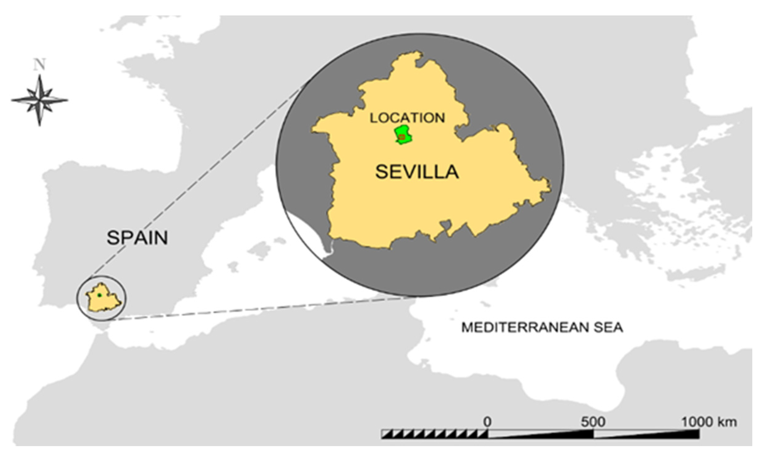
2.1. Mosaic of Cantillana
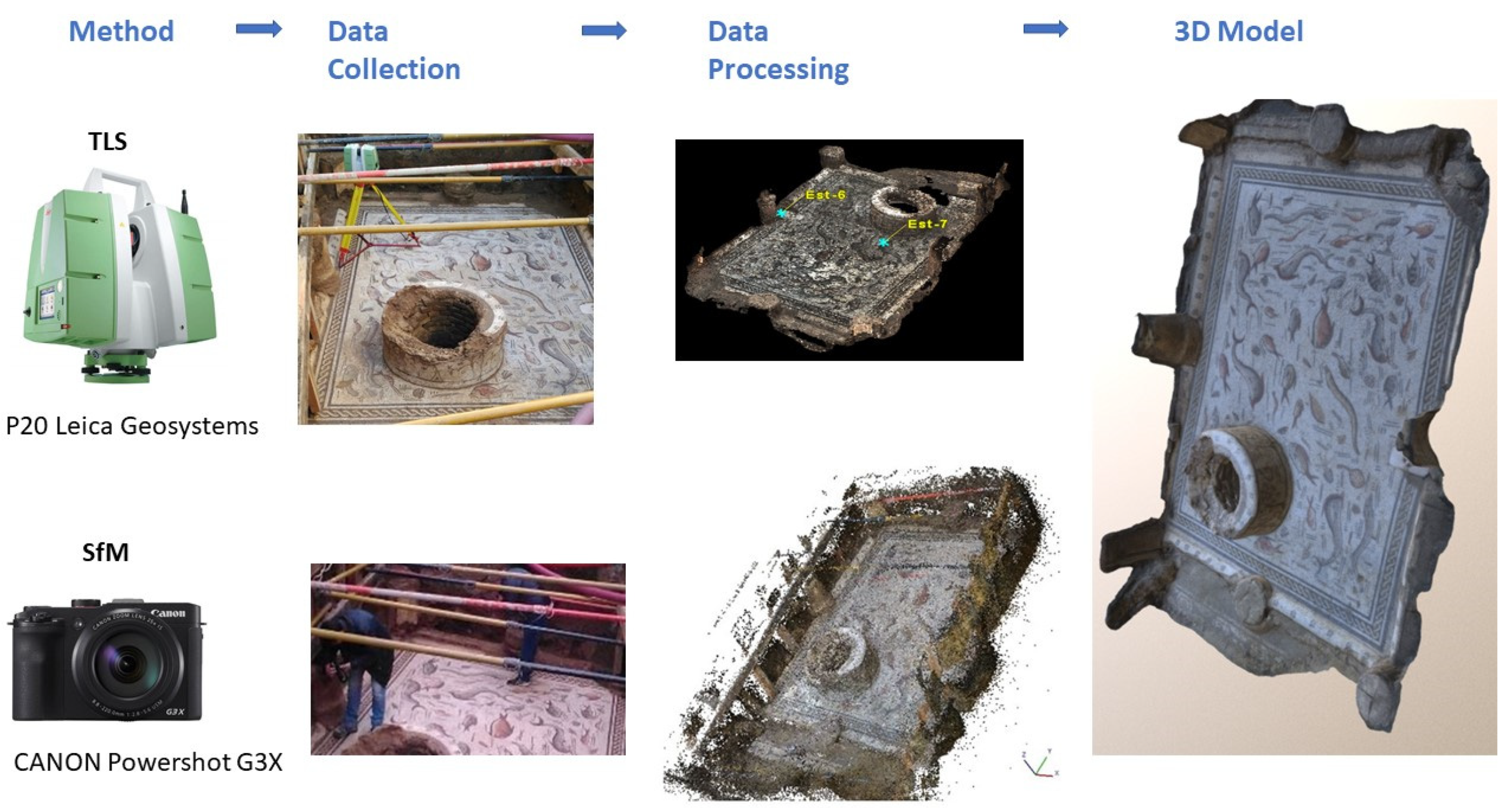
2.2. Methods
2.2.1. Georeferencing
2.2.2. Ground Control Points (GCP)
2.2.3. Photogrammetry (SfM)
2.2.4. Terrestrial Laser Scanning (TLS)
3. Results
3.1. SfM
3.2. TLS
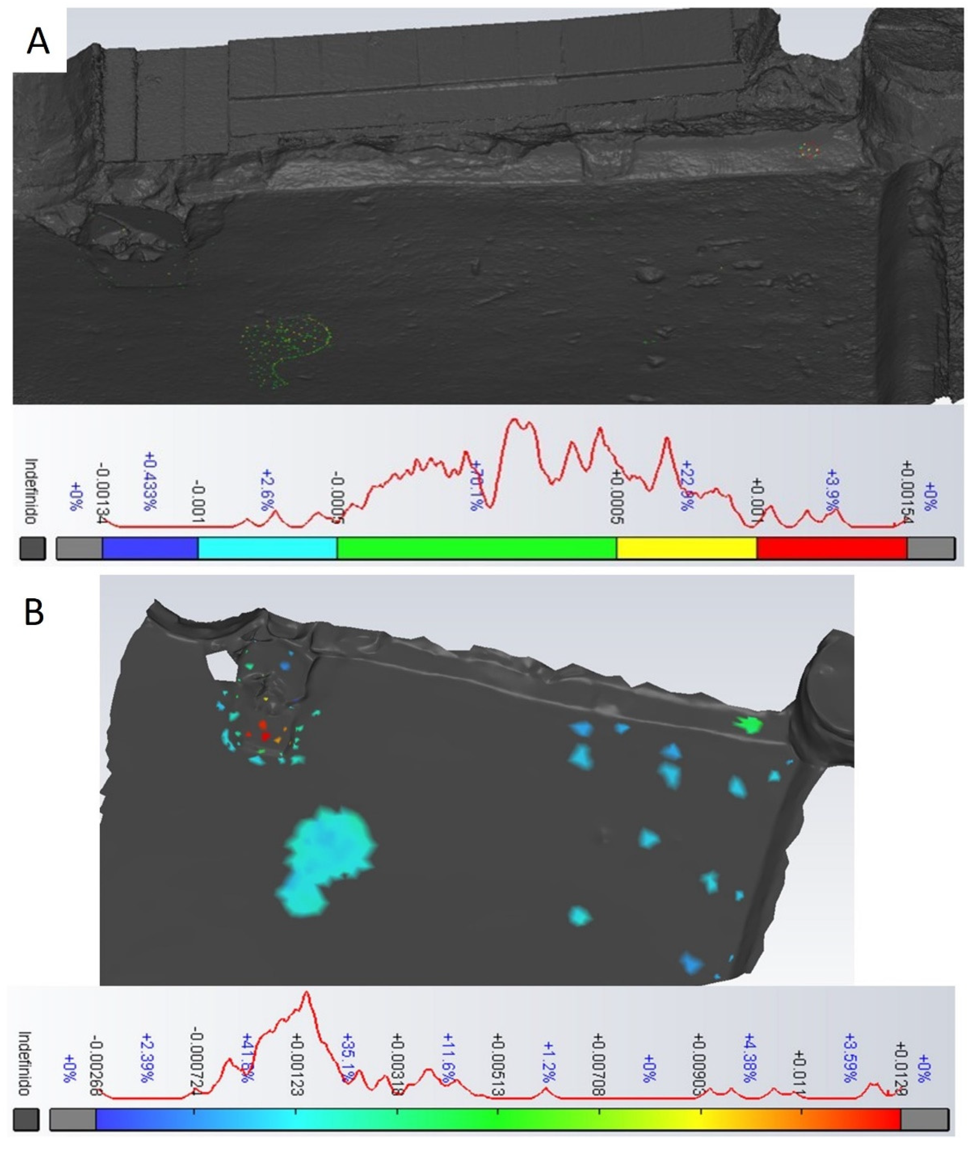
3.3. SfM vs. TLS
4. Discussion
5. Conclusions
Author Contributions
Funding
Institutional Review Board Statement
Informed Consent Statement
Data Availability Statement
Acknowledgments
Conflicts of Interest
References
- Marín-Buzón, C.; Pérez-Romero, A.; López-Castro, J.; Ben Jerbania, I.; Manzano-Agugliaro, F. Photogrammetry as a new scientific tool in archaeology: Worldwide research trends. Sustainability 2021, 13, 5319. [Google Scholar] [CrossRef]
- Cheng, L.; Chen, S.; Liu, X.; Xu, H.; Wu, Y.; Li, M.; Chen, Y. Registration of laser scanning point clouds: A review. Sensors 2018, 18, 1641. [Google Scholar] [CrossRef] [PubMed] [Green Version]
- Liang, X.; Kankare, V.; Hyyppä, J.; Wang, Y.; Kukko, A.; Haggrén, H.; Yu, X.; Kaartinen, H.; Jaakkola, A.; Guan, F.; et al. Terrestrial laser scanning in forest inventories. ISPRS J. Photogramm. Remote Sens. 2016, 115, 63–77. [Google Scholar] [CrossRef]
- Large, A.R.G.; Heritage, G.L.; Charlton, M.E. Laser scanning: The future. Laser Scanning Environ. Sci. 2009, 262, 262–271. [Google Scholar] [CrossRef]
- Gressin, A.; Mallet, C.; Demantké, J.; David, N. Towards 3D lidar point cloud registration improvement using optimal neighborhood knowledge. ISPRS J. Photogramm. Remote Sens. 2013, 79, 240–251. [Google Scholar] [CrossRef] [Green Version]
- Yang, B.; Dong, Z.; Liang, F.; Liu, Y. Automatic registration of large-scale urban scene point clouds based on semantic feature points. ISPRS J. Photogramm. Remote Sens. 2016, 113, 43–58. [Google Scholar] [CrossRef]
- Weinmann, M.; Hinz, S.; Jutzi, B. Fast and automatic image-based registration of TLS data. ISPRS J. Photogramm. Remote Sens. 2011, 66, S62–S70. [Google Scholar] [CrossRef]
- Puttonen, E.; Lehtomäki, M.; Kaartinen, H.; Zhu, L.; Kukko, A.; Jaakkola, A. Improved sampling for terrestrial and mobile laser scanner point cloud data. Remote Sens. 2013, 5, 1754–1773. [Google Scholar] [CrossRef] [Green Version]
- Kang, D.; Lee, H.; Park, H.S.; Lee, I. Computing method for estimating strain and stress of steel beams using terrestrial laser scanning and FEM. In Key Engineering Materials; Trans Tech Publications Ltd.: Freienbach, Switzerland, 2007; Volume 347, pp. 517–522. [Google Scholar] [CrossRef]
- Brechtken, R.; Przybilla, H.J.; Wahl, D. Visualisation of a necropolis on the basis of a portable aerial photogrammetric system and terrestrial laser scanning. In Proceedings of the ISPRS Congress Beijing 2008, Beijin, China, 3–11 July 2008; Volume XXXVII, pp. 667–672. Available online: https://www.researchgate.net/profile/Rainer-Brechtken/publication/242142584_VISUALISATION_OF_A_NECROPOLIS_ON_THE_BASIS_OF_A_PORTABLE_AERIAL_PHOTOGRAMMETRIC_SYSTEM_AND_TERRESTRIAL_LASER_SCANNING/links/5e4bbde6a6fdccd965af1d57/VISUALISATION-OF-A-NECROPOLIS-ON-THE-BASIS-OF-A-PORTABLE-AERIAL-PHOTOGRAMMETRIC-SYSTEM-AND-TERRESTRIAL-LASER-SCANNING.pdf (accessed on 11 December 2021).
- Boochs, F.; Kern, F.; Schütze, R.; Marbs, A. Approaches for geometrical and semantic modelling of huge unstructured 3D point clouds. Photogramm. Fernerkund. Geoinf. 2009, 2009, 65–77. [Google Scholar] [CrossRef]
- Lerma, J.L.; Navarro, S.; Cabrelles, M.; Villaverde, V. Terrestrial laser scanning and close range photogrammetry for 3D archaeological documentation: The Upper Palaeolithic Cave of Parpalló as a case study. J. Archaeol. Sci. 2010, 37, 499–507. [Google Scholar] [CrossRef]
- Grussenmeyer, P.; Landes, T.; Alby, E.; Carozza, L. High resolution 3D recording and modelling of the Bronze Age cave “Les Fraux” in Périgord (France). In Proceedings of the Conference ISPRS Commission V Symposium, Newcastle, UK, 2020; Volume 38, pp. 262–267. Available online: https://hal.archives-ouvertes.fr/hal-03099460/file/ISPRS_2010_Gruss_Land_Alb_Carozza.pdf (accessed on 11 December 2021).
- Lichti, D.D.; Gordon, S.J.; Stewart, M.P.; Franke, J.; Tsakiri, M. Comparison of digital photogrammetry and laser scanning. In Proceedings of the Proceedings: CIPA W6 International Workshop, Corfu, Greece, 1–2 September 2002; pp. 39–47. [Google Scholar]
- Fabris, M.; Achilli, V.; Artese, G.; Bragagnolo, D.; Menin, A. High resolution survey of phaistos palace (Crete) by Tls and terrestrial photogrammetry. Int. Arch. Photogramm. Remote Sens. Spat. Inf. Sci. 2012, 39, B5. [Google Scholar] [CrossRef] [Green Version]
- Peña-Villasenín, S.; Gil-Docampo, M.; Ortiz-Sanz, J. Professional SfM and TLS vs a simple SfM photogrammetry for 3D modelling of rock art and radiance scaling shading in engraving detection. J. Cult. Heritage 2018, 37, 238–246. [Google Scholar] [CrossRef]
- Blistan, P.; Jacko, S.; Kovanič, Ľ.; Kondela, J.; Pukanská, K.; Bartoš, K. TLS and SfM approach for bulk density determination of excavated heterogeneous raw materials. Minerals 2020, 10, 174. [Google Scholar] [CrossRef] [Green Version]
- Lewińska, P.; Róg, M.; Żądło, A.; Szombara, S. To save from oblivion: Comparative analysis of remote sensing means of documenting forgotten architectural treasures-Zagórz Monastery complex, Poland. Measurement 2021, 13, 110447. [Google Scholar] [CrossRef]
- Moyano, J.; Nieto-Julián, J.E.; Bienvenido-Huertas, D.; Marín-García, D. Validation of close-range photogrammetry for architectural and archaeological heritage: Analysis of point density and 3d mesh geometry. Remote Sens. 2020, 12, 3571. [Google Scholar] [CrossRef]
- Mohammadi, M.; Rashidi, M.; Mousavi, V.; Karami, A.; Yu, Y.; Samali, B. Quality evaluation of digital twins generated based on UAV photogrammetry and TLS: Bridge case study. Remote Sens. 2021, 13, 3499. [Google Scholar] [CrossRef]
- Verhoeven, G.; Doneus, M.; Briese, C.; Vermeulen, F. Mapping by matching: A computer vision-based approach to fast and accurate georeferencing of archaeological aerial photographs. J. Archaeol. Sci. 2012, 39, 2060–2070. [Google Scholar] [CrossRef]
- Méndez, V.; Pérez-Romero, A.; Sola-Guirado, R.; Miranda-Fuentes, A.; Manzano-Agugliaro, F.; Zapata-Sierra, A.; Rodríguez-Lizana, A. In-field estimation of orange number and size by 3D laser scanning. Agronomy 2019, 9, 885. [Google Scholar] [CrossRef] [Green Version]
- Villanueva, J.K.S.; Blanco, A.C. Optimization of ground control point (GCP) configuration for unmanned aerial vehicle (UAV) survey using structure from motion (SFM). Int. Arch. Photogramm. Remote Sens. Spat. Inf. Sci. 2019, 42. [Google Scholar] [CrossRef] [Green Version]
- Oniga, V.-E.; Breaban, A.-I.; Pfeifer, N.; Chirila, C. Determining the suitable number of ground control points for UAS images georeferencing by varying number and spatial distribution. Remote Sens. 2020, 12, 876. [Google Scholar] [CrossRef] [Green Version]
- Marín-Buzón, C.; Pérez-Romero, A.; Tucci-Álvarez, F.; Manzano-Agugliaro, F. Assessing the orange tree crown volumes using google maps as a low-cost photogrammetric alternative. Agronomy 2020, 10, 893. [Google Scholar] [CrossRef]
- Salaun, Y.; Marlet, R.; Monasse, P. Line-Based Robust SfM with Little Image Overlap. In Proceedings of the 2017 International Conference on 3D Vision (3DV), Qingdao, China, 10–12 October 2017; pp. 195–204. [Google Scholar]
- Cabo, C.; Del Pozo, S.; Rodríguez-Gonzálvez, P.; Ordóñez, C.; Aguilera, S.D.P. Comparing terrestrial laser scanning (TLS) and wearable laser scanning (WLS) for individual tree modeling at plot level. Remote Sens. 2018, 10, 540. [Google Scholar] [CrossRef] [Green Version]
- Marčiš, M. Quality of 3D models generated by SFM technology. Slovak J. Civ. Eng. 2013, 21, 13–24. [Google Scholar] [CrossRef] [Green Version]
- Truong-Hong, L.; Gharibi, H.; Garg, H.; Lennon, D. Equipment considerations for terrestrial laser scanning for civil engineering in urban areas. J. Sci. Res. Rep. 2014, 3, 2002–2014. [Google Scholar] [CrossRef]
- Large, A.R.; Heritage, G.L. Laser scanning–Evolution of the discipline. In Laser Scanning for the Environmental Sciences; Wiley-Blackwell: Oxford, UK, 2009; pp. 1–20. [Google Scholar]
- Lerma García, J.L.; Van Genechten, B.; Santana Quintero, M. 3D Risk Mapping. Theory and Practice on Terrestrial Laser Scanning. Training Material Based on Practical Applications; Universidad Politecnica de Valencia Editorial: Valencia, Spain, 2008; Available online: https://lirias.kuleuven.be/1773517?limo=0 (accessed on 11 December 2021).


| GCP | X | Y | Z | Edistance (mm) | Epixel |
|---|---|---|---|---|---|
| 1 | 250,501.239 | 4,165,808.807 | 30.225 | 1.7 | 0.352 |
| 2 | 250,503.802 | 4,165,808.644 | 30.201 | 0.9 | 0.285 |
| 3 | 250,504.121 | 4,165,808.976 | 30.199 | 0.7 | 0.175 |
| 4 | 250,504.042 | 4,165,806.570 | 30.134 | 0.6 | 0.313 |
| 5 | 250,504.003 | 4,165,805.965 | 30.148 | 3.6 | 0.265 |
| 6 | 250,503.921 | 4,165,804.518 | 30.208 | 1.5 | 0.424 |
| 7 | 250,501.001 | 4,165,804.747 | 30.251 | 0.6 | 0.559 |
| 8 | 250,500.937 | 4,165,805.000 | 30.252 | 08 | 0.308 |
| 9 | 250,503.342 | 4,165,807.727 | 30.177 | 04 | 0.213 |
| 10 | 250,501.945 | 4,165,807.384 | 30.204 | 04 | 0.198 |
| 11 | 250,502.596 | 4,165,806.482 | 30.185 | 24 | 0.289 |
| 12 | 250,503.031 | 4,165,804.971 | 30.201 | 15 | 0.463 |
| 13 | 250,502.005 | 4,165,805.997 | 30.748 | 02 | 0.275 |
| 14 | 250,502.448 | 4,165805.860 | 30.756 | 17 | 0.500 |
| 15 | 250,502.529 | 4,165805.234 | 30.747 | 15 | 0.600 |
| Target | X | Y | Z |
|---|---|---|---|
| D01 | 250,504.887 | 4,165,802.485 | 34.710 |
| D02 | 250,501.280 | 4,165,802.133 | 34.706 |
| D03 | 250,500.799 | 4,165,807.835 | 34.615 |
| D04 | 250,503.795 | 4,165,808.125 | 34.728 |
| Parameter | Value |
|---|---|
| Field of view | Full vault |
| Hz/V Area (°) | 90°/55° |
| Scan Mode | Scan Only |
| Resolution | 25.0 mm @ 10 m |
| Quality | 3 |
| Number of Dots (Hz × V) | 2514 × 1013 |
| Image Exposure | Auto |
| White Balance | Cold Light |
| Image Resolution | 1920 × 1920 |
| HDR Image | No |
| Estimated Time | 7 min 22 s |
| ≥5 mm | <5 mm | <2 mm | <1 mm | <0.5 mm | |
|---|---|---|---|---|---|
| GCP vs. SfM | - | - | 4.3% | 95.6% | 70.1% |
| GCP vs. TLS | 9.17% | 88.5% | 2.39% | - | - |
Publisher’s Note: MDPI stays neutral with regard to jurisdictional claims in published maps and institutional affiliations. |
© 2021 by the authors. Licensee MDPI, Basel, Switzerland. This article is an open access article distributed under the terms and conditions of the Creative Commons Attribution (CC BY) license (https://creativecommons.org/licenses/by/4.0/).
Share and Cite
Marín-Buzón, C.; Pérez-Romero, A.M.; León-Bonillo, M.J.; Martínez-Álvarez, R.; Mejías-García, J.C.; Manzano-Agugliaro, F. Photogrammetry (SfM) vs. Terrestrial Laser Scanning (TLS) for Archaeological Excavations: Mosaic of Cantillana (Spain) as a Case Study. Appl. Sci. 2021, 11, 11994. https://0-doi-org.brum.beds.ac.uk/10.3390/app112411994
Marín-Buzón C, Pérez-Romero AM, León-Bonillo MJ, Martínez-Álvarez R, Mejías-García JC, Manzano-Agugliaro F. Photogrammetry (SfM) vs. Terrestrial Laser Scanning (TLS) for Archaeological Excavations: Mosaic of Cantillana (Spain) as a Case Study. Applied Sciences. 2021; 11(24):11994. https://0-doi-org.brum.beds.ac.uk/10.3390/app112411994
Chicago/Turabian StyleMarín-Buzón, Carmen, Antonio Miguel Pérez-Romero, Manuel J. León-Bonillo, Rubén Martínez-Álvarez, Juan Carlos Mejías-García, and Francisco Manzano-Agugliaro. 2021. "Photogrammetry (SfM) vs. Terrestrial Laser Scanning (TLS) for Archaeological Excavations: Mosaic of Cantillana (Spain) as a Case Study" Applied Sciences 11, no. 24: 11994. https://0-doi-org.brum.beds.ac.uk/10.3390/app112411994