
Petri Net Toolbox for Multi-Robot Planning under Uncertainty


1
Institute For Systems and Robotics, Instituto Superior Técnico, University of Lisbon, 1049-001 Lisboa, Portugal
2
The MathWorks, Natick, MA 01760, USA
*
Author to whom correspondence should be addressed.
Appl. Sci. 2021, 11(24), 12087; https://0-doi-org.brum.beds.ac.uk/10.3390/app112412087
Submission received: 20 November 2021
/
Revised: 9 December 2021
/
Accepted: 10 December 2021
/
Published: 18 December 2021
(This article belongs to the Special Issue Recent Advances in Petri Nets Modeling)
Abstract
:Currently, there is a lack of developer-friendly software tools to formally address multi-robot coordination problems and obtain robust, efficient, and predictable strategies. This paper introduces a software toolbox that encapsulates, in one single package, modeling, planning, and execution algorithms. It implements a state-of-the-art approach to representing multi-robot systems: generalized Petri nets with rewards (GSPNRs). GSPNRs enable capturing multiple robots, decision states, action execution states and respective outcomes, action duration uncertainty, and team-level objectives. We introduce a novel algorithm that simplifies the model design process as it generates a GSPNR from a topological map. We also introduce a novel execution algorithm that coordinates the multi-robot system according to a given policy. This is achieved without compromising the model compactness introduced by representing robots as indistinguishable tokens. We characterize the computational performance of the toolbox with a series of stress tests. These tests reveal a lightweight implementation that requires low CPU and memory usage. We showcase the toolbox functionalities by solving a multi-robot inspection application, where we extend GSPNRs to enable the representation of heterogeneous systems and system resources such as battery levels and counters.
1. Introduction
Although the use of multi-robot systems has proven successful in a wide range of real life applications, coordinating these systems at mission-level is still challenging in a number of scenarios. Scientific competitions such as the DARPA subterranean challenge [1] and RoboCup [2,3] reflect the necessity of progress in this field. Despite the recent advances [4,5], a considerable amount of behaviors exhibited in these applications still achieve autonomy through hand-crafted rule-based plans [6,7] or sub-optimal optimizations [8]. These ad-hoc approaches require that a significant engineering effort is placed in every new scenario without even providing any type of formal guarantee on the deployed controllers. Furthermore, as the deployment scale grows, rule-based approaches tend to be harder to define and become more distant from the optimal behavior. In some cases this also leads to many exposed design flaws that have been raising concerns about the safety and reliability of autonomous systems [9,10].
So far, the most common approach to tackle this problem is through exhaustive testing. This brute-force approach does not produce results as good as formal methods when comparing aspects such as efficiency, robustness, reliability, safety and predictability [11,12]. Thus, formal methods for synthesizing plans for autonomous systems, have proven to be a successful approach to tackle these concerns. However, the lack of developer-friendly software tools that implement these methods is hindering their adoption. In this work, we introduce a software toolbox that allows: modeling multi-robot systems taking into account time uncertainty; obtaining coordination strategies that guarantee optimality; and executing these strategies in the Robot Operating System (ROS) environment. The proposed software provides methods that capture system constraints by design, provide algorithms to analyze the obtained plans before execution, and execute them in real robots.
Despite the existence of software tools and libraries to model, extract optimal policies and coordinate the execution of multi-robot systems, they were developed and implemented separately and are not interoperable. Moreover, none of them assembles in the same tool the capability of capturing stochastic behavior along with methods to synthesize and execute optimal policies that take into account such uncertainty.
PRISM [13] and STORM [14] are open source probabilistic model checkers, that support discrete and continuous time Markov chains, Markov decision processes (MDPs) and generalized stochastic petri nets (GSPNRs). Both these tools allow model analysis, providing reachability properties, conditional probabilities and cost queries, long-run average values, cost-bounded properties and multi-objective queries. However, they are not built specifically for robotic systems and do not allow policy execution.
Similarly to PRISM and STORM, Pipe [15] and GreatSPN [16] allow the modeling of Petri nets and provide multiple analysis algorithms that yield logic and performance properties. Moreover, it provides a user-friendly graphical interface to build such models, which reduces the entry barrier for first users and facilitates the modeling step. Still, it does not provide policy synthesis methods neither robot coordination capabilities, through policy execution.
Robot coordination under ROS middleware is usually achieved using SMACH [17]. SMACH provides an approach based on nested state machines that has proven effective at building and executing task plans with real robots. Though one of the reasons for the popularity of SMACH is its simplicity, making it restrictive in many applications. Thus SMACH does not provide elements to model uncertainty and stochastic effects that are often present in real robot tasks. Furthermore, it is not able to choose from alternative set of actions, that is a necessary feature to produce policies for the designed models.
Finally, Petri Net Plans [18] is the software tool closest to the one proposed in this work. It allows coordination of single and multi-robot systems through task plans designed as Petri nets. It is integrated with ROSPlan [19] and executes the task plans using actionlib. However, it is less scalable as it uses one Petri net model per represented robot. It also does not provide methods to capture probabilistic behavior, or supports policy synthesis and, consequently, requires the input of a task plan.
Our work addresses these gaps and proposes a unified toolbox to implement multi-robot coordination problems. This toolbox allows us to capture multi-robot systems as a generalized stochastic Petri net with rewards (GSPNR) [20], to synthesize optimal control policies that optimize team-level objectives, and provides methods to execute the obtained task plans in real robots. GSPNRs allow for unified modeling of action selection, uncertainty on the duration of action execution, and for goal specification through the use of transition rewards and rewards per time unit. When compared against traditional multi-robot formalisms, such as multi-agent Markov decision processes (MMDPs) [21], GSPNRs provide: better scalability and fully asynchronous execution, ensuring a smaller state-space and a more fluid policy execution. This work introduces also a novel algorithm to build GSPNR models from a topological map. This is an intuitive and quick method to design complex models especially for users that are not comfortable with manipulating GSPNRs. It also provides a novel execution algorithm that is able to coordinate robots through ROS. GSPNRs for multi-robot systems is an efficient representation since it models robots as indistinguishable tokens. The proposed execution algorithm is able to track each individual robot, and distinguish between them without compromising the state space efficiency. We provide a rigorous characterization of the toolbox, namely the algorithms’ complexity and the computational resources required as the modeled system increases in complexity. Finally, we address a solar farm inspection problem where the capabilities of the toolbox are showcased. When solving this problem we introduce an extension to the work in [20] to enable modeling heterogeneous multi-robot systems and system resources such as battery levels and counters.
2. Background
Generalized stochastic Petri nets [22] extend Marked Ordinary Petri nets (MOPNs) by adding the capability of modeling events that take a stochastic time until completion. In [23] we introduced GSPNs with rewards that extend GSPNs by adding place and transition rewards. A GSPNR for multi-robot systems is a tuple and is defined as follows:
- P is a non-empty and finite set of places that models local robot states. These represent action execution or action selection states for subsets of the multi-robot system, denoted as action places and decision places, respectively;
- is a finite set of transitions partitioned into the subset of all immediate transitions and of all timed transitions . The firing delays of timed transitions are exponentially distributed and model the time uncertainty associated with these uncontrollable events, such as the time a robot takes to traverse the path between two locations. The immediate transitions represent the controllable actions that the team of robots has available;
- and are input and output arc weight functions, respectively. Input arcs assign which timed events can trigger or what are the available actions in a local state. Output arcs dictate the local state update resulting from such timed events or of the selected action;
- is a function that associates a rate to each timed transition or a weight to each immediate transition, dictating the probability distribution of the uncontrollable events or of the control policy, respectively;
- is the initial marking. A marking represents the number of robots executing each action or in each decision state;
- is the place reward function and gives a reward per time unit in markings where there is at least one token in p;
- is the transition reward function and gives a reward every time the action, associated to is selected.
In this representation each token corresponds to an individual robot. The marking represents the global state of the system, where means that there are k robots in the local state represented by . The dynamics of a GSPNR is defined by the firing rule, which determines how the robots move from the execution of one action to the next and how the action selection impacts the local states of the robots. The firing rule dictates that when one transition t is fired tokens are consumed from all the places that have input arcs to t and tokens are produced in all the places that have output arcs from t. Transitioning from marking m to marking due to the firing of t is denoted as .
The set that contains all markings reachable from the initial marking , under the firing rule, is denoted as . The reachable state space of a conservative GSPNR has an upper bound given by the number of multisets of cardinality , with elements taken from a finite set of cardinality . We shall refer to this as p multichoose r, where and . We denote the set of input places of transition t as .
A marking where at least one immediate transition is enabled is denoted as vanishing. A marking where there are no immediate transitions enabled and there is at least one timed transition enabled is denoted as tangible. The set of all vanishing markings and the set of all tangible markings are denoted as and , respectively. In a tangible marking the total transition frequency from m to the output marking is given by:
where is the set of all transitions that move the system from m to . The exit frequency of a tangible marking is defined as:
Figure 1 (Left) depicts the topological map of a multi-robot navigation scenario and Figure 1 (Right) shows one possible GSPNR model that captures this problem. The three locations are represented by the places , and . The immediate transitions, here depicted as black rectangles, represent action selection. In each robot has two alternatives: move to or move to ; while in and the robots only have one alternative: move to . Selecting one navigation action (e.g., ) triggers its execution. Action execution is captured by the places that these immediate transitions lead to. The timed transitions, here represented as white rectangles, capture the uncertainty in the duration of the navigation actions. So, for example, if traversing takes longer than traversing , the rate of the timed transition will be inferior to the rate of the timed transition . Each token represents an individual robot and this allows to add or remove robots from the multi-robot system without changing the structure of the GSPNR model. In this example, there are two robots in as the current marking shows.
3. Materials and Methods
This section describes in detail the implemented toolbox that provides in a single toolbox methods that enable modeling, policy synthesis and plan execution in multi-robot systems.
3.1. Toolbox Overview
The toolbox functionalities are organized into three modules as depicted by the architecture in Figure 2. The model design module implements methods to capture, as a GSPNR model, multiple robots, decision states, action execution states and respective outcomes, action duration uncertainty, robot resources, and team-level objectives. Furthermore, it provides model simulation methods that allow to assess the multi-robot system behavior when following a provided policy. This provides insight on the designed model and policy before executing it in ROS. The policy synthesis module provides planning algorithms that optimize the total expected reward and the discounted expected reward gathered by the multi-robot system as a whole. Finally, the execution manager module implements execution algorithms that coordinate the multi-robot system according to a provided policy. This is achieved via an interface between the toolbox and ROS that is implemented in this module.
This toolbox is implemented in MATLAB®, is open source and available at [24]. To install it, the user has to clone the repository to its own computer and run the install.m file. This will lead to a Getting Started live script that guides the user through a series of tutorials that cover the main functionalities of the toolbox with illustrative examples. The next subsections describe in detail each of the modules that comprise the toolbox.
3.2. Model Design
The model design module allows abstracting the multi-robot dynamics and the world interaction as a GSPNR model. It provides three different methods to capture it: a manual and unconstrained design method to build the GSPNR model; a model composition method that automatically builds the GSPNR from a topological map; and a method that imports from third-party tools the designed Petri net and converts it to a GSPNR.
The first method allows to design programmatically every element of the GSPNR tuple. It does this by implementing the GSPNR formalism, as defined in Section 2, as a MATLAB® class, and thus exposing a simple API that provides methods to add or remove: tokens, places, transitions, arcs and reward functions. This input method provides freedom to create any kind of model but it requires a deeper knowledge on GSPNRs. Therefore, it is recommended for more experienced users.
The code snippet below shows how to use the API to manually design the GSPNR model depicted in Figure 1 (Right). The methods, add_places, add_transitions and add_arcs, are self-explanatory and allow adding places, transitions and arcs, respectively. The number of tokens in each place are added at the same time the places are created. The place and transition rewards are set with the set_reward_functions method. The user must specify the reward value and the place or transition that triggers that reward. When a place reward is added, the system will receive the reward value per unit of time as long as there is more than one token on that place. The transition reward is received every time the transition is fired. For explanatory reasons this snippet of code is exhaustive an enumerates every single place and transition names. However, the number of lines can be reduced using for-loops and by carefully choosing names that overlap.
| % instantiate model |
| gspnr_model = GSPNR(); |
| places = [“L1”, “L2”, “L3”, “NavigatingL1-L3”, … |
| “NavigatingL3-L1”, “NavigatingL1-L2”, … |
| “NavigatingL2-L1”]; |
| tokens = [2, 0, 0, 0, 0, 0, 0]; |
| % add places |
| gspnr_model.add_places(places, tokens); |
| transitions = [“GoL1-L3”, “GoL3-L1”, “GoL1-L2”, “GoL2-L1”, … |
| “ArrivedL1-L3”, “ArrivedL3-L1”, “ArrivedL1-L2”, “ArrivedL2-L1”]; |
| types = [“imm”, “imm”, “imm”, “imm”, “exp”, “exp”, “exp”, “exp”]; |
| rates = [0, 0, 0, 0, 0.1, 0.1, 0.05, 0.05]; |
| % add transitions |
| gspnr_model.add_transitions(transitions, types, rates); |
| arc_places = [“L1”,“NavigatingL1-L3”, “NavigatingL1-L3”, “ArrivedL1-L3”, “L3”, … |
| “NavigatingL3-L1”, “NavigatingL3-L1”, “L1”, “L1”, “NavigatingL1-L2”, … |
| “NavigatingL1-L2”,“ArrivedL1-L2”,“L2”,“NavigatingL2-L1”,… |
| “NavigatingL2-L1”,“L1”]; |
| arc_transitions = [“GoL1-L3”, “GoL1-L3”, “ArrivedL1-L3”, “L3”, “GoL3-L1”,… |
| “GoL3-L1”, “ArrivedL3-L1”, “ArrivedL3-L1”, “GoL1-L2”,… |
| “GoL1-L2”, “ArrivedL1-L2”, “L2”, “GoL2-L1”, “GoL2-L1”,… |
| “ArrivedL2-L1”, “ArrivedL2-L1”]; |
| arc_type = [“in”, “out”, “in”, “out”, “in”, “out”, “in”, “out”, “in”, “out”, “in”, … |
| “out”, “in”, “out”, “in”, “out”]; |
| arc_weights = [1, 1, 1, 1, 1, 1, 1, 1, 1, 1, 1, 1, 1, 1, 1, 1]; |
| % add arcs |
| gspnr_model.add_arcs(arc_places, arc_transitions, arc_type, arc_weights); |
| reward_names = [“NavigatingL1-L3”, “GoL1-L3”]; |
| reward_values = [1, 5]; |
| reward_types = [“place”, “transition”]; |
| % set reward function |
| gspnr_model.set_reward_functions(reward_names, reward_values, reward_types) |
For more inexperienced users, manually building complex models using the API can be a cumbersome task. In order to address this issue, and steepen the toolbox learning curve, the GSPNR module implements an algorithm that automates model composition. This allows building an extended GSPNR model from template models automatically, and thus, simplifies the design process. These template models capture the primitive actions the system can perform and, as a result, we shall call them action models. The automated model composition is detailed in Algorithm 1. This algorithm produces as output an extended GPSNR and takes as input:
- (1)
- The topological map that the robots will use to navigate. This must be a directed topological map with nodes, directed edges and weights that can optionally be assigned to edges. These edge weights represent the average time to travel between the two connecting nodes.
- (2)
- A function , where is a set with all the topological map nodes and edges. is a set with all the actions that the system can execute, modeled as GSPNRs. Thus, this function specifies the action models that the system can perform in each topological map node plus the navigation action that is executed when traversing the edge between two nodes.
- (3)
- A vector that contains the starting node of each robot in the topological map.
| Algorithm 1 Algorithm that builds an extended GSPNR from action models and a topological map. |
input: , , output:
|
Overall, Algorithm 1 replicates and merges, for each topological map node and edge, the action models provided by the function. This is visible in the code blocks in lines 1–16 and 17–34. First, the algorithm goes through all the nodes of the topological map adding and merging the action models of each action available in that node. Then, it connects the action models in each node using the navigation action model defined for each edge. The navigation action model is mandatory when there is more than one node in the topological map. The places with the same name are merged into one single place and the transitions are redirected to it.
The function defines the actions that can be executed in each node and edge of the topological map. These actions are typically identical across all the topological map. Still, the extended GSPNR model must be able to distinguish when the same action is executed in different regions of the topological map. Thus the algorithm adapts the action models for each node and edge on the topological map. This ensures that the same action on different locations is captured with different names whilst only requiring the manual design of a single model per action. To achieve this the user should use the special symbols on the places and transitions names of the designed actions. These angle brackets are used by the algorithm and replaced by the respective node name as defined in lines 5–6 and 21–22 of Algorithm 1. When replacing the angle brackets in edges the algorithm uses the names of the source and target nodes. Consider a place named Navigating – that is part of the navigation action model. This place is renamed to Navigating – for the edge connecting Node A to Node B and renamed to Navigating – for the edge connecting Node A to Node C.
Additionally, the navigation action may take more or less time to execute depending on the region of the topological map where it is being performed. The user can define the duration uncertainty of traversing each edge without designing a different navigation model for each edge. To do this the user must assign a weight to each topological map that should correspond to the average duration of traversing that edge. Algorithm 1 assumes that there is a single timed transition that models the edge traversing uncertainty and sets the rate of that transition to the reciprocal of the edge weight as detailed in line 24.
The algorithm also sets the initial state of each robot. This is done by setting the initial marking of the extended GSPNR . As it is detailed in lines 35–37, the algorithm adds one token to the place that has the same name as the node where the robot will start. This place was already created when iterating through all the topological map nodes in lines 1–16. The initial node of each robot is provided by the user as the vector. This vector does not require a particular order due to the homogeneous nature of the multi-robot system. Nevertheless if two or more robots start in the same node, this node should be repeated in the vector.
Note that the pseudocode detailed in Algorithm 1 is a simplification of the actual implementation. The real implementation, available here [24], checks for wrong inputs and prevents the algorithm from outputting a GSPNR with missing elements. Moreover, instead of the function the user can input a simpler function that only specifies the action names that can be executed in each node of the topological map. In this case, the algorithm uses a template action model identical to the one depicted in Figure 3 and replaces the action name for the one provided in .
This lifts the need to understand the GSPNR formalism, and expands the toolbox userbase to a group of users that does not require complex GSPNR models to capture multi-robot systems.
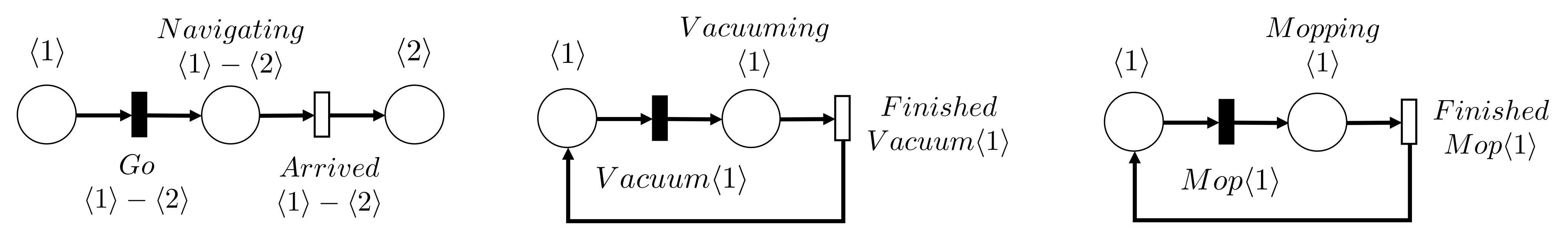
To better understand how model composition algorithm works consider the multi-robot navigation example presented in Section 2. Consider that each robot, besides navigating, can also vacuum and mop each location. These are the three actions that the multi-robot system can perform and that need to be modeled. Figure 3 (Left), Figure 3 (Center) and Figure 3 (Right) shows the primitive actions GSPNR model for navigation (), vacuuming () and mopping (), respectively. The brackets allow defining how the places and transitions names should change from one location to the other. These brackets will then be replaced by the names given to the topological map nodes. In this example, the function sets the same actions for all nodes, so . It also sets a single navigation model for all the edges, so . The navigation duration uncertainty in each of these edges is defined by the weights in the topological map. Assume that the arc weight and is 10 and the arc weight of and is 20, because on average it takes 10 min to traverse and 20 min to traverse . Then the transitions and have an rate and the transitions and have an rate. Figure 4 shows the extended GSPNR, that originates from inputting the models in Figure 3 and the topological map in Figure 1 (Left). In this case, since we have a multi-robot system with two robots starting in location . The reward function must then be defined using the API method set_reward_functions.
Finally, the user can also design the GSPNR model using third-party tools. This is enabled by import and export methods that interface this tool with Pipe [25] and GreatSPN [16]. These third-party provide access to a GUI that may prove to be more intuitive for beginners. It also enables analysis of behavioral, structural and time-dependent properties that both these tools implement. These analysis may help find errors in the designed models such as the presence of unwanted deadlocks or boundedness noncompliance. Despite this, the user will always have to resort to our toolbox API to add the reward functions, since at the present time these third-party tools do not provide mechanisms to do it. This approach is restricted to simple models, since as model complexity grows the graphical representation of the GSPNR becomes cluttered and difficult to manipulate and understand.
To capture the uncertainty present in some system wide properties, such as battery discharge, we introduce a change to the GSPNR formalism presented in Section 2. We partition the set of immediate transitions into two mutually exclusive subsets: a set of controllable actions and a set of uncontrollable immediate transitions . The controllable action set keeps the same semantics and usage as the original set and so each transition is viewed as an independent selectable action with a deterministic outcome. The transitions in are viewed, for a given marking, as a single action with a stochastic outcome. This means that, in a given marking, all enabled immediate transitions that belong to form a random switch. Thus the weights assigned to these transitions define the probability distribution that captures the system property in question. Thus, if in that same marking there are other immediate transitions that belong to these are taken as individual action selection and do not form a random switch. The random switch is a single action, that we shall denote as ⊤, with a stochastic outcome defined by the weights of each . So, in marking , the probability of transition is given by: , where is the set of all enabled uncontrollable immediate transitions.
3.3. Policy Synthesis
The policy synthesis module provides algorithms to synthesize optimal policies that optimize team-level objectives. The diagram in Figure 5 shows the implementation of the policy synthesis method. This method takes as input the GSPNR model built with the design module and outputs the optimal policy . The optimal policy is defined as . The ⊥ action represents all uncontrollable timed actions that in are viewed as timed transitions. The ⊤ action represents transitions with an uncertain outcome and selecting it means triggering the formed random switch. In the , these are viewed as uncontrollable immediate transitions. The policy defines for each marking what is the optimal action to select. In a nutshell, the algorithm converts into an equivalent MDP and then applies value iteration. The obtained policy is then mapped from the MDP states to the GSPNR markings, yielding the policy [20].
The policy synthesis algorithm optimizes team-level objectives that are influenced by the defined reward functions and by the performance objective selected. This module implements two performance objectives: the total expected reward objective, defined as:
and the discounted expected reward given by:
where denotes the control policy, the state distribution, r the reward function, t the time step and the discount factor. The objective takes into account the total reward value accumulated, however it is restricted to scenarios with finite horizons. The converges even in infinite horizon scenarios, since it discounts future rewards, giving more weight to the rewards received in the initial markings.
In order to find the optimal policy that optimizes such objectives the GSPNR model is converted to an equivalent MDP. Let be a GSPNR. Let be the maximum rate among all tangible markings and be a normalization constant.
The equivalent MDP obtained from is defined as , where: , that is, the state space is comprised by all the reachable markings of ; , that is, the initial state corresponds to the initial marking in ; , that is, the set of actions includes all controllable immediate transitions, plus the action ⊥ and the random switch ⊤; the transition probability is given by:
The reward function is defined as:
where represents the set of places with at least one token in a given marking, and is the set of all enabled uncontrollable immediate transitions as defined in Section 3.2.
The existence of an equivalent MDP for the GSPNR enables the use of dynamic programming solvers to obtain the optimal policy. In this case we implement value iteration [26]. The yielded optimal policy dictates which actions should be taken in each state, and, in the GSPNR, this corresponds to selecting an immediate transition for each marking and is defined as . As the GSPNR to MDP conversion algorithm explores the GSPNR reachability graph it also builds a function that allows mapping the equivalent MDP states back to GSPNR markings. This function, defined as , sets which state in corresponds each marking in . It enables the conversion from the optimal policy obtained in the MDP, , to the optimal policy in the GSPNR, . Thus, the optimal policy in the GSPNR is defined as .
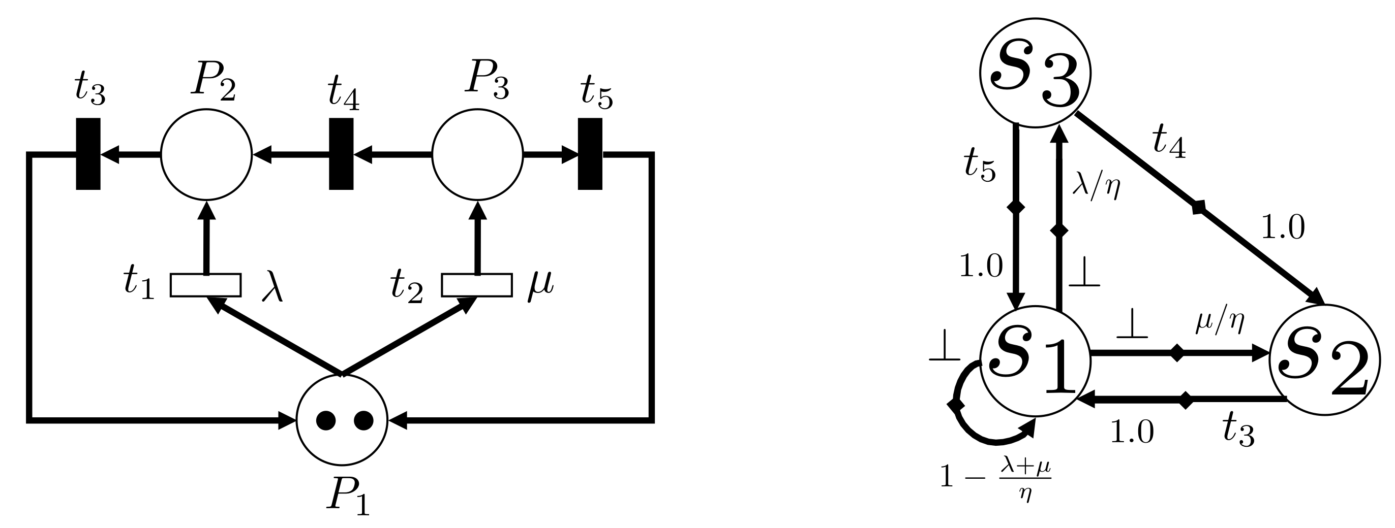
Figure 6 shows an example of the GSPNR to MDP conversion, where , and . Consider that the reward function gives a reward of 1 in place and zero everywhere else. Thus, value iteration will output the following optimal policy: , and . Finally, the function allows mapping into . The policy in state and state has a direct correspondence. In the action ⊥ represents waiting for the outcome of executing action , that is, waiting for the uncontrollable event or to trigger.
The obtained policy is optimal in the designed GSPNR model. Thus, it is limited by how well the model captures reality. So inaccurate models may lead to erroneous policies that produce unwanted behaviors. To detect these issues, before moving to the real scenario deployment, this toolbox provides a model simulation method implemented under the evaluate_policy() API function. The model simulation is a Monte Carlo based method that samples from the model by firing transitions and progressing through the state space collecting timestamps. It provides the states, actions selected, and the duration of each action during the simulated horizon. The simulation horizon is given by the user as the amount of time in seconds that the simulation should run. The immediate transitions are fired according to the given policy and the timed transitions according to the exponential distribution generated from their rates. The user can then compute, from the simulation data, multiple properties that help evaluating the policy performance and the model correctness. For instance, it can assess: the mean time to reach a certain state; the mean time spent in each state; the probability of reaching a certain state within a given horizon; the average throughput of a certain action; the average number of robots in each action or decision state; or how the robot probability distribution per action or decision state evolves over time. Even when the model is correct this can be used to make it more efficient and realistic through the analysis of how changes in the GSPNR model affect these properties. On top of that, it is possible to simulate a high number of states and transitions in a short amount of time since the method does not need to actually wait for the actions to execute.
3.4. Execution Manager
The execution manager module coordinates the multi-robot system and guarantees that the task is executed according to the designed GSPNR model and the provided policy. The GSPNR model alone is not enough to have an executable task plan since the GSPNR has non-determinism necessary for the action selection process. Applying a given policy to the GSPNR model resolves this non-determinism and enables the task plan execution.
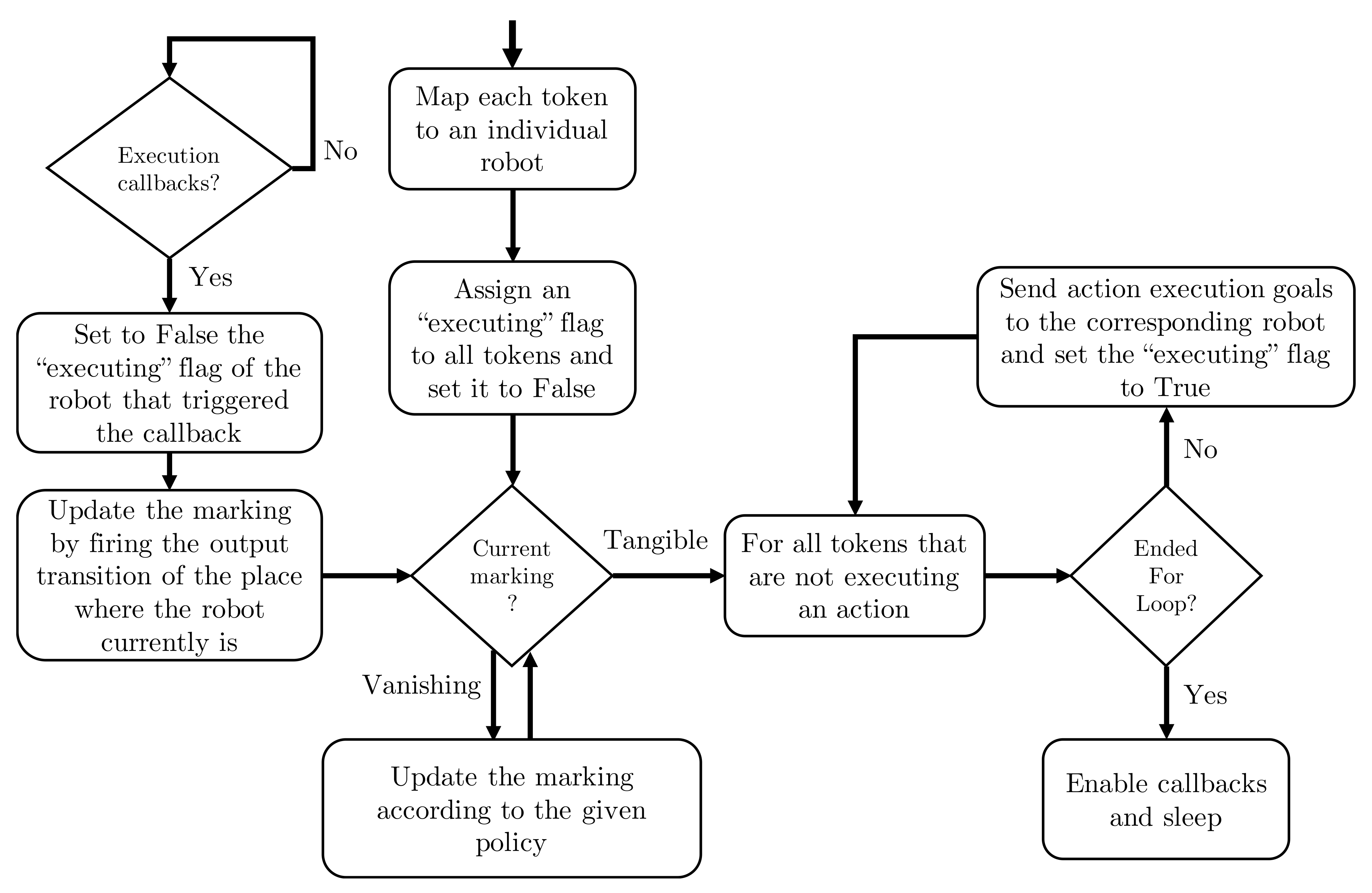
Figure 7 shows a flowchart that summarizes the execution manager module algorithm. This module is able to coordinate real systems as it interfaces with ROS actionlib through the MATLAB® ROS Toolbox. The coordination algorithm takes four inputs:
- 1.
- GSPNR model ;
- 2.
- policy ;
- 3.
- mapping function between each robot’s identifier and its initial GSPNR place;
- 4.
- mapping function between each action place and the respective ROS ActionServer.
The robot identifier must be the robot’s ROS namespace. The algorithm assumes that the ROS packages of different robots are launched under different namespaces, and the packages of the same robot are launched under the same namespace. The must specify the action server name, the package name, the action name and the message fields for each action place. This mapping can be inputed as a YAML configuration file or using a MATLAB® structure array.
The algorithm runs until it reaches a terminal marking or until the process is killed, and is executed as follows. First it establishes the correspondence between each token in the and each individual robot in the multi-robot system using . This ensures that the system knows in every marking which robot should be performing which action. Then it checks if the current marking of is vanishing or tangible. A vanishing marking is an action selection state while a tangible marking is an action execution state. Thus when in a vanishing marking it applies the given policy until it lands in a tangible marking. Applying consists in firing the immediate transition prescribed by for that given marking. This step takes a negligible amount of time when compared with action execution. When in a tangible marking it sends actions goals to all the robots that are not executing any action. To do this it gets the ActionServer name from according to the robot’s current place. Then it sends the goal to that ActionServer with the message fields also provided in . Once one robot finishes executing its action the algorithm fires the output timed transition that is connected to the place where the robot token currently is. This leads to a new marking and the process repeats again.
The novel feature of the execution manager algorithm is being able to provide an accurate mapping between robots as these are represented as indistinguishable tokens in the GSPNR. The algorithm first maps the actions each robot is executing to places in the Petri net. This is done by looking at the user provided configuration file that specifies, for each action place, which action server should be executed. By doing this, the algorithm assigns to each robot one token according to the action that each robot is currently executing. If two or more robots are executing the same action, the algorithm randomly maps the tokens in that action place to those robots. In this case, it is not necessary to distinguish between those robots, since we assume that heterogeneous robots can never share the same action place. Once the current action being executed finishes, the marking evolves until a new action must be executed. During this, the algorithm tracks each token, ensuring the correct mapping to each robot.
The execution manager algorithm is implemented in centralized manner, where one of the robots or an external machine runs MATLAB® and the execution algorithm. This allows for the coordination of robots with low computational resources, since the control and coordination algorithms (for navigation, localization, etc.) can run in a separate machine given that it stays inside the same network. Furthermore, the implemented algorithm is fully asynchronous, that is, it sends a new action goal as soon as one robot finishes the current execution. This is possible due to asynchronous nature of the Petri net formalism, in contrast with multi-agent MDPs that require that all robots finish the current execution to issue new actions. Finally, the execution manager is compliant with ROS1 enabling a more immediate impact in the community since currently there are many packages that are yet to migrate to ROS2.
3.5. Computational Performance and Scalability
To evaluate the toolbox’s computational performance we performed a series of tests for each module. All these tests are built using the same multi-robot scenario. We considered a generic problem with a linear topological map where each node is connected to the next one and the previous one. The first and the last node are only connected to the next or the previous node, respectively. The robots can navigate in this topological map and in each node can execute two different actions: Action A and Action B. Every action has a different duration uncertainty, and so it is defined by a different rate. The GSPNR that models this problem is similar to the one depicted in Figure 4, with the difference that was adapted for a topological map with a linear topology.
The results were obtained in a machine with an i74690 CPU, 32GB of RAM and a NVIDIA RTX 2080 Super GPU. The CPU measurements were taken in relation to the usage of a single core. Thus, 100% usage means one CPU core being fully used, 200% corresponds to two CPU cores fully used, and so on.
The first test measured the average time required by Algorithm 1 to generate a GSPNR model from a given topological map. Figure 8 (Left) and Figure 8 (Right) show the results obtained as the number of locations and the number of robots grows, respectively. These results show that the time to build the GSPNR model grows quadratically with the number of locations and is constant as the number of robots grows. The Algorithm 1 iterates over all the nodes and then over all the edges. For a topological map with a linear topology the number of edges is , where n is the number of nodes. Inside each of these loops the algorithm has to merge the newly created action model with the existing GSPNR model. This requires looping through all places and transitions and these elements grow linearly with the number of nodes. So this leads to a computational complexity of , where n is the number of nodes in the topological map. A further analysis of the Algorithm 1 shows that the computational complexity depends on the average degree of the topological map. For a fully connected topology the number of edges is and this means that the computational complexity of the Algorithm 1 is . Increasing the number of robots does not increase the number of iterations necessary to build the GSPNR. This arises from the fact that the algorithm only needs to iterate over all the nodes and for each node add the total number of robots in that location. Increasing the number of robots does not change the number of nodes on the topological map and therefore the generation time remains constant. Thus, the algorithm has a computational complexity of in this case. The computational complexity of the Algorithm 1 is coherent with the results shown in Figure 8.
The second test assesses how the policy synthesis module scales. Figure 9 (Left) and Figure 9 (Right) shows how the state space of the equivalent MDP grows as the number of locations and the number of robots increases, respectively. For a conservative GSPNR with p places and r tokens, the reachable markings upper bound is given by p multichoose r. In Figure 9 the growth is slightly slower than p multichoose r, since the way the GSPNR model was designed restricts some parts of the state space. Alternative approaches, such as MMDPs [21] or designing a single Petri net for each robot [27], grow faster. These alternatives follow a growth of where p is the number of state factors in the MMDPs and r the number of robots. Intuitively this can be explained by the fact that alternative approaches keep a state factor for each robot, whereas GSPNRs for multi-robot systems only count the number of robots in each state.
The method to obtain the optimal policy requires converting the GSPNR model to an equivalent MDP and then applying value iteration. Figure 10 (Left) shows the time required by these two components as the GSPNR state space increases, with a convergence error of and a discount factor of . The amount of time the value iteration algorithm takes to converge is one order of magnitude greater than the time it takes to obtain the equivalent MDP. However, the amount of time required for the value iteration to converge depends on the convergence error, the discount factor and the reward function. To isolate the evaluation from those factors it is measured the average time of each iteration, as Figure 5 (Right) shows. This indicates that the iteration time increases quadratically with the number of states. This stems from the fact that value iteration algorithm loops over all the states and then for each action loop over all the possible outcome states.
Figure 11 shows the computational resources required as the model complexity increases, when executing the obtained task plan in ROS. The goal was measuring the resources required by the execution module alone. Thus, the two actions (Action A and Action B) that each robot can execute in each location were implemented as mockup action servers. These action servers simply sleep during a predefined amount of time and then return success. Increasing the number of robots means having more action servers running in parallel as an instance of each action server is launched per robot. Increasing the number of locations does not affect the number of action servers, but increases the size of the GSPNR model as more places and transitions are required to capture a bigger topological map. The results show a negligible average CPU usage and a memory usage near 0.9 GB. They also show that these values remain constant when increasing the problem complexity. The memory usage of the proposed toolbox is one order of magnitude lower when comparing with equivalent MMDPs or state machines implementations. This discrepancy yields from the fact that the GSPNR formalism defines the rules to generate the reachability graph from the state factors. Thus, it only requires storing the state factors, that is, places and transitions, whilst MMDPs and state machines require storing the entire state space.
3.6. Application–Solarfarm Inspection
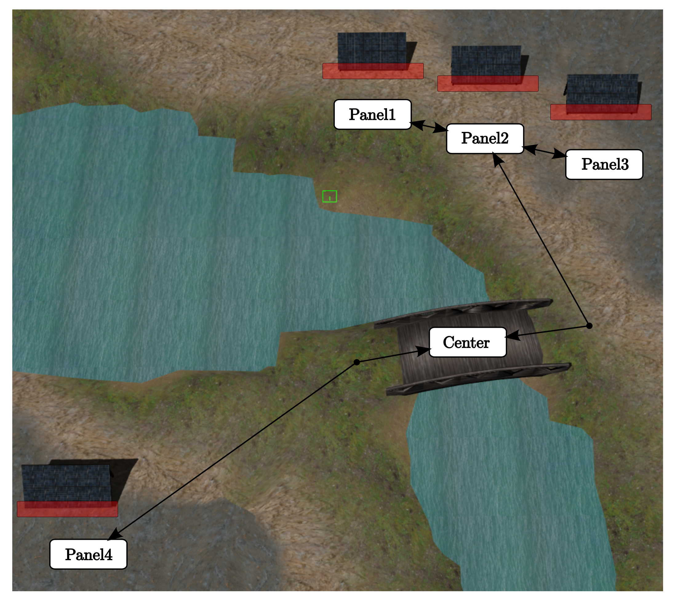
In this subsection, we address a multi-robot inspection application with the proposed toolbox. The problem consists in a solar farm with four photovoltaic panels that require regular inspection. The inspection is carried by two small unmanned ground vehicles (UGVs) that have limited battery autonomy. A larger UGV that carries bigger batteries acts as a mobile charger and can recharge one small UGV at a time. The goal is to maximize the number of times all four solar panels are inspected.
Figure 12 shows the solar farm world implemented in Gazebo. Overlapped on this world, the topological map the robots use to navigate is depicted. The terrain is uneven and it introduces wheel slippage that increases the uncertainty during navigation. There is also uncertainty associated with the time it takes to inspect each solar panel and with battery charging and discharging.
The simulation was implemented in ROS and it was tested in ROS Noetic and Melodic versions. The small UGVs and the large UGV used were Clearpath’s Jackal UGVs and Warthog UGV, respectively. The localization was obtained from an extended Kalman filter algorithm that uses fused GPS, IMU and odometry sensor data. To navigate we used the move-base package without any modifications. The Gazebo world can be found in [28], the Jackal’s packages are in [29] and the Warthog packages are in [30]. These repositories were built from Clearpath’s source code and adapted to enable multiple robots operating simultaneously. A video with the system executing can be visualized here: (youtube.com/watch?v=SzpZBFmJZn8, accessed on 1 November 2021).
To capture this application as a GSPNR model we used the toolbox design method that builds the model from a given topological map and action models. The final GSPNR is one single connected model but is the result of merging two different models. One model that captures the small UGVs and another that captures the large UGV actions and dynamics. The tokens in these models never flow from one to the other, ensuring distinction between the two types of robots. The small UGV model captures navigation, inspection and recharge actions. The large UGV model captures navigation and recharge actions since this type of robot only acts as a mobile charger and is not able to inspect. The actions that require cooperation such as the battery recharge are the only parts where both models meet. This is detailed bellow when present the recharging model. Having different models for each robot type enables heterogeneous multi-robot modeling, while maintaining the representation of each robot as a token. With this representation the state space grows with multichoose multichoose , where and are the places and tokens of the small UGV and the large UGV, respectively. Still, it grows slower than having a GSPNR model per robot, given that each type has more than one robot. This approach is scalable for more than two types of robots, by applying the same method of building separate models and connecting them through the cooperative actions.
The goal is not to decide when is the best time to recharge, but where should the robots be, and in which order should they inspect the solar panels, such that, when they need to recharge they can do it as efficiently as possible. For this reason, we discretized the battery of the small UGVs in two levels: high and low. On the lower level the small UGVs cannot perform any action besides recharging. So if when one small UGV discharges it cannot move, and has to wait until the Warthog decides to move to that location.
Figure 13 depicts the small UGV action models. Figure 13 (Left) shows the navigation action model instantiated between panel 1 and panel 2. The immediate transition GoPanel1-Panel2HighBat captures the action selection and the timed transition ArrivedPanel1-Panel2HighBat models the traverse time uncertainty. The weights of the immediate transitions DischargedPanel1-Panel2HighToHigh and DischargedPanel1-Panel2HighToLow create the probability distribution that captures the probability of the battery level dropping to low or not. This is possible due to the extension introduced in Section 3.2. The navigation model is replicated for every edge of the topological map.
Figure 13 (Center) shows the inspection action model in panel 1. This model is similar to the navigation model with the difference that the action selection transition InspectPanel1HighBat has an extra input place (r.InspectionRequiredPanel1) and an extra output place (r.AlreadyInspected). The tokens in these places do not represent robots, instead act as memory places that limit to one the amount of times a solar panel can be inspected each round. There is one r.InspectionRequiredPanel place per panel, while the r.AlreadyInspected is unique. So when a panel is inspected a token is consumed from the r.InspectionRequiredPanel place and created on the r.AlreadyInspected. When all panels are inspected the r.AlreadyInspected output transition fires and these tokens flow back to the r.InspectionRequiredPanel places. This ensures that the system only inspects the same panel again when all the other panels have been inspected. The toolbox interprets the characters r. before the place name, and takes that place as a special place, treating the tokens inside as system resources and not as robots. This has no consequence in the model synthesis, but has an impact in the task plan execution. During execution, these tokens are not mapped into robots and do not interact with any action server. These work as another state factor, creating memory that enables the distinction between states before and after the inspection action is executed. The inspection model is replicated for all topological map nodes, except the center node.
Figure 13 (Right) shows the recharging model. This GSPNR acts as interface between the small UGVs and the large UGV models since recharging is an action that requires synchronized cooperation between both robots. This synchronization is ensured since the transition ChargePanel1 is only enabled when at least one small UGV with low battery is on the same location as the large UGV.
To capture multiple battery levels for each individual robot we propose a novel approach that is depicted in Figure 14. The GSNPR model that captures the small UGVs’ navigation and inspection actions is replicated as many times as there are battery levels. Then, all the discharging transitions that lead to a lower battery level are connected to the level immediately bellow. Thus, the tokens that represent robots with the battery fully charged are flowing in the part of the GSPNR that corresponds to level 1. Once one of these robots loses some percentage of battery charge, the discharging transitions fire, and the token moves to level 2. When the robot is fully discharged and is nearby a large UGV it is able to select the recharge action and that moves the token back to level 1. This approach is more efficient in terms of state space size when compared to building a GSPNR per robot and model individually its battery level.
The goal is to inspect all panels as quickly as possible and as many times as possible. Therefore, the defined reward function yields a reward of for every solar panel inspection transition fired. It also gives a place reward of per unit of time for every small UGV that has low battery. This discourages the system from keeping robots with low battery for long periods of time. We used a discount factor of 0.99 and a convergence error of 0.01.
The GSPNR model parameters were estimated by running every action once and using the action duration to compute the timed transitions rates. We obtained the optimal policy using the toolbox policy synthesis module, that we shall call GSPNR policy. We then executed and compared the policy obtained with the toolbox against a policy synthesized from a marked ordinary Petri net model. We also compared it against two baselines: a random policy and an handcrafted policy. The random policy consists of randomly choosing an action every time the system has to make a decision. The handcrafted policy was carefully designed and follows a greedy policy. As a result, the small UGVs choose to inspect the closest available panel, while the large UGV stays stationary in the last node visited until a small UGV discharges. When this occurs the large UGV moves to the closest discharged robot and initiates the charging procedure. The main difference between the MOPN model and the GSPNR is that the former does not capture time uncertainty since it only has immediate transitions. So the MOPN model is identical to the GSPNR model described above, but the timed transitions were replaced by immediate transitions. The immediate transitions, that replace the timed transitions, have weights assigned that are proportional to the time that it takes to execute that action. So if a particular action takes less time, then the probability of the corresponding transition firing is higher. Moreover, the place rewards disappear in this model since there is no notion of continuous time. So we only provide a positive transition reward, that is given when an inspection action is selected. Each policy was executed in the simulated Gazebo environment for 8 runs of 1 h each.
The number of solar panels inspected over time is depicted in Figure 15. The handcrafted policy is substantially better than the random policy showing that it is highly efficient. Nevertheless, both policies obtained from the GSPNR and the MOPN models outperform the handcrafted policy. This shows that formal methods are able to produce more efficient behaviors than carefully engineered policies. Longer runs suggest that as time increases the GSPNR policy diverges further from the handcrafted policy.
The designed MOPN model does not capture time uncertainty, but it is able to model uncertainty in the outcomes of actions. As a result, the MOPN is able to distinguish between longer actions and shorter actions as the latter occur more often. The GSPNR captures time uncertainty as an exponential distribution, that, in some cases, does not correspond to the action duration true distribution. Nevertheless, the GSPNR policy outperforms the MOPN policy providing evidence that taking action duration uncertainty into account can improve the quality of the yielded policy. The standard deviation of the GSPNR policy is larger than of the MOPN policy. This occurs since the GSPNR model forces the system to always select an action, unlike in the MOPN. The consequence is that, for example the large UGV moves around significantly more, and crosses in front of the small UGVs more often. Thus the path planning algorithm introduces an higher variability in the time it takes to move between locations. For this reason, around second 1750 the MOPN policy has more solar panels inspected, on average, than the GSPNR policy. Finally, the MOPN model state space grows as fast as the GSPNR model, existing no difference in the time it takes to synthesize the optimal policy.
Figure 16 shows the charging periods of the multi-robot system for the GSPNR policy and the handcrafted policy. A thorough analysis of the plots and the execution video shows that one of the reasons why the GSPNR policy performs better is how it handles recharges. The GSPNR policy tries to synchronize the discharge of the robots in the same location. Thus, usually, it is able to recharge both robots in the same place one after the other. Furthermore, when the two robots are simultaneously discharged the mobile charger gives preference to the one closer to a solar panel that requires inspection. As a result, the first robot to be recharged can more quickly resume the inspection round while the other robot is recharged.
4. Conclusions
Building models is usually a cumbersome task and is prone to design errors. Having tools that are easy to use and simplify the design process is important when trying to mitigate these errors. Furthermore, visually intuitive models, formal guarantees, and qualitative and quantitative analysis also helps in this task. Plus, being able to sample from the model and simulate the policy behavior allows us to detect possible modeling errors or undesired policy behaviors.
This work tackles these issues and introduces a toolbox that provides straightforward access to modeling, planning and execution methods for multi-robot systems. To do that, the toolbox leverages state-of-the-art approaches such as GSPNRs for multi-robot systems and implements dynamic programming techniques to obtain optimal control policies. This not only allows us to model, in a compact form, multi-robot problems but also to produce control policies that reason over uncertainty in the action duration while optimizing team-level objectives. Furthermore, it introduces novel GSPNR building methods as an effort to simplify complex model design. Finally, the task plans that result from applying the obtained policy to the model built, can be directly executed in ROS in a lightweight tool that provides robust and fluid execution.
The toolbox was used to solve a solar farm inspection application. The resulting task plan was executed in Gazebo, and was compared against a handcrafted approach and an MOPN approach that does not consider time uncertainty. The results show that our approach outperforms the others, providing evidence that accounting for time uncertainty yields more efficient behaviors.
Nevertheless, as with all model based approaches, it suffers from rapid state space growth. Despite translating into a linear growth in model memory, it prevents the use of exact solution methods as these scale quadractically with the number of states. Thus, for future work, we intend to investigate and incorporate into this tool alternative policy synthesis methods. We intend to explore the synthesis of sub-optimal policies and with that be able to scale for larger teams.
Author Contributions
Conceptualization, C.A.; methodology, C.A.; software, C.A. and A.M.; investigation, C.A. and A.M.; writing—original draft preparation, C.A.; writing—review and editing, A.M., P.U.L. and J.A.; supervision, P.U.L.; funding acquisition, C.A. and P.U.L. All authors have read and agreed to the published version of the manuscript.
Funding
This work was supported by the Portuguese Foundation for Science and Technology (FCT) under the grant SFRH/BD/135014/2017, by the INTERREG ATLANTIC programme under the subsidy contract EAPA_986/2018 and through the RoboCup Federation and Mathworks research projects for 2021.
Data Availability Statement
The developed toolbox can be found in https://github.com/cazevedo/multi-robot-gspnr-toolbox accessed on 16 December 2021. The Gazebo world can be found in https://github.com/cazevedo/cpr_gazebo/tree/ros-noetic/cpr_inspection_gazebo accessed on 16 December 2021. The multi-robot packages can be found in https://github.com/amdpaula/multi_jackal and in https://github.com/amdpaula/multi_warthog accessed on 16 December 2021.
Conflicts of Interest
The authors declare no conflict of interest. The funders had no role in the design of the study; in the collection, analyses, or interpretation of data; in the writing of the manuscript, or in the decision to publish the results.
Abbreviations
The following abbreviations are used in this manuscript:
| GSPN | Generalized Stochastic Petri Net |
| GSPNR | Generalized Stochastic Petri Net with Rewards |
| MOPN | Marked Ordinary Petri Net |
| MDP | Markov Decision Process |
| MMDP | Multi-Agent Markov Decision Process |
| ROS | Robot Operating System |
| UGV | Unmanned Ground Vehicle |
| CPU | Central Processing Unit |
References
- Ohradzansky, M.T.; Rush, E.R.; Riley, D.G.; Mills, A.B.; Ahmad, S.; McGuire, S.; Biggie, H.; Harlow, K.; Miles, M.J.; Frew, E.W.; et al. Multi-Agent Autonomy: Advancements and Challenges in Subterranean Exploration. arXiv 2021, arXiv:2110.04390. [Google Scholar]
- Soetens, R.; van de Molengraft, R.; Cunha, B. Robocup msl-history, accomplishments, current status and challenges ahead. In Robot Soccer World Cup; Springer: Cham, Switzerland, 2014; pp. 624–635. [Google Scholar]
- Visser, U.; Burkhard, H.D. RoboCup: 10 years of achievements and future challenges. AI Mag. 2007, 28, 115. [Google Scholar]
- Benkrid, A.; Benallegue, A.; Achour, N. Multi-robot coordination for energy-efficient exploration. J. Control Autom. Electr. Syst. 2019, 30, 911–920. [Google Scholar] [CrossRef]
- Mannucci, A.; Pallottino, L.; Pecora, F. On Provably Safe and Live Multirobot Coordination with Online Goal Posting. IEEE Trans. Robot. 2021, 37, 1973–1991. [Google Scholar] [CrossRef]
- Rouček, T.; Pecka, M.; Čížek, P.; Petříček, T.; Bayer, J.; Šalanskỳ, V.; Heřt, D.; Petrlík, M.; Báča, T.; Spurnỳ, V.; et al. Darpa subterranean challenge: Multi-robotic exploration of underground environments. In Proceedings of the International Conference on Modelling and Simulation for Autonomous Systesm, Palermo, Italy, 29–31 October 2019; pp. 274–290. [Google Scholar] [CrossRef]
- Pecora, F.; Andreasson, H.; Mansouri, M.; Petkov, V. A Loosely-Coupled Approach for Multi-Robot Coordination, Motion Planning and Control. In Proceedings of the International Conference on Automated Planning and Scheduling (ICAPS), Delft, The Netherlands, 24–29 June 2018. [Google Scholar]
- Schwab, D. Robot Deep Reinforcement Learning: Tensor State-Action Spaces and Auxiliary Task Learning with Multiple State Representations. Ph.D. Thesis, Carnegie Mellon University, Pittsburgh, PA, USA, 2020. [Google Scholar]
- Vasic, M.; Billard, A. Safety issues in human-robot interactions. In Proceedings of the IEEE International Conference on Robotics and Automation, Karlsruhe, Germany, 6–10 May 2013; pp. 197–204. [Google Scholar]
- Burdick, J.W.; du Toit, N.; Howard, A.; Looman, C.; Ma, J.; Murray, R.M.; Wongpiromsarn, T. Sensing, Navigation and Reasoning Technologies for the DARPA Urban Challenge; Technical Report; California Inst of Technology Pasadena JET Propulsion Lab: Pasadena, CA, USA, 2007. [Google Scholar]
- Coogan, S.; Arcak, M.; Belta, C. Finite state abstraction and formal methods for traffic flow networks. In Proceedings of the 2016 American Control Conference (ACC), Boston, MA, USA, 6–8 July 2016; pp. 864–879. [Google Scholar]
- Fraser, D.; Giaquinta, R.; Hoffmann, R.; Ireland, M.; Miller, A.; Norman, G. Collaborative Models for Autonomous Systems Controller Synthesis. Form. Asp. Comput. 2020, 32, 157–186. [Google Scholar] [CrossRef] [Green Version]
- Kwiatkowska, M.; Norman, G.; Parker, D. PRISM: Probabilistic symbolic model checker. In Proceedings of the International Conference on Modelling Techniques and Tools for Computer Performance Evaluation, London, UK, 14–17 April 2002; Springer: Berlin/Heidelberg, Germany, 2002; pp. 200–204. [Google Scholar]
- Hensel, C.; Junges, S.; Katoen, J.P.; Quatmann, T.; Volk, M. The probabilistic model checker Storm. arXiv 2020, arXiv:2002.07080. [Google Scholar] [CrossRef]
- Dingle, N.J.; Knottenbelt, W.J.; Suto, T. PIPE2: A tool for the performance evaluation of generalised stochastic Petri Nets. ACM Sigmetrics Perform. Eval. Rev. 2009, 36, 34–39. [Google Scholar] [CrossRef]
- Chiola, G.; Franceschinis, G.; Gaeta, R.; Ribaudo, M. GreatSPN 1.7: Graphical editor and analyzer for timed and stochastic Petri nets. Perform. Eval. 1995, 24, 47–68. [Google Scholar] [CrossRef]
- Bohren, J.; Cousins, S. The smach high-level executive [ros news]. IEEE Robot. Autom. Mag. 2010, 17, 18–20. [Google Scholar] [CrossRef]
- Ziparo, V.A.; Iocchi, L.; Lima, P.U.; Nardi, D.; Palamara, P.F. Petri Net Plans—A framework for collaboration and coordination in multi-robot systems. Auton. Agents Multi-Agent Syst. 2011, 23, 344–383. [Google Scholar] [CrossRef]
- Cashmore, M.; Fox, M.; Long, D.; Magazzeni, D.; Ridder, B.; Carrera, A.; Palomeras, N.; Hurtos, N.; Carreras, M. Rosplan: Planning in the robot operating system. In Proceedings of the International Conference on Automated Planning and Scheduling, Jerusalem, Israel, 7–11 June 2015; Volume 25. [Google Scholar]
- Azevedo, C.; Lacerda, B.; Hawes, N.; Lima, P. Long-Run Multi-Robot Planning under Uncertain Action Durations for Persistent Tasks. In Proceedings of the IEEE/RSJ International Conference on Intelligent Robots and Systems (IROS), Las Vegas, NV, USA, 24 October–24 January 2020. [Google Scholar]
- Boutilier, C. Sequential optimality and coordination in multiagent systems. In Proceedings of the International Joint Conference on Artificial Intelligence (IJCAI), Stockholm, Sweden, 31 July–6 August 1999; Volume 99, pp. 478–485. [Google Scholar]
- Balbo, G. Introduction to generalized stochastic Petri nets. In Proceedings of the International School on Formal Methods for the Design of Computer, Communication and Software Systems, Bertinoro, Italy, 8 May–2 June 2007. [Google Scholar]
- Azevedo, C.; Lacerda, B.; Hawes, N.; Lima, P. Long-Run Multi-Robot Planning With Uncertain Task Durations. In Proceedings of the 19th International Conference on Autonomous Agents and MultiAgent Systems, Auckland, New Zealand, 9–13 May 2020; pp. 1750–1752. [Google Scholar]
- Azevedo, C.; Paula, A.; Lima, P.; Avendano, J. Multi-Robot GSPNR Toolbox. 2021. Available online: http://github.com/cazevedo/multi-robot-gspnr-toolbox (accessed on 1 November 2021).
- Akharware, N.; Miee, M. Pipe2: Platform Independent Petri Net Editor; The Pennsylvania State University: University Park, PA, USA, 2005. [Google Scholar]
- Puterman, M.L. Markov Decision Processes: Discrete Stochastic Dynamic Programming; John Wiley & Sons Inc.: Hoboken, NJ, USA, 2014. [Google Scholar]
- Costelha, H.; Lima, P. Robot task plan representation by Petri nets; Modelling, identification, analysis and execution. Auton. Robot. 2012, 33, 337–360. [Google Scholar] [CrossRef]
- Azevedo, C.; Paula, A.; Lima, P.; Avendano, J. Solar Farm Gazebo World. 2021. Available online: https://github.com/cazevedo/cpr_gazebo/tree/ros-noetic/cpr_inspection_gazebo (accessed on 1 November 2021).
- Azevedo, C.; Paula, A.; Lima, P.; Avendano, J. Multi-Jackal ROS Packages. 2021. Available online: https://github.com/amdpaula/multi_jackal (accessed on 1 November 2021).
- Azevedo, C.; Paula, A.; Lima, P.; Avendano, J. Multi-Warthog ROS Packages. Available online: https://github.com/amdpaula/multi_warthog (accessed on 1 November 2021).
Figure 1.
(Left) Topological map with 3 locations; (Right) GSPNR model of two robots navigating the topological map depicted on the left.
Figure 1.
(Left) Topological map with 3 locations; (Right) GSPNR model of two robots navigating the topological map depicted on the left.

Figure 2.
MATLAB® GSPNR Toolbox architecture interfaced with peripheral toolboxes.

Figure 3.
(Left) Navigation action model; (Center) Vacuuming action model; (Right) Mopping action model.
Figure 3.
(Left) Navigation action model; (Center) Vacuuming action model; (Right) Mopping action model.

Figure 4.
GSPNR obtained from the composition of the models in Figure 3 and the topological map in Figure 1 (Left).

Figure 5.
Diagram summarizing the policy synthesis algorithm.

Figure 6.
(Left) GSPNR example; (Right) Equivalent MDP obtained from the GSPNR on the left.

Figure 7.
Execution manager algorithm flowchart.

Figure 8.
(Left) Time required to generate the GSPNR model as the number of locations grows, where n represents the number of locations; (Right) Time required to generate the GSPNR model as the number of robots grows.
Figure 8.
(Left) Time required to generate the GSPNR model as the number of locations grows, where n represents the number of locations; (Right) Time required to generate the GSPNR model as the number of robots grows.

Figure 9.
(Left) State space size as a function of the number of locations; (Right) State space size as a function of the number of robots, where p represents the number of places and r the number of tokens in the GSPNR model.
Figure 9.
(Left) State space size as a function of the number of locations; (Right) State space size as a function of the number of robots, where p represents the number of places and r the number of tokens in the GSPNR model.

Figure 10.
(Left) MDP conversion time and value iteration convergence time as the state space grows; (Right) Average time that each iteration takes when performing value iteration, where s represents the number of states.
Figure 10.
(Left) MDP conversion time and value iteration convergence time as the state space grows; (Right) Average time that each iteration takes when performing value iteration, where s represents the number of states.

Figure 11.
(Top Left) Execution module CPU usage as the number of locations increases; (Top Right) Execution module memory usage as the number of locations increases; (Bottom Left) Execution module CPU usage as the number of robots increases; (Bottom Right) Execution module memory usage as the number of robots increases.

Figure 12.
Solar farm Gazebo world with the topological map overlapped. The red rectangles represent the area that must be covered to ensure a reliable solar panel inspection.
Figure 12.
Solar farm Gazebo world with the topological map overlapped. The red rectangles represent the area that must be covered to ensure a reliable solar panel inspection.

Figure 13.
(Left) Navigation model with battery discharging transitions; (Center) Inspection model with battery discharging transitions and number of inspections counter; (Right) Recharging model.
Figure 13.
(Left) Navigation model with battery discharging transitions; (Center) Inspection model with battery discharging transitions and number of inspections counter; (Right) Recharging model.

Figure 14.
Solar farm full GSPNR model with N battery levels and recharge action. Blue color—inspection model; yellow color—navigation model; red color—discharging model; green color—recharging model.
Figure 14.
Solar farm full GSPNR model with N battery levels and recharge action. Blue color—inspection model; yellow color—navigation model; red color—discharging model; green color—recharging model.

Figure 15.
Number of panels inspected by each policy as time progresses. The solid line represents the average value over 8 runs and the shaded area the standard deviation.
Figure 15.
Number of panels inspected by each policy as time progresses. The solid line represents the average value over 8 runs and the shaded area the standard deviation.

Figure 16.
System recharging periods (shaded areas) overlapped with the number of inspections (solid line). Blue color—GSPNR policy; Green color—handcrafted policy.
Figure 16.
System recharging periods (shaded areas) overlapped with the number of inspections (solid line). Blue color—GSPNR policy; Green color—handcrafted policy.

Publisher’s Note: MDPI stays neutral with regard to jurisdictional claims in published maps and institutional affiliations. |
© 2021 by the authors. Licensee MDPI, Basel, Switzerland. This article is an open access article distributed under the terms and conditions of the Creative Commons Attribution (CC BY) license (https://creativecommons.org/licenses/by/4.0/).
Share and Cite
MDPI and ACS Style
Azevedo, C.; Matos, A.; Lima, P.U.; Avendaño, J. Petri Net Toolbox for Multi-Robot Planning under Uncertainty. Appl. Sci. 2021, 11, 12087. https://0-doi-org.brum.beds.ac.uk/10.3390/app112412087
AMA Style
Azevedo C, Matos A, Lima PU, Avendaño J. Petri Net Toolbox for Multi-Robot Planning under Uncertainty. Applied Sciences. 2021; 11(24):12087. https://0-doi-org.brum.beds.ac.uk/10.3390/app112412087
Chicago/Turabian StyleAzevedo, Carlos, António Matos, Pedro U. Lima, and Jose Avendaño. 2021. "Petri Net Toolbox for Multi-Robot Planning under Uncertainty" Applied Sciences 11, no. 24: 12087. https://0-doi-org.brum.beds.ac.uk/10.3390/app112412087
Note that from the first issue of 2016, this journal uses article numbers instead of page numbers. See further details here.