
An Intelligent Diagnosis Method for Machine Fault Based on Federated Learning


1
Key Laboratory of Nondestructive Testing Ministry of Education, Nanchang Hangkong University, Nanchang 330063, China
2
School of Mechanical Engineering, Guangxi University, Nanning 530004, China
3
Laboratory of Science and Technology on Integrated Logistics Support, National University of Defense Technology, Changsha 410073, China
4
Shaanxi Key Laboratory of Mine Electromechanical Equipment Intelligent Monitoring, Xi’an University of Science and Technology, Xi’an 710054, China
*
Author to whom correspondence should be addressed.
Appl. Sci. 2021, 11(24), 12117; https://0-doi-org.brum.beds.ac.uk/10.3390/app112412117
Submission received: 4 November 2021
/
Revised: 8 December 2021
/
Accepted: 14 December 2021
/
Published: 20 December 2021
(This article belongs to the Special Issue Soft Computing Application to Engineering Design)
Abstract
:In engineering, the fault data unevenly distribute and difficultly share, which causes that the existing fault diagnosis methods cannot recognize the newly added fault types. An intelligent diagnosis method for machine fault is proposed based on federated learning. Firstly, the local fault diagnosis models diagnosing the existing fault data and the newly added fault data are established by deep convolutional neural network. Then, the weight parameters of local models are fused into global model parameters by federated learning. Finally, the global model parameters are transmitted to each local model. Therefore, each local model update into a global shared model which can recognize the newly added fault types. The proposed method is verified by bearing data. Compared with the traditional model, which can only diagnose the existing fault data but cannot recognize newly added fault types, the federated fault diagnosis model fusing weight parameters can diagnose newly added faults without exchanging the data, and the accuracy is 100%. The proposed method provides an effective method to solve the poor sharing of fault data and poor generalization of fault diagnosis model for mechanical equipment.
1. Introduction
In the era of big data, the amount of data obtained by sensors is very large, and the data types are diverse. The fault diagnosis methods based on deep learning make it possible for mechanical big data processing. However, the reliable fault diagnosis model based on deep learning depends on abundant fault data. In engineering, different enterprises own the different types of fault data and the data from different enterprises is private and hardly shared, so the established fault model cannot recognize the newly added fault types. Therefore, it is of great significance how to establish a shared fault diagnosis model without exchanging data so that the model can recognize newly added fault types.
At present, the mechanical fault diagnosis method based on deep learning has been widely studied. For example, in Ref. [1], a deep belief network was used to diagnose the health of aero-engines. In Ref. [2], the fault diagnosis in bearings and planetary gearboxes is successfully completed by a deep neural network, which overcomes the deficiency in traditional signal processing methods, i.e., traditional signal processing excessively relying on expert knowledge. In Ref. [3], a new hierarchical network based on deep belief network was proposed to diagnose the fault damage degree of rolling bearings. In Ref. [4], a deep convolutional neural network was used to monitor gearboxes to extract features adaptively. Compared with features extracted from time domain and frequency domain, those extracted by deep convolutional neural network are better. In Ref. [5], a deep autoencoder has been successfully applied into the fault diagnosis of bearings and gears. In Ref. [6], in order to better adapt to the one-dimensionality of the bearing and gear vibration signals, one-dimensional deep convolutional neural network was used for fault diagnosis. In Ref. [7], a normalized deep convolutional neural network was proposed to solve the imbalance of fault data. In Ref. [8], the bearing signal was compressed and collected by compressed sensing and classified by deep learning. In Ref. [9], a deep convolutional neural network model was used for end-to-end fault diagnosis of noisy signals. In Ref. [10], a novel deep capsule network with random delta rules was proposed to solve the problems of load variation and noise in bearing vibration signals. In Ref. [11], a fault diagnosis method of sparse autoencoders was proposed to recognize different coupling faults of bearings. In Ref. [12], the combination of deep learning and transfer learning was used for fault diagnose of rotating machinery. In Ref. [13], a deep residual neural network was proposed for fault diagnosis of rolling bearing; the proposed method can prevent gradient disappearance and gradient explosion. In Ref. [14], deep transfer learning was applied to diagnose the fault of rolling bearing under variable conditions, and the recognition rate is improved by 2–8%. In Ref. [15], a deep convolutional neural network was used to recognize the fault types based on the fusion data collected by the horizontal and vertical sensors mounted in the gearbox. In Ref. [16], the sparse denoising autoencoder and transfer learning was combined to diagnose bearing faults. In Ref. [17], a transfer model of fault diagnosis was established by deep residual neural network. The proposed model can transfer laboratory data to actual engineering data and has a high recognition rate. In Ref. [18], a multi-source transfer learning network was proposed to solve sample imbalance of mechanical fault by getting together and transferring the diagnosis knowledge modules of multiple machines.
In summary, the existing mechanical fault diagnosis methods can be roughly divided into two categories, which are shown in Figure 1.
- (1)
- In Figure 1a, the multi-fault diagnosis models are used to recognize the different fault types.
- (2)
- In Figure 1b, the data of different fault types are fused to construct a sample set, which can be used to establish a diagnosis model which can recognize different fault types.
However, none of these recognition methods of fault diagnosis consider the problem of the data privacy and sharing, resulting in the established fault diagnosis model not being able to recognize the newly added fault types. Therefore, a shared fault diagnosis model is expected to be proposed to recognize the newly added fault types without exchanging fault data.
Federated Learning (FL) [19,20], as a distributed machine learning algorithm, is mainly used to train data distributed on a large number of client nodes to obtain a high-quality model. That is, the local model can be trained by FL on the client node without exchanging data samples, and these local model parameters are updated at a certain frequency, so that the local model is updated to the global model. Theodora et al. [21] applied FL into electronic health medical prediction. For a large number of medical data distributed in individuals or other hospitals, they fused the patient information by FL to predict the probability of a patient being hospitalized due to heart disease. Andrew et al. [22] applied FL into the input prediction of the mobile phone keyboard and predicted the next input word by establishing a shared model based on the data of multiple mobile phones. Kang et al. [23] introduced the reputation metric into FL to improve the reliability of federated learning models in mobile networks. Süzen et al. [24] applied FL into health care so that medical institutions could diagnose new types of diseases without exchanging data. Therefore, the idea of FL provides the possibility for a fault diagnosis model with a shared mechanism.
Based on the distinguished advantages of FL, FL was introduced into mechanical fault diagnosis. An intelligent diagnosis method based on FL was proposed for mechanical faults. The main works of this paper are as follows.
- (1)
- The proposed method can effectively recognize new fault types and improve the generalization ability of fault diagnosis model.
- (2)
- A local fault diagnosis model is established for different types of fault data and is fused into a federated fault diagnosis model by the proposed method, which solves the hardly shared problem in different types of fault data.
- (3)
- The process of federated fault diagnosis model is explained by visualizing the weight distribution.
The rest of this paper is organized as follows. In Section 2. the theoretical basis and implementation steps of a fault diagnosis model based on federated learning are proposed. In Section 3. the effectiveness of the proposed method is verified by two bearing cases, and the proposed method is compared with the traditional fault diagnosis method. The value conclusions are drawn in Section 4.
2. The Shared Fault Diagnosis Model Based on Federated Learning
2.1. Proposed Methodology
The architecture of shared fault diagnosis model based on FL is shown in Figure 2. Firstly, a local fault diagnosis model should be established. Because deep learning with good self-feature extraction and classification capabilities has been applied widely in fault diagnosis, the local fault diagnosis models are constructed based on deep convolutional neural networks. In general, a deep convolutional neural network model is constituted by an input layer, a convolution layer, a pooling layer, a fully connected layer, and an output layer [25]. The convolution layer mines the hidden features of the input data by the convolution kernel and expresses it in high-dimensional form. The pooling layer can reduce the output dimensionality of the convolution layer and extract local features, so as to accelerate the convergence and ensure the invariance of space and structure. The fully connected layer and the output layer are used to classify. The structure of the deep convolution neural network used in this paper is shown in Figure 2. The individual local fault diagnosis models established based on the structure can recognize the trained fault types, that is, the models find the classification hyperplane that can recognize the faults, as shown ①, ② and ③ in Figure 2. From ④ in Figure 2, no matter which hyperplane cannot accurately and effectively classify all faults. However, the fault diagnosis model based on FL finds a classification hyperplane suitable for recognizing the faults with different types, as shown ⑤ in Figure 2. The reason is that the model based on FL fuses the weight parameters of each local fault diagnosis model into global weight. Then, the global weight parameters are returned to the local model to update as a global shared federated fault diagnosis model.
The specific steps of establishing the federated fault diagnosis model are as follows.
Step 1. The local fault diagnosis models are established. A fault data set Fk (k = 1, 2, 3, ···, K) is constructed from the vibration signals of the monitored key components, and the set is divided into the training set and the testing set according to a certain proportion. K local models for K fault data sets are established respectively.
Step 2. Initialize the federated learning model parameters and train the model. The model parameters are initialized, such as model weight w, maximum number of iterations N, total number of local fault diagnosis models K, score of nodes used in local fault diagnosis model C, batch size B, and learning rate η.
During each iteration t (t = 1, 2, 3, ···, N), m (m = max(C × K, 1)) nodes are selected from the above K local fault diagnosis models, and a random training sample set (k = 1, 2, 3, ···, m) is constructed. At the same time, local parameters Model Update (k, ) are updated by training the local models.
During the training process, the batch size is b, so, i (i = 1, 2, ..., length()/b) calculations are performed in each iteration. Therefore, the input is = (1 + b × (i−1):b × i).
In the forward propagation process of training, the input (l = 1, 2, …, L, L is the number of convolution layer) are convolved with the convolution kernel when it passes the l-th convolution layer. Then, the output is obtained as:
where * is the convolution operation, biasl is the bias, and f () is the activation function.
The output (p = 1, 2, …, P, P is the number of pooling layer) of the p-th convolution layer is calculated by the maximum pooling in the l-th pooling layer, i.e.,:
where maxpooling () is the maximum pooling calculation and is the output of the pooling layer.
In the fully connected layer, the output of the last pooling layer is flattened as:
The output of the fully connected layer xfc is obtained by calculating the flattened xfl in the fully connected layer, i.e.,:
Finally, the output of the fully connected layer is classified in the output layer. In the fully connected layer, the softmax is commonly used as the classifier, namely:
where is the predicted output of the model.
By calculating the loss function J (, b), the error between the actual label input y and the predicted output is minimized to improve the accuracy of the model, i.e.,:
where is the set of convolution weights and fully connected layer weights wfc and loss (, b) is the loss function of each batch.
After calculating the loss function in the forward propagation of the local diagnosis model, the weight parameters are derived and updated through back propagation, namely:
where is the weight vector of the local diagnosis model k in each global iteration t and := represents the update operation.
After the local weights are updated, the local weights are merged into the global weights, namely:
where is the local weight of the k-th local fault diagnosis model, nk is the number of training samples in the local fault diagnosis model, n is the total number of samples, and wt+1 is the global weight parameter.
The global weight wt+1 is returned to the local fault diagnosis model, and the next iteration is performed until the maximum number of iterations N is reached.
Step 3. If the loss value of the model trained in Step 2 does not converge, Step 2 will be repeated. If the loss value after training drops and converges to 0, the model is successful. Finally, the generalization ability of the model is verified through the testing set. If the generalization ability is good, the model will be applied to diagnose fault. If not, Step 1 will be restarted. The local models after training are all global models.
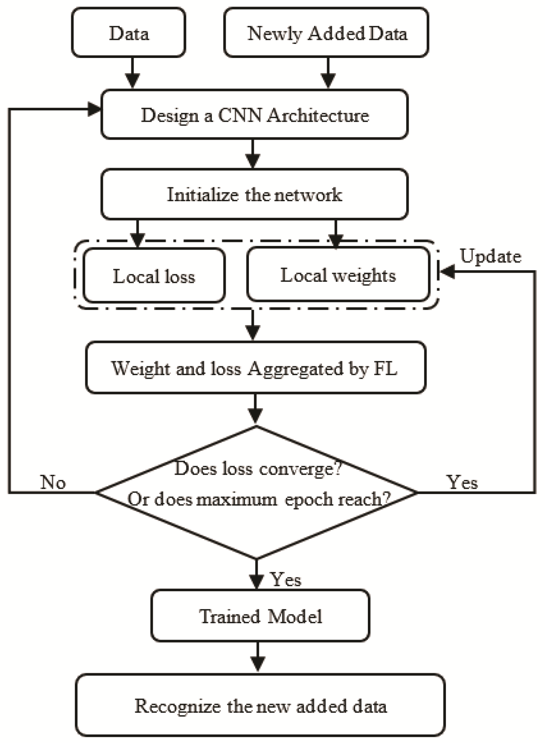
The flowchart of proposed fault diagnosis model is presented in Figure 3.
2.2. Parameters Selection
The values of parameters and hyperparameters are obtained through many experiments and literature. According to reference [26,27], the parameters of convolution layer and pool layer in a convolution neural network is designed, as shown in Table 1. The design of hyperparameters in the proposed method is shown in Table 2. The score of the client node is usually set to C = 1, so that all local parameters can be updated in each iteration. In order to train all client samples as a single minimum batch, the batch size B = ∞ is usually set in each iteration [19].
2.3. Performance Evaluation
To evaluate the performance of the proposed method, the accuracy can be calculated by Equation (10) [28].
In Equation (10), the TP, FN, TN and FP represent the number of true positives, false negatives, true negatives and false positives, respectively. Moreover, the loss, as in Equation (6), plays an important role in adjusting the overfitting or underfitting. Further, to observe the class separability, the feature space of the output of convolution layer is visualized by t-distribution stochastic neighbor embedding (t-SNE) [29].
3. Case Study
In this section, two cases, containing the Machinery Fault Database datasets [30] and Case Western Reserve University datasets [31], are used to verify the effectiveness of the built FL model. Two experiments were performed based on the TensorFlow Federated of FL framework in CentOS 7.0 platform. The basic information of the platform is as follows. The CPU is [email protected] GHz, the Python version is 3.7.4, the TensorFlow version is 2.2.0, and the TensorFlow Federated version is 0.14.0.
3.1. Case 1: Bearing Fault Data of Machinery Fault Database
In this section, the bearing fault data from the Machinery Fault Database [30] are used. The data are obtained on the quasi-balance vibration trainer in Spectra Quest’s mechanical failure simulator. During the operation of the test rig with rotating frequency of 30 Hz and no load, the acceleration data of the bearing between the rotor and the motor are collected at the sampling frequency of 51.2 kHz, and the sampling time is 5 s. The sample data are collected under four working conditions, i.e., normal, inner fault, outer fault, and ball fault. There are 400 samples for each bearing working condition. The samples are divided into training set and testing set according to the ratio of 9:1.
For the four working conditions of the bearing, four local fault diagnosis models based on deep convolution neural network are constructed according to the parameters in Table 1 and Table 2, i.e., the models Mn, Mb, Mi, and Mo. Then, the four models are fused by FL. After the fusing, the local models are update as a global model. Figure 4 shows the loss curve and accuracy curve after the training and testing. The loss of the testing set gradually converges to 0, and almost overlaps with that of the training set in the entire model. The accuracy of the training set and the testing set all reach 100%. So, the federated fault diagnosis model can recognize all fault types. In order to better explain the federated fault diagnosis model, the weights of each convolution layer are visualized, as shown in Figure 5. Comparing the distribution of initialized weights in Figure 5a, the distribution of weights after training changes in Figure 5b. The result reflects the change process of the model parameters before and after the training.
The feature extraction ability of the federated fault diagnosis model can be shown by the hidden features of the convolution layer. However, since the output of the convolution layer is a high-dimensional vector, it is not easy to display. Therefore, it is necessary to reduce the dimension of output of the convolution layer. Here, the non-linear dimensionality reduction algorithm t-SNE is employed. After dimension reduction, the scatter diagrams of hidden features from each convolution layer are shown in Figure 6. From Figure 6, it can be seen that the features of faults with different types are gradually separated, and the features of the same fault types are gradually gathered. So, the federated fault diagnosis model can recognize different conditions of the bearing.
In order to demonstrate the advantages of the proposed model, the comparison with the local fault diagnosis model is conducted. Firstly, the four local models Mn, Mb, Mi, and Mo are used to analyze the single working condition corresponding to the model, and the results are shown in Figure 7. From Figure 7, the loss curves of the training set and testing set of each model all decrease to zero, and the accuracy curves all reach 100%. At the same time, the curves of the training set and the testing set almost overlap, which indicates that the overfitting or underfitting has not arisen in the model. Therefore, the local fault diagnosis models are well trained and used to recognize the single fault type.
Then, we constructed a hybrid testing set to test the local fault diagnosis model and the federated fault diagnosis model. The hybrid set is composed of the data under four working conditions according to the ratio of 1:1:1:1. The testing result of the models is as shown in Table 3. By observing Table 3, it can be found that the loss is 0 and the accuracy is 100% when the local fault diagnosis models are tested by their corresponding fault types. However, when the local fault diagnosis models are tested by the hybrid testing set, the loss increases and the accuracy decreases. Each local model can only recognize its corresponding fault type, so the accuracy is only 25%. In other words, the local models cannot recognize the other three fault types. Therefore, it is difficult to diagnose other faults with a single local fault diagnosis model, which makes it impossible to effectively monitor the bearing. When the federated fault diagnosis model Mfed is tested by the hybrid testing set, the loss is 0 and the accuracy is 100%. It can be seen that the federated fault diagnosis model can recognize a variety of fault types.
Finally, the weight distribution of these models is analyzed. Figure 8 shows the weight distribution of local fault diagnosis models. From Figure 7, the weight distribution of the same layer in the four local models is very different, because the four local models are trained, respectively, for the different fault types. When tested by the data for other fault types, the local models are naturally unable to recognize.
By comparing the weights distribution in Figure 5 and Figure 8, it is found that the weight obtained by the Mfed is a balanced value of the weight of each local models. So, the model with this weight can diagnose a variety of faults. Through the above analysis, the proposed federated fault diagnosis model has a good effect on recognizing different fault types of bearings, and the accuracy is 100%.
3.2. Case 2: Bearing Fault Data of Case Western Reserve University
In Case 1, the effectiveness of the FL model has been verified. In Case 2, the effectiveness of the FL model in fusing local fault diagnosis models that recognize multiple fault types is explored. Here, the data of SKF6205 bearing at the driving end are used, which is from Case Western Reserve University [31]. The data were collected under a load of 1.0 kN and a speed of 1772 r/min. The bearing data under ten kinds of working conditions are used, i.e., no fault, 0.007-inch ball fault, 0.007 inch inner fault, 0.007 inch outer fault, 0.014 inch ball fault, 0.014 inch inner fault, 0.014 inch outer fault, 0.021 inch ball fault, 0.021 inch inner fault, and 0.021 inch outer fault. Each working condition has 400 samples, and there are a total of 4000 samples. This is assuming that there are four models, which still adopt the deep convolution neural network shown in Figure 2. The four models are trained according to the different conditions. Therefore, different models have different fault diagnosis capabilities, as shown in Table 4.
Then, the weight of the four models is fused and optimized through FL, so that each model has the same fault diagnosis capability. The results of training and testing are shown in Figure 9. Figure 9a shows the loss curves of the training set and the testing set. It can be seen that the loss gradually converges and tends to 0 as the iteration, which reflects that the model finds the optimal value and does not fall into an overfitting state. Figure 9b shows the accuracy curves of the training set and the testing set, and the accuracy is 100%. The two curves almost overlap, which reflects that there is no overfitting and underfitting in the model. So, the generalization ability of the model is very good. The weight distribution of each convolution layer in the federated fault diagnosis model is shown in Figure 10. By comparing Figure 10a with Figure 10b, the weight changes, which reflects the training process of the model.
In order to further observe the effectiveness of the federated fault diagnosis model, the t-SNE algorithm is also used to reduce the dimensionality of the output of each convolution layer in the model. The features scatter diagram performed is shown in Figure 11. From Figure 11a, it can be seen that the features of the data with different conditions are aliasing, i.e., there is a strong correlation among them. Only the features of the 0.007-inch ball fault and 0.021-inch ball fault are roughly clustered, and other fault features are in a chaotic state. Especially, the features of normal conditions are submerged in those of fault conditions. Figure 11b depicts the fault features extracted by the second convolution layer in the model. After calculating by two convolution layers, the features begin to be clustered, and the features of normal conditions begin to appear. The features of the 0.007-inch ball fault, 0.014-inch outer fault, and 0.021-inch ball fault are more obvious. Figure 11c shows the features extracted by the third convolution layer in the model. It can be seen that the features are clustered and separated clearly. Only the features of the 0.021-inch outer fault and the 0.007-inch inner fault overlap. Figure 11d shows the features extracted by the fourth convolution layer in the model; the features of the ten conditions are clearly separated and the various fault features are completely gathered, which intuitively reflects the effectiveness of the model.
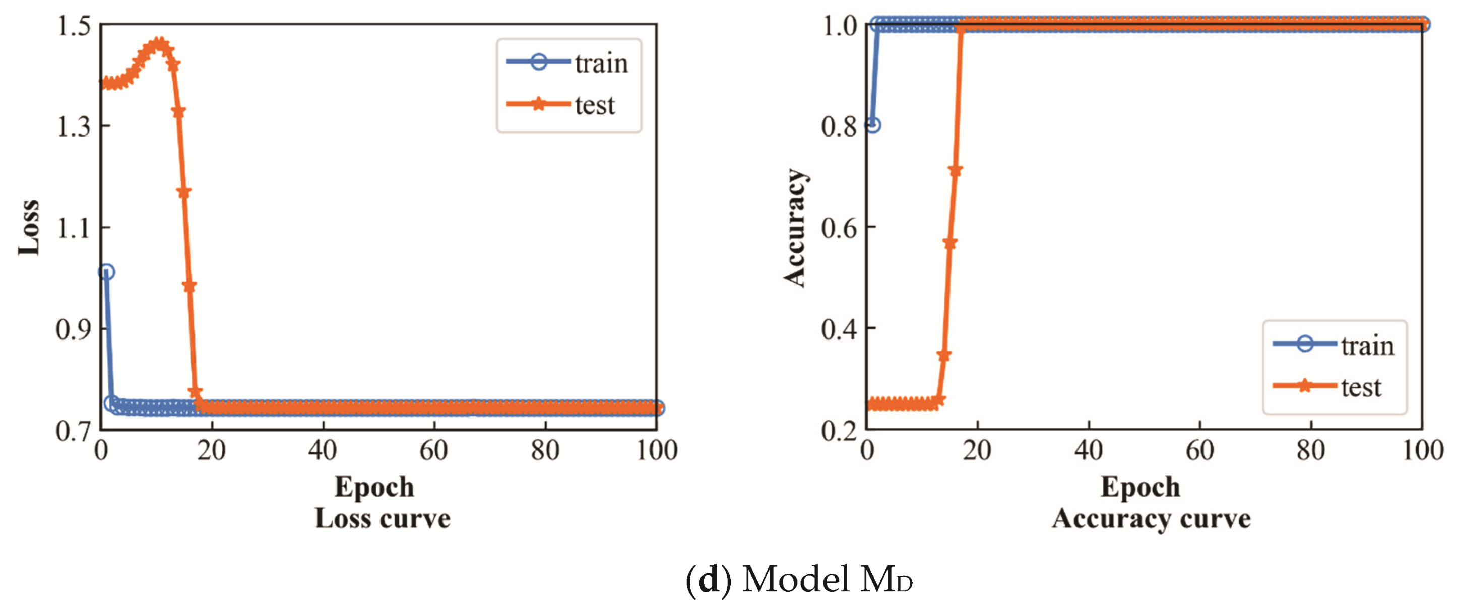
In order to demonstrate the advantages of the proposed model, the comparison with the local fault diagnosis model MA, MB, MC, and MD is conducted. The results of these local models are shown in Figure 12. From Figure 12, the loss curve of the training set and testing set of each model decreases steadily and gradually converges. The accuracy curves of the training set and the testing set gradually rise to almost 100%, and the accuracy curves almost overlap, so overfitting and underfitting does not happen in the model. Therefore, the local fault diagnosis model is better trained and can recognize the type of fault which has been trained by itself.
Next, a hybrid testing set containing ten working conditions is used to test the local fault diagnosis models and the federated fault diagnosis model. The data ratios of the ten working conditions are the same. Table 5 shows the test results. It is found that the loss is close to 0 and the accuracy is 100% when the local models are tested by their corresponding fault types. However, the loss becomes larger, and the accuracy decreases, when the local models are tested by the hybrid testing set. Therefore, the local models can only diagnose the trained type of fault and cannot recognize the newly added fault type. When the federated fault diagnosis model Mfed is tested by the hybrid testing set, the loss is 0 and the accuracy is 100%. This indicates that the model Mfed can diagnose all fault types.
Then, the weight of the local models is visualized to analyze. Figure 13 shows the weight distribution of each convolution layer of the local fault diagnosis model. Due to the local models with the different fault diagnosis capability, the weight distribution of the same layer in each local model is very different. Therefore, the local models naturally cannot make a diagnosis when tested by the data for other fault types.
From the comparison of Figure 10 and Figure 13, it is found that the weight of the federated fault diagnosis model is a balanced value of the weight of the local models, so that the proposed model can diagnose all fault types. Through the above analysis, the established federated fault diagnosis model shows good results in recognizing different types of bearings, and the accuracy is 100%.
4. Conclusions
An intelligent diagnosis model for mechanical fault based on federated learning was proposed and verified by two bearing cases. The proposed method solves the problems that the fault data share difficultly, and the newly added fault types cannot be recognized. The following conclusions are drawn. The federated fault diagnosis model established based on the proposed method can recognize the newly added fault type, because the weight parameters of local model are fused and updated during the training. The proposed model achieves the effect of data sharing by fusing the models with different fault recognition capabilities to recognize the different fault types. By the weight distribution of the model, it is found that the weight of the proposed model is a balanced value of the weights of local fault diagnosis models. Compared with the traditional fault diagnosis model, the proposed model can recognize the multiple fault types with an accuracy of 100%.
Author Contributions
Z.L. (Zhinong Li) was in charge of the whole trial, Z.L. (Zedong Li) and Y.L. wrote the manuscript, J.T. was assisted with resources, and Q.M. and X.Z. validated. All authors have read and agreed to the published version of the manuscript.
Funding
This work was supported by the grant from the National Natural Science Foundation of China (Grant No. 52075236), the Laboratory of Science and Technology on Integrated Logistics Support, National University of Defense Technology (Grant No. 6142003190210), key projects of the Natural Science Foundation of Jiangxi Province (Grant No. 20212ACB202005), and the Shaanxi Key Laboratory of Mine Electromechanical Equipment Intelligent Monitoring (Grant No. SKL-MEEIM201901).
Institutional Review Board Statement
Not applicable.
Informed Consent Statement
Not applicable.
Data Availability Statement
Data sharing is not applicable to this article.
Conflicts of Interest
The authors declare no conflict of interest.
References
- Tamilselvan, P.; Wang, P.F. Failure diagnosis using deep belief learning based health state classification. Reliab. Eng. Syst. Saf. 2013, 115, 124–135. [Google Scholar] [CrossRef]
- Jia, F.; Lei, Y.G.; Lin, J.; Zhou, X.; Lu, N. Deep neural networks: A promising tool for fault characteristic mining and intelligent diagnosis of rotating machinery with massive data. Mech. Syst. Signal Process. 2016, 72–73, 303–315. [Google Scholar] [CrossRef]
- Gan, M.; Wang, C.; Zhu, C.A. Construction of hierarchical diagnosis network based on deep learning and its application in the fault pattern recognition of rolling element bearings. Mech. Syst. Signal Process. 2016, 72–73, 92–104. [Google Scholar] [CrossRef]
- Jing, L.Y.; Zhao, M.; Li, P.; Xu, X.Q. A convolutional neural network based feature learning and fault diagnosis method for the condition monitoring of gearbox. Measuremen 2017, 111, 1–10. [Google Scholar] [CrossRef]
- Shao, H.D.; Jiang, H.K.; Zhao, H.W.; Wang, F.A. A novel deep autoencoder feature learning method for rotating machinery fault diagnosis. Mech. Syst. Signal Process. 2017, 95, 187–204. [Google Scholar] [CrossRef]
- Zhou, Q.C.; Liu, X.C.; Zhao, J.; Shen, H.H.; Xiong, X.L. Fault diagnosis for rotating machinery based on 1D depth convolutional neural network. J. Vib. Shock 2018, 37, 31–37. [Google Scholar]
- Jia, F.; Lei, Y.G.; Lu, N.; Xing, S.B. Deep normalized convolutional neural network for imbalanced fault classification of machinery and its understanding via visualization. Mech. Syst. Signal Process. 2018, 110, 349–367. [Google Scholar] [CrossRef]
- Wen, J.T.; Yan, C.H.; Sun, J.D.; Qiao, Y.L. Bearing fault diagnosis method based on compressed acquisition and deep learning. Chin. J. Sci. Instrum. 2018, 39, 171–179. [Google Scholar]
- Zhang, W.; Li, C.H.; Peng, G.L.; Chen, Y.H.; Zhang, Z.J. A deep convolutional neural network with new training methods for bearing fault diagnosis under noisy environment and different working load. Mech. Syst. Signal Process 2018, 108, 33–47. [Google Scholar] [CrossRef]
- Chen, T.Y.; Wang, Z.H.; Yang, X.; Jiang, K. A deep capsule neural network with stochastic delta rule for bearing fault diagnosis on raw vibration signals. Measurement 2019, 148, 106857. [Google Scholar] [CrossRef]
- Yang, J.; Xie, G.; Yang, Y.X.; Li, X.; Mu, L.X.; Takahashi, S.; Mochizuki, H. An improved deep network for intelligent diagnosis of machinery faults with similar features. IEEE Trans. Electr. Electron. Eng. 2019, 14, 1851–1864. [Google Scholar] [CrossRef]
- Qian, W.W.; Li, S.M.; Jiang, X.X. Deep transfer network for rotating machine fault analysis. Pattern Recognit. 2019, 96, 106993. [Google Scholar] [CrossRef]
- Zhang, W.; Li, X.; Ding, Q. Deep residual learning-based fault diagnosis method for rotating machinery. ISA Trans. 2019, 95, 295–305. [Google Scholar] [CrossRef] [PubMed]
- Che, C.C.; Wang, H.W.; Fu, Q.; Ni, X.M. Deep transfer learning for rolling bearing fault diagnosis under variable operating conditions. Adv. Mech. Eng. 2019, 11, 1687814019897212. [Google Scholar] [CrossRef] [Green Version]
- Chen, H.P.; Hu, N.Q.; Cheng, Z.; Zhang, L.; Zhang, Y. A deep convolutional neural network based fusion method of two-direction vibration signal data for health state identification of planetary gearboxes. Measurement 2019, 146, 268–278. [Google Scholar] [CrossRef]
- Sun, M.D.; Wang, H.; Liu, P.; Huang, S.D.; Fan, P. A sparse stacked denoising autoencoder with optimized transfer learning applied to the fault diagnosis of rolling bearings. Measurement 2019, 146, 305–314. [Google Scholar] [CrossRef]
- Yang, B.; Lei, Y.G.; Jia, F.; Xing, S.B. An intelligent fault diagnosis approach based on transfer learning from laboratory bearings to locomotive bearings. Mech. Syst. Signal Process. 2019, 122, 692–706. [Google Scholar] [CrossRef]
- Yang, B.; Xu, S.C.; Lei, Y.G.; Lee, C.G.; Stewart, E.; Roberts, C. Multi-source transfer learning network to complement knowledge for intelligent diagnosis of machines with unseen faults. Mech. Syst. Signal Process. 2022, 162, 108095. [Google Scholar] [CrossRef]
- McMahan, H.B.; Moore, E.; Ramage, D.; Hampson, S.; Arcas, B.A. Communication-Efficient Learning of Deep Networks from Decentralized Data. In Proceedings of the Machine Learning Research; Singh, A., Zhu, J., Eds.; PMLR: Fort Lauderdale, FL, USA, 2017; Volume 54, pp. 1273–1282. [Google Scholar]
- Liu, Y.; Liu, Y.T.; Liu, Z.J.; Liang, Y.X.; Meng, C.S.; Zhang, J.B.; Zheng, Y. Federated Forest. IEEE Trans. Big Data 2020. [Google Scholar] [CrossRef]
- Theodora, S.B.; Chen, R.D.; Theofanie, M.; Olshevsky, A.; Paschalidis, L.C.; Shi, W. Federated learning of predictive models from federated electronic health records. Int. J. Med Inform. 2018, 112, 59–67. [Google Scholar]
- Andrew, H.; Kanishka, R.; Rajiv, M.; Rajiv, M.; Francoise, B.; Sean, A.; Hubert, E.; Chloe, K.; Daniel, R. Federated learning for mobile keyboard prediction. arXiv 2019, arXiv:1811.03604. [Google Scholar]
- Kang, J.W.; Xiong, Z.H.; Niyato, D.; Zou, Y.Z.; Zhang, Y.; Guizani, M. Reliable federated learning for mobile networks. IEEE Wirel. Commun. 2020, 27, 72–80. [Google Scholar] [CrossRef] [Green Version]
- Süzen, A.A.; Simek, M.A. A novel approach to machine learning application to protection privacy data in healthcare: Federated learning. Namik Kemal Tip Derg. 2020, 8, 22–30. [Google Scholar]
- Yu, S.Q.; Jia, S.; Yan, C. Convolutional neural networks for hyperspectral image classification. Neurocomputing 2017, 219, 88–89. [Google Scholar] [CrossRef]
- Zhang, W.; Peng, G.L.; Li, C.H.; Chen, Y.H.; Zhang, Z.J. A new deep learning model for fault diagnosis with good Anti-noise and Domain Adaption Ability on Raw Vibration Signals. Sensors 2017, 17, 425. [Google Scholar] [CrossRef]
- Szegedy, C.; Vanhoucke, V.; Loffe, S.; Shlens, J.; Wojna, Z. Rethinking the Inception Architecture for computer vision. In Computer Vision and Pattern Recognition (CVPR); Springer Science & Business Media: Las Vegas, NV, USA, 2016; Volume 1, pp. 2818–2826. [Google Scholar]
- Luque, A.; Carrasco, A.; Matin, A.; de las Heras, A. The impact of class imbalance in classification performance metrics based on the binary confusion matrix. Pattern Recognit. 2019, 91, 216–231. [Google Scholar] [CrossRef]
- Laurens, V.D.M.; Hinton, G. Visualizing data using t-SNE. J. Mach. Learn. Res. 2008, 9, 2579–2605. [Google Scholar]
- Marins, M.A.; Ribeiro, F.M.L.; Netto, S.L.; Silva, E.A.B. Improved similarity-based modeling for the classification of rotating-machine failures. J. Frankl. Inst. 2018, 355, 1913–1930. [Google Scholar] [CrossRef]
- Smith, W.A.; Randall, R.B. Rolling element bearing diagnosis using the Case Western reserve university data: A benchmark study. Mech. Syst. Signal Process. 2015, 64–65, 100–131. [Google Scholar] [CrossRef]
Figure 1.
Existing fault diagnosis methods.

Figure 2.
Architecture of federated fault diagnosis model.

Figure 3.
Flowchart of the proposed model.

Figure 4.
Loss and accuracy curve of federated fault diagnosis model.

Figure 5.
Weight distribution of the federated fault diagnosis model.

Figure 6.
Features scatter diagram based on the proposed model.

Figure 7.
Loss and accuracy curve of local fault diagnosis model.


Figure 8.
Weight distribution of the local fault diagnosis models.


Figure 9.
Loss curve and accuracy curve of federated fault diagnosis model.

Figure 10.
Weight distribution of the federated fault diagnosis model.

Figure 11.
Features scatter diagram based on the proposed model.

Figure 12.
Loss curve and accuracy curves of local fault diagnosis model.


Figure 13.
The weight distribution of the local fault diagnosis models.


Table 1.
Parameters of deep convolution neural network.
| Layers | Size | Stride | Output | Activation Function |
|---|---|---|---|---|
| Input | 1 × 1024 | |||
| Convolution layer 1 (C1) | 8 × 1 × 5 | 1 × 1 | 8 × 1 × 1020 | ReLU |
| Convolution layer 2 (C2) | 8 × 1 × 5 | 1 × 1 | 8 × 1 × 1016 | ReLU |
| Pooling layer 1 (P1) | 1 × 2 | 1 × 2 | 8 × 1 × 508 | |
| Convolution layer 3 (C3) | 16 × 1 × 3 | 1 × 1 | 16 × 1 × 506 | ReLU |
| Convolution layer 4 (C4) | 16 × 1 × 3 | 1 × 1 | 16 × 1 × 504 | ReLU |
| Pooling layer 2 (P2) | 1 × 2 | 1 × 2 | 16 × 1 × 252 | |
| Flatten (F1) | 4032 | |||
| Fully connection (F2) | 1000 | ReLU | ||
| Output | 10 | Softmax |
Table 2.
Hyperparameters of Federated Learning.
| Hyperparameters | Value |
|---|---|
| Iteration N | 100 |
| Score of nodes C | 1 |
| Batch size B | ∞ |
| Batch size of client b | 32 |
| Learning rate η | 0.0001 |
| Dropout | 0.4 |
Table 3.
Comparison between local fault diagnosis model and federated fault diagnosis model.
| Model | The Testing Set Contains One Fault Type | The Hybrid Testing Set Contains Four Faults Types | ||
|---|---|---|---|---|
| Loss | Accuracy | Loss | Accuracy | |
| Mn | 0.0 | 100% | 12.0766 | 25% |
| Mb | 0.0 | 100% | 10.0846 | 25% |
| Mi | 0.0 | 100% | 12.0883 | 25% |
| Mo | 0.0 | 100% | 11.7205 | 25% |
| Mfed | 0.0 | 100% | ||
Table 4.
Models with different fault diagnosis capability.
| Model | Fault Diagnosis Capability |
|---|---|
| Model A | Nine types of fault expect 0.021 inch Outer fault |
| Model B | Normal and 0.007 inch Inner fault, Outer fault, and Ball fault |
| Model C | Normal and 0.014 inch Inner fault, Outer fault, and Ball fault |
| Model D | Normal and 0.021 inch Inner fault, Outer fault, and Ball fault |
Table 5.
Comparison of loss and accuracy of the two models.
| Model | The Testing Set Contains Trained Fault Types | The Testing Set Contains Ten Types of Faults | ||
|---|---|---|---|---|
| Loss | Accuracy | Loss | Accuracy | |
| MA | 1.3720 | 97.37% | 10.9775 | 85.67% |
| MB | 0.7437 | 100% | 54.3214 | 40% |
| MC | 0.7437 | 100% | 52.8715 | 40% |
| MD | 0.7437 | 100% | 64.1308 | 40% |
| Mfed | 0.0 | 100% | ||
Publisher’s Note: MDPI stays neutral with regard to jurisdictional claims in published maps and institutional affiliations. |
© 2021 by the authors. Licensee MDPI, Basel, Switzerland. This article is an open access article distributed under the terms and conditions of the Creative Commons Attribution (CC BY) license (https://creativecommons.org/licenses/by/4.0/).
Share and Cite
MDPI and ACS Style
Li, Z.; Li, Z.; Li, Y.; Tao, J.; Mao, Q.; Zhang, X. An Intelligent Diagnosis Method for Machine Fault Based on Federated Learning. Appl. Sci. 2021, 11, 12117. https://0-doi-org.brum.beds.ac.uk/10.3390/app112412117
AMA Style
Li Z, Li Z, Li Y, Tao J, Mao Q, Zhang X. An Intelligent Diagnosis Method for Machine Fault Based on Federated Learning. Applied Sciences. 2021; 11(24):12117. https://0-doi-org.brum.beds.ac.uk/10.3390/app112412117
Chicago/Turabian StyleLi, Zhinong, Zedong Li, Yunlong Li, Junyong Tao, Qinghua Mao, and Xuhui Zhang. 2021. "An Intelligent Diagnosis Method for Machine Fault Based on Federated Learning" Applied Sciences 11, no. 24: 12117. https://0-doi-org.brum.beds.ac.uk/10.3390/app112412117
Note that from the first issue of 2016, this journal uses article numbers instead of page numbers. See further details here.