Automatic Generation of Aerial Orthoimages Using Sentinel-2 Satellite Imagery with a Context-Based Deep Learning Approach

Abstract

Aerial images are an outstanding option for observing terrain with their high-resolution (HR) capability. The high operational cost of aerial images makes it difficult to acquire periodic observation of the region of interest. Satellite imagery is an alternative for the problem, but low-resolution is an obstacle. In this study, we proposed a context-based approach to simulate the 10 m resolution of Sentinel-2 imagery to produce 2.5 and 5.0 m prediction images using the aerial orthoimage acquired over the same period. The proposed model was compared with an enhanced deep super-resolution network (EDSR), which has excellent performance among the existing super-resolution (SR) deep learning algorithms, using the peak signal-to-noise ratio (PSNR), structural similarity index measure (SSIM), and root-mean-squared error (RMSE). Our context-based ResU-Net outperformed the EDSR in all three metrics. The inclusion of the 60 m resolution of Sentinel-2 imagery performs better through fine-tuning. When 60 m images were included, RMSE decreased, and PSNR and SSIM increased. The result also validated that the denser the neural network, the higher the quality. Moreover, the accuracy is much higher when both denser feature dimensions and the 60 m images were used.

1. Introduction

Aerial imagery has been widely used for monitoring the surrounding environment due to its long history. Orthoimages created from aerial images can provide high-quality geospatial information taken at lower altitudes than satellite images. Continuously monitoring a rapidly changing environment requires reducing the observation period for a site. However, the tradeoff between spatial resolution and ground coverage prevents aerial images from covering a wide area. The role of aerial imagery has been gradually replaced by satellite imagery with its wide area coverage and regular repeat pass capabilities. Moreover, satellites equipped with multispectral sensors have enabled multiple applications such as resource management, urban research, facility mapping, and disaster monitoring.

The resolution of most of the current satellite images is still lower than that of aerial images. The price of commercially available high-resolution (HR) satellites has frequently hindered many researchers’ progress in their projects. In most countries, including Korea, HR aerial orthoimages are provided to the public for free [1]. Furthermore, in the United States and the European Union, low- and medium-resolution satellite images are provided free of charge to users around the world. Research is needed to increase the resolution of mid- and low-resolution satellite images using freely available HR aerial images.

In the field of remote sensing, a visible improvement of image resolution primarily implies pan-sharpening. This method improves the resolution of low-resolution multispectral images using an HR panchromatic image. There are two typical approaches, one using Intensity-Hue-Saturation (IHS) information [2] and one using principal component analysis (PCA) [3]. The primary concern for pan-sharpening is that it is applicable only when an HR panchromatic image is available. Consequently, the resolution of the pan-sharpened image cannot be higher than that of the input panchromatic image. With the recent development of deep learning techniques, studies to produce images with higher resolution than the input image have been conducted. Several studies using deep learning techniques have been published in the remote sensing community. Related studies can be largely divided into two usage categories: multiple sensors from one platform and multiple sensors from multiple platforms [4,5,6,7,8,9,10].

Improving the resolution of multispectral sensors from one (same) platform is usually performed by merging lower and higher multispectral images. Gargiulo et al. [5] enhanced a 20 m shortwave infrared (SWIR) image acquired by Sentinel-2 into a 10 m SWIR image. Similar to the pan-sharpening approach, the four-channel 10 m visible and NIR resolution images of Sentinel-2 were regarded as panchromatic. A shallow convolutional neural network (CNN) was constructed to improve the resolution of the SWIR image. The limitation of this study is that only the resolution of an SWIR image can be improved. Lanaras et al. [6] presented research results that can address this limitation. By constructing deep and dense neural network models, DSen2 and VDSen2, they improved the 20 m resolution of three red-edge and three SWIR images, two 60 m resolution images of water vapor, and 60 m SWIR mages of Sentinel-2 images into 10 m. They asserted that the model could be extended and improved from 20 m and 60 m to a 10 m resolution. However, the first category cannot produce images with higher resolution than the maximum resolution provided by the platform.

Another category is improving the resolution of multispectral sensors from multiple (different) platforms. Few studies have improved 30 m Landsat-8 satellite images to 10 m using Sentinel-2 images. Shao et al. [7] proposed the extended super-resolution convolutional neural network (ESRCNN) by blending Landsat-8 and Sentinel-2 data. They demonstrated the effectiveness of the deep learning-based fusion method for improving the resolution of Landsat-8 imagery. In their study, a performance comparison was performed using area-to-point regression kriging rather than other deep learning-based algorithms. Pouliot et al. [9] tested shallow and deep CNNs and confirmed that the deep CNN performed the same or better than the shallow CNN. The suggested algorithm demonstrated high-performance, but computational complexity and memory requirements could be problematic because the model is trained for each band.

After analyzing the previous studies, we found three common points. The first is that the use of deep neural networks is superior [6,8,9]. Tai et al. [8] analyzed the performance of each neural network by constructing shallow, deep, and very deep networks. They confirmed that the deeper the neural network, the higher the performance. Second, most neural networks have residual blocks and skip connections [6,8,10,11]. Consequently, the vanishing gradient problem can be alleviated, and the learning speed improved, even though the neural network is deeper. Third, the size of the input image inside the neural network is maintained until the last stage of the output, in contrast to neural networks for object detection and segmentation. Accordingly, the enlargement function to create the HR is only located in the final stage of neural networks using upsampling convolution layers or pixel shuffle algorithms [11]. Galar et al. [10] applied an enhanced deep super-resolution network (EDSR) to produce a 5 m resolution RapidEye RGB image with a 10 m resolution Sentinel-2 RGB image. They confirmed superior performance among super-resolution (SR) neural networks [11,12].

Studies so far have used neural networks of increasing resolution between satellite images. In this study, we propose a context-based ResU-Net to increase the resolution of Sentinel-2 imagery using 2.5 and 5.0 m downsampled aerial orthoimage acquired during the same period. For completing the tasks, the aerial orthoimages were first simulated by reconstructing a residual U-Net, which has advantages not only in constructing a deep and dense neural network but also in identifying adjacent contexts and the position of objects. As a result of the experiments, we found that our neural network can express the aerial orthoimages’ features and contexts well.

Training datasets were newly generated by using Sentinel-2 and aerial orthoimage. Sentinel-2 images, providing 10 m, 20 m, and 60 m resolution of multispectral bands, were utilized in this research. Sentinel-2 has the highest resolution and shortest revisit date among free satellite images. Since the advantage of obtaining many repeat pass images is a factor that can satisfy the objectives of this study, it was selected as input data. SR research is key to securing a high-resolution ground truth (GT), and aerial orthoimages are one of the most reliable and high-quality data. Therefore, aerial orthoimages with a similar acquisition date were utilized as the GT. Two types of aerial orthoimages were produced, 2.5 m and 5.0 m, as ground truth data downsampled from the original aerial orthoimagery. The data were used for testing two-times magnification (5.0 m based on 10 m) and challenged four-time magnification (2.5 m based on 10 m).

We tested the effect of using the lowest resolution 60 m image on the model and analyzed the model’s influence when the feature dimensions are changed. In addition, the quality of our approach was investigated through the peak signal-to-noise ratio (PSNR), structural similarity index measure (SSIM), and root-mean-squared error (RMSE), a common approach in many SR studies.

Finally, we found that our model’s performance in most metrics turned out to be better than that of EDSR. We also identified that incorporating 60 m resolution with 10 m resolution Sentinel-2 images outperforms the combination 10 m and 20 m resolution images. In addition, we confirmed that the denser feature dimensions have better performance. In particular, it could be a useful reference for related research as it predicts well even narrow roads that are difficult to identify with low-resolution satellite images.

2. Materials and Methods

2.1. Training Datasets Generation and Site Selection

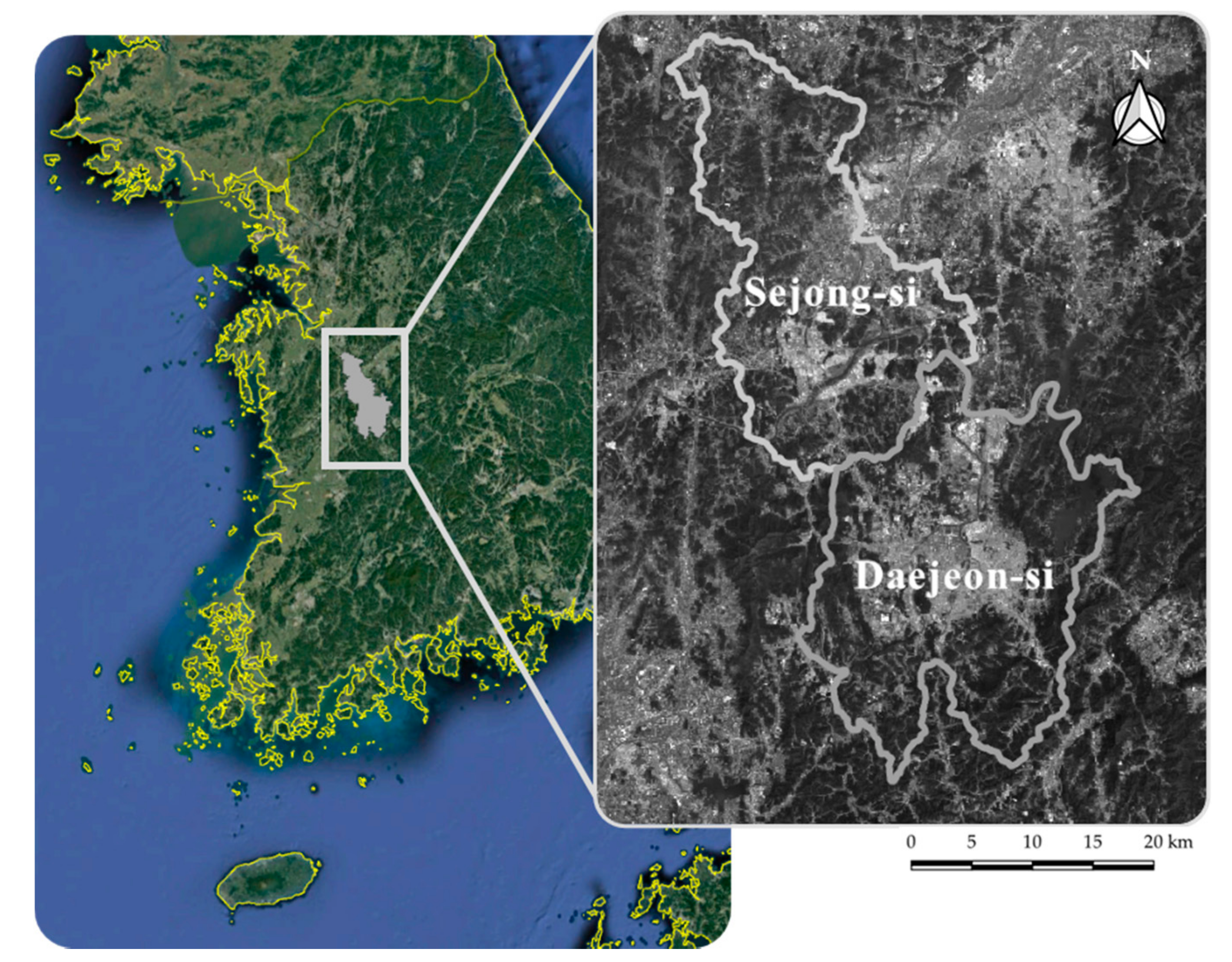
2.1.1. Study Area

Daejeon City, located in the central part of the Korean peninsula, was selected as the study area. The city has an area of approximately 539 km² and is a transportation hub connecting the southern and northern regions. As depicted in Figure 1, most of the areas illustrate urban landscapes, where large and small buildings are clustered. Rice paddies/fields and mountainous areas are distributed in minimal areas. Middle areas, primarily covered with many complex environments such as urban buildings and roads, are the areas where the SR approach is challenging to apply.

Sejong City, Korea’s administrative capital, is being developed into a city since 2012. The area of Sejong City is approximately 465 km², and most of the regions are still mountains and rice fields. However, due to construction, the impermeable layer is increasing rapidly every year. Daejeon City was selected to produce training datasets, and Sejong City was selected as a test site to analyze the generalization capabilities. Even if training samples and test samples are not overlapped, spatial autocorrelation within the same area cannot be avoided. Therefore, it was necessary to select an independent region with different characteristics.

2.1.2. Aerial Orthoimages

Aerial orthoimages were acquired in 2018, distributed free of charge under the leadership of the Korean government’s aerial image acquisition and map production policy. Due to national security reasons, only 51 cm resolution images are provided to the public [1], and internally up to a 25 cm resolution is produced and used. We meticulously inspected the acquisition date of aerial images through the government orthoimage production manual and identified that aerial images were acquired over approximately one month, 21 April, 29 April, 5 May, and 26 May 2018, to cover the entire study area. The 51 cm orthoimages using the aerial triangulation method were provided through the government website. The final orthoimages downloaded are depicted in Figure 2.

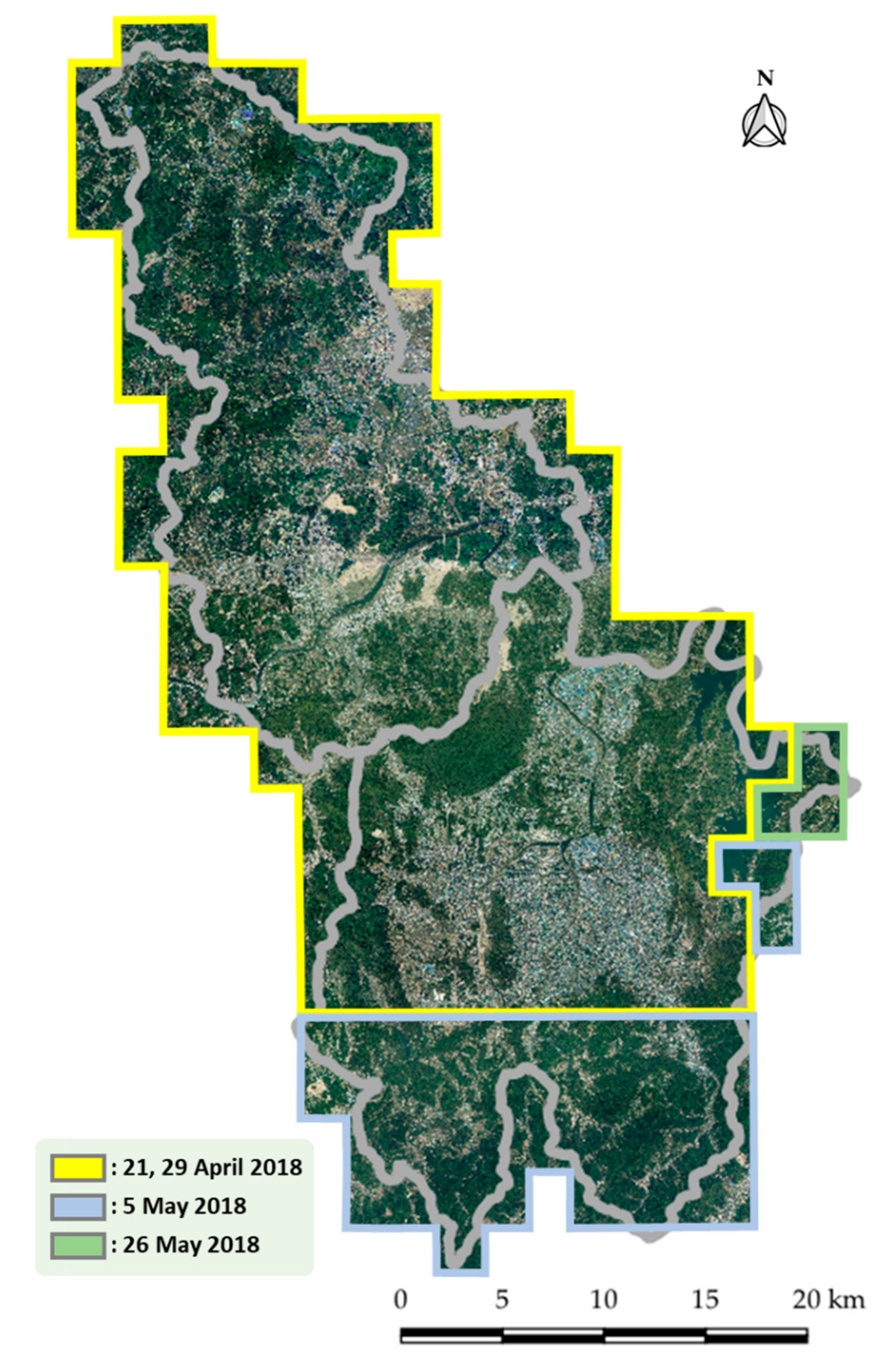
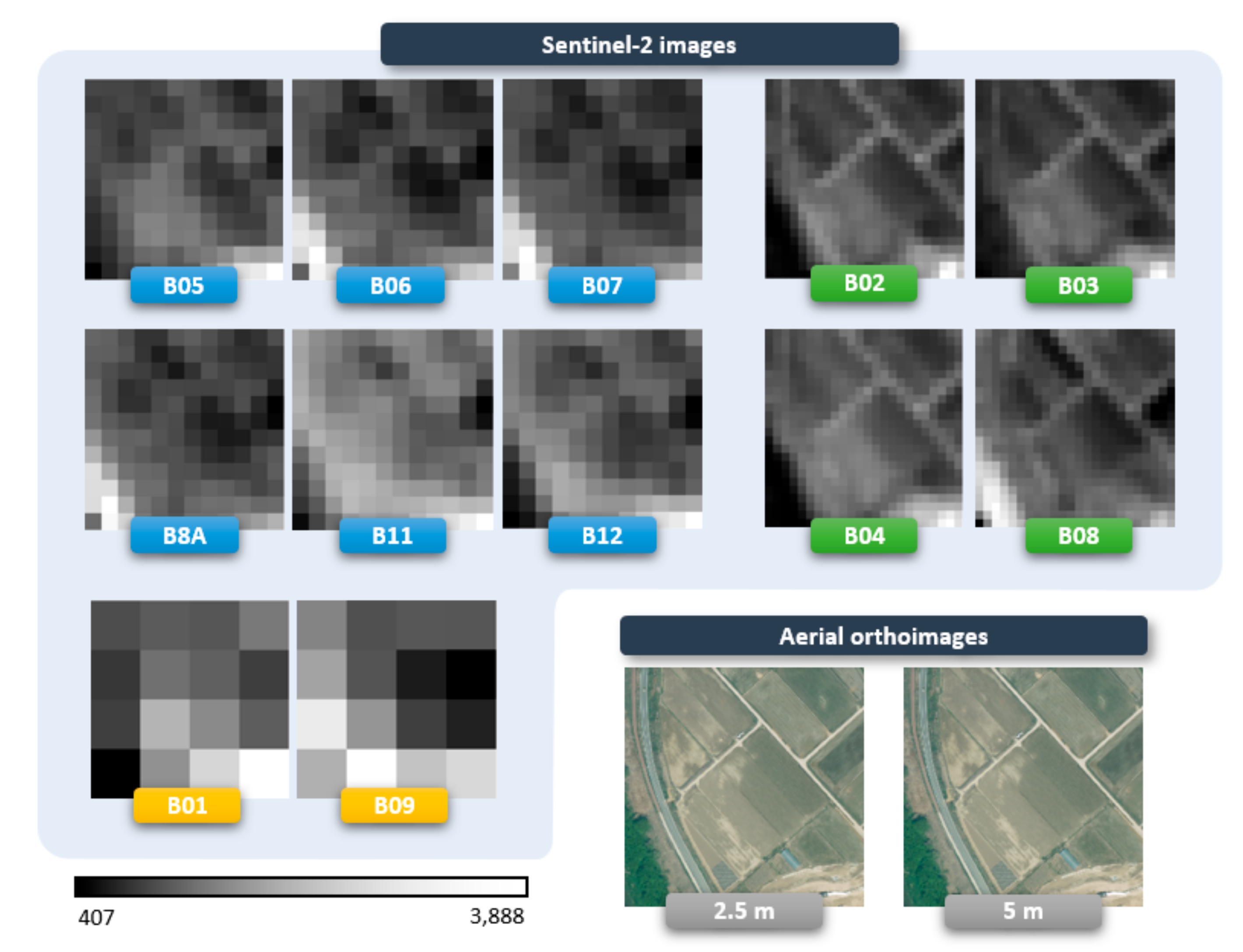
2.1.3. Sentinel-2A/B Satellite Imagery

Sentinel-2 is one of the satellites operated by the European Space Agency (ESA) and provides 13 multispectral bands with several different resolutions (10 m, 20 m, and 60 m). The imagery of Sentinel-2 has the highest resolution of 10 m among the current freely available for the general public. Accordingly, Sentinel-2 was selected for the study because it can provide much richer information than any other free satellite images. A short revisit period of five days is another strength of the Sentinel-2 imagery. Initially, the revisit period was ten days, but two satellites named Sentinel-2A and Sentinel-2B take images alternately, which reduces the revisit period to 5 days.

Sentinel-2 provides two types of images: (1) the L1C product, a top of atmosphere (TOA) reflectance image and (2) the L2A product, a bottom of atmosphere (BOA) reflectance image. The L2A product can overcome a significant difference in reflectivity, which varies for different acquisition times. Because aerial images are acquired at a much lower altitude than satellite images, it is better to use images with atmospheric correction. Because ESA provides the L1C product for images over the study area from 2018, all experimental images were converted to L2A through the Sen2cor tool of the Sentinel application platform (SNAP) software [9,13]. Twelve images (four 10 m, six 20 m, and two 60 m) with different spectral bands ranging from visible wavelength to SWIR were acquired. In some land classification studies, 60 m resolution images are not used because they are primarily for atmospheric correction [14,15]. However, we tested our approach with and without 60 m resolution imagery to consider whether additional atmospheric information is useful for training input images.

For matching the Sentinel-2 images acquired at the same time interval as the aerial orthoimages, data were searched through the Copernicus website, where the Sentinel series took all provided images [16]. We obtained both Sentinel-2A and 2B sensor images, which contain less cloud coverage, from the website. Searched images used in this research are listed in

Table 1. Sentinel-2 sensing start times used for the research.

Platform	Sensing Start Time
Sentinel-2A	2018/04/18 02:16:01
	2018/04/28 02:16:11
	2018/05/28 02:16:51
Sentinel-2B	2018/05/23 02:16:49
Total	4 images

, and only band 2 images are depicted in Figure 3. All 10 m and 20 m images were used in training as defaults, with 60 m as optional. Because the datasets are acquired simultaneously with the aerial orthoimages, it was assumed that there were no significant topographic changes during the short period. Accordingly, listed datasets are used for all the following experiments.

2.1.4. Training Datasets Generation

The training datasets were preprocessed based on 2.5 m downsampled aerial orthoimages and 10 m Sentinel-2 satellite images. The first step was to transform both image sets into the same map projection system. All image sets in this study were projected into the Korea 2000 coordinate system (EPSG: 5186), corresponding to transverse mercator (TM) projection. The second step was to determine the size of training datasets based on 60 m Sentinel-2 images. After considering the computational efficiency of training processes, the 4 × 4 pixels image size was used, corresponding to 240 × 240 m² on the ground. For this configuration, the image size for 2.5 m and 5.0 m aerial orthoimages were 96 × 96 pixels and 48 × 48 pixels, respectively. For the same reason, the training image sizes of 10 m and 20 m resolution for Sentinel-2 were 24 × 24 pixels and 12 × 12 pixels, respectively.

Training samples and test samples were selected randomly within the study area but did not overlap for the Daejeon area. Through this process, 32,632 training samples (6527 for validation samples, 20% of the training samples) and 8156 test samples were produced. In addition, 39,204 test samples were generated for the Sejong area. Each set consisted of twelve Sentinel-2 images (4 for 10 m, 6 for 20 m, and 2 for 60 m) and two aerial photographs (1 for 2.5 m and 1 for 5.0 m), as depicted in Figure 4. A 5.0 m aerial orthoimage was used as the GT for 2× magnification of 10 m Sentinel-2 images and 2.5 m for 4× magnification of 10 m Sentinel-2 images.

2.2. Methodology

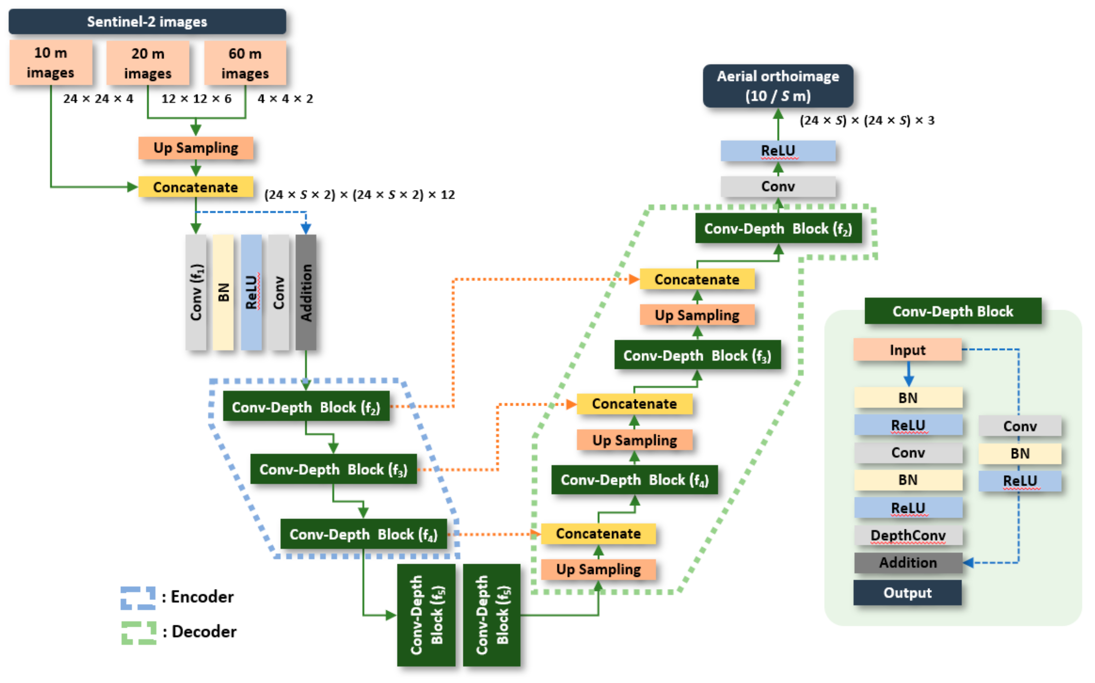
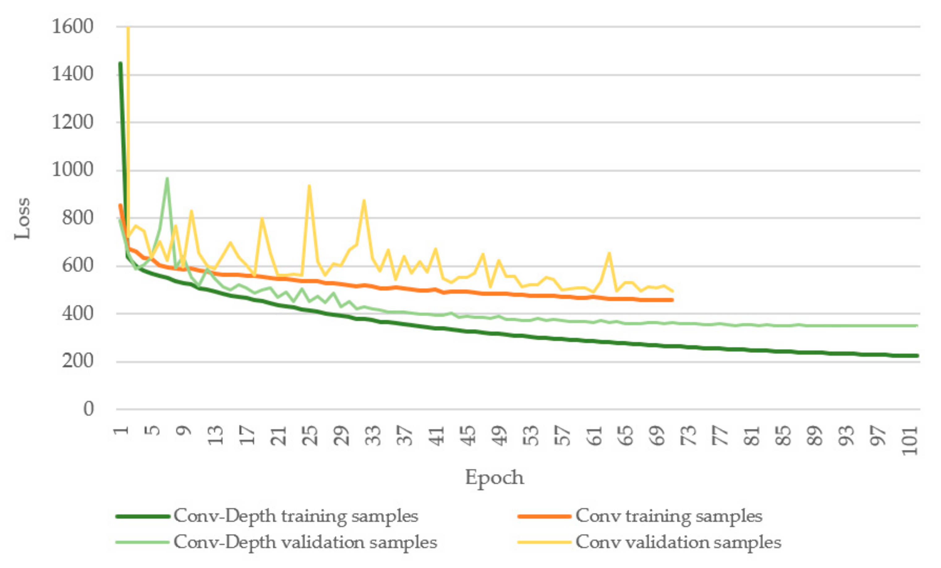
2.2.1. Context-Based ResU-Net

The latest research results indicate that the quality of SR increases as more convolution layers or deeper neural networks are assigned [6,8,9]. Most recent deep learning-based SR neural networks adopt this trend by maintaining the size of the input image until the output stage. The enlargement function to create HR is applied to the final stage [8,11,12]. The existing methodology was applied to our datasets with unsatisfactory results. It is speculated that different imaging geometry between aerial and space-borne sensors may lead to unsatisfactory results even with similar research methods. Because the aerial orthoimage contains more context information than the space-borne Sentinel-2 image, we determined that it would be critical to arrange context-preserving and deep and dense neural networks in the initial stage. The proposed architecture of the context-based ResU-Net for our study is depicted in Figure 5.

In our study, the residual U-Net proposed by Zhang et al. [17] was modified to maintain the context information and build deep neural networks. Batch normalization (BN) and ReLU activation functions are included in most of the steps. BN helps to solve gradient vanishing/exploding and overfitting caused by the deep neural network; it also improves accuracy [6,11]. The ReLU is used to remove the values below zero [6]. The encoder’s role is to make the input image compact, and the decoder recovers the information to generate the final image. There is a path connecting the encoder and the decoder, and all convolution layers have a filter size of 3 × 3. The encoding path has three conv-depth blocks. Each block’s stride was set to 2 instead of using downsampling layers to reduce the feature map’s size in half. The decoding path has three conv-depth blocks to correspond to the encoder, and the size is increased through upsampling layers. End of the decoding path, a convolution layer is inserted to make feature dimensions as 3 with ReLU activation function for generating desired resolution similar to that of aerial orthoimage.

There are three major differences between the existing Residual U-Net and our network. First, the conv-depth block was included to reduce computation resources. It is known that depth-wise separable convolution (DepthConv) maintains performance while reducing the number of parameters [18]. As shown in

Table 2. Comparison of parameter numbers.

Feature Dimensions	Compositions	Number of Parameters
		Trainable Parameters	Total Parameters
fa	Using convolutional layer only	4,718,035	4,725,331
	Using DepthConv layer	3,159,955	3,167,251
fb	Using convolutional layer only	18,845,091	18,859,683
	Using DepthConv layer	12,595,491	12,610,083
fc	Using convolutional layer only	75,326,275	75,355,459
	Using DepthConv layer	50,293,315	50,322,499

, if a convolution layer is used instead of a DepthConv layer in our architecture, the number of parameters to be learned becomes larger. In addition, the difference in the number of parameters increased as the size of the feature dimensions increased. Moreover, we had encountered that the validation loss was jagged when only the convolution layer was used. On the contrary, the loss converges evenly with a lower value when using the DepthConv layer, as shown in Figure 6. When only the convolution layer was used, the loss at epoch 1 was 45,328.06, but the value was too large to be displayed on the graph, so only the corresponding value was clipped.

Second, upscaling was applied in the initial stage of the neural networks. The reason for changing the order like this is that the final prediction image becomes smoother or darker than that of the GT image when the image size is enlarged in the final stage as most of the other SR networks are arranged. In our networks, the scale (S) indicates an increasing factor of the original image. For example, the scale was set to 2S at the beginning and halved at the end, achieving a double improvement effect. Finally, the stride parameter was set to 2 to halve the image resolution.

Third, the feature dimension (f = {f₁, f₂, f₃, f₄, f₅}) was configured to increase gradually as the image size decreases, and the experiment was conducted in three groups: f_a = {16, 32, 64, 128, 256}, f_b = {32, 64, 128, 256, 512}, and f_c = {64, 128, 256, 512, 1024}. It was designed to analyze the predictive ability according to the size of feature dimensions.

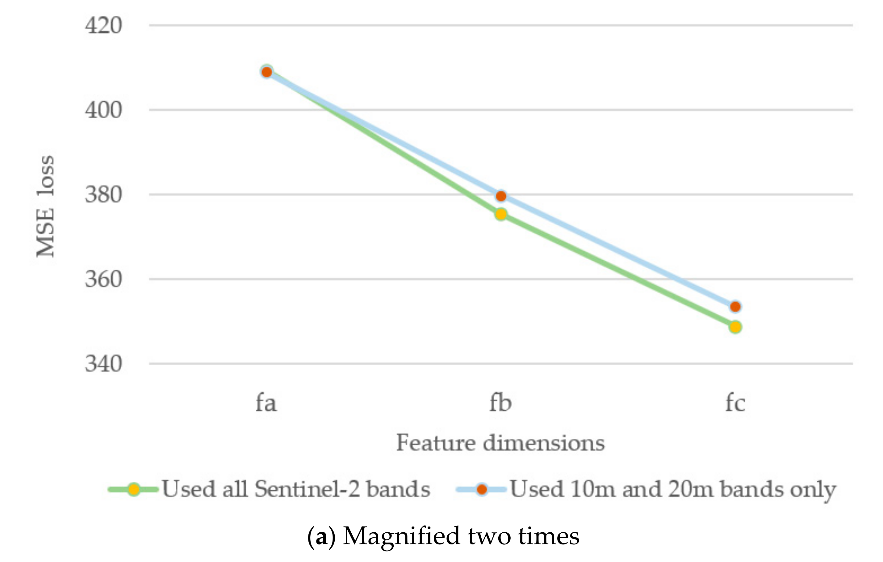
2.2.2. Hyperparameter Optimization

The following hyperparameters were chosen to control the learning process. The related parameters were the optimizer, loss function, learning rate, batch size, and epoch. For an optimizer Adam optimizer for gradient descent was used in this study, reflecting many previous studies that this optimizer produced the best performance and had lower memory requirements than others [6,9,10,19]. The L1 loss function was used to minimize the error, which is the sum of all the absolute differences between the true value and the predicted value; it has been widely applied to SR neural networks [11,12,19]. For our study, we adopted the mean squared error (MSE) loss function instead of L1 because MSE had better results than L1. Finally, the mini-batch size was set to 32.

The learning rate gradually decreased as the epoch increased through a rate decay scheduler [18]. Consequently, the learning rate functions as an essential hyperparameter because it is dependent on the epoch parameter. Therefore, the epoch was adjusted between 30 and 180 to find the minimum loss; the experiment was repeated for each model. The initial learning rate was set to 5 × 10^-4. Early stopping criteria using validation datasets were also applied to avoid overfitting, and learning was stopped if the accuracy was not improved within 10 epochs. All programming was performed with Python-based Tensorflow nightly (2.5.0) GPU version, and learning was conducted using three graphics cards: two GeForce RTX-2080 Ti (11 GB VDRAM) and one RTX-3090 (24 GB VDRAM).

3. Results

Two experiments were conducted to evaluate our results: (1) whether to use 60 m images and (2) the effects of the feature dimension sizes. The EDSR neural network was also trained for comparison with our results. EDSR was selected as a comparison due to its excellent performance among the currently developed SR neural networks [12]. Lim et al. [11] designed both baseline and EDSR models. The difference between the two models is the number of residual blocks and the feature dimension. The baseline model is organized with 16 residual blocks and 64 feature dimensions, and EDSR is formed with 32 residual blocks and 256 feature dimensions. Both models are utilized for comparison, and all related training parameters were set as the author suggested. After training both neural networks with the same datasets, the results were evaluated with three metrics. PSNR and SSIM were used to evaluate the outcome—they are most frequently used as an evaluation index of SR deep learning research [11,12,20]. The RMSE used in some studies [6,9] was also included. The comparison of the final three metrics is summarized in

Table 3. Quality evaluation results with set parameters for Daejeon City. Blue indicates the best results, and red indicates the second best.

Scale	Neural Networks	Use of 60 m	Feature Dimensions	Epoch	RMSE	PSNR	SSIM
2	Baseline (EDSR)	Y	64	120	22.9871	22.2210	0.4750
		N		100	23.1250	22.1883	0.4738
	EDSR	Y	256	70	22.5078	22.3772	0.4834
		N		100	21.9486	22.6070	0.4935
	Context-based ResU-Net (Ours)	Y	fa	180	20.2371	23.3116	0.5010
			fb		19.3775	23.6701	0.5233
			fc		18.6816	23.9578	0.5437
		N	fa		20.2274	23.3333	0.5005
			fb		19.4900	23.6332	0.5234
			fc		18.8066	23.8895	0.5439
4	Baseline (EDSR)	Y	64	180	24.6372	21.5330	0.3675
		N			24.7514	21.5305	0.3648
	EDSR	Y	256	30	26.4536	20.9607	0.3516
		N		40	26.7308	20.9715	0.3572
	Context-based ResU-Net (Ours)	Y	fa	180	22.9141	22.1295	0.3770
			fb		22.1827	22.3758	0.3888
			fc	120	21.3574	22.6966	0.4101
		N	fa		22.9897	22.1006	0.3774
			fb		22.1444	22.3971	0.3912
			fc		21.7778	22.5278	0.4018

for Daejeon City and

Table 4. Quality evaluation results for Sejong City. Blue indicates the best results, and red indicates the second best.

Scale	Neural Networks	Use of 60 m	Feature Dimensions	RMSE	PSNR	SSIM
2	Baseline (EDSR)	Y	64	30.3523	19.3793	0.4034
		N		30.5805	19.3052	0.4009
	EDSR	Y	256	30.3873	19.4050	0.4086
		N		30.0645	19.4856	0.4110
	Context-based ResU-Net (Ours)	Y	fa	30.4532	19.4819	0.4125
			fb	30.8639	19.3829	0.4122
			fc	30.4220	19.5121	0.4182
		N	fa	30.5115	19.4902	0.4183
			fb	30.3297	19.5689	0.4173
			fc	30.4948	19.5190	0.4151
4	Baseline (EDSR)	Y	64	31.5568	18.9689	0.3287
		N		31.4554	18.9719	0.3270
	EDSR	Y	256	32.4436	18.7164	0.3188
		N		33.1779	18.5482	0.3250
	Context-based ResU-Net (Ours)	Y	fa	31.3203	19.0943	0.3357
			fb	31.5619	19.0178	0.3357
			fc	31.6259	19.0225	0.3387
		N	fa	31.8976	18.9556	0.3368
			fb	31.4533	19.1072	0.3382
			fc	31.3686	19.0990	0.3407

for Sejong City, respectively. The scale parameters 2 and 4 refer to generating 5.0 m and 2.5 m aerial orthoimages, respectively.

In the case of Daejeon City, our context-based ResU-Net outperformed the baseline and EDSR models for all three metrics. For EDSR, even if the residual blocks and feature dimensions increased comparing with the baseline model, it is difficult to find performance improvement. In the case of Sejong City, in which independent testing was performed, our models performed better in two metrics except for RMSE.

The image quality deteriorated as the magnification was enlarged, and the value of the evaluation metrics gradually deteriorated. Through fine-tuning, the inclusion of 60 m images performs better in two networks. When 60 m images were included, RMSE decreased, and PSNR and SSIM increased. This result demonstrates that the 60 m images have a positive impact on both networks.

The loss converged to a lower value if feature dimensions increased, as depicted in Figure 7. The result also validated that the denser the neural network, the higher the quality. Moreover, we found the accuracy is much higher when both denser feature dimensions and the 60 m images were used.

For a visual comparison between EDSR and context-based ResU-Net, the prediction images are listed in

Table 5. Predicted images of Sentinel-2 and corresponding GT image (paddy/road area).

Scale	Use of 60 m	Predicted Images				Input Images per Each Resolution (Sentinel-2)
		Baseline and EDSR		Context-Based ResU-Net (Ours)
2	Yes	64		fa		< Band 01 (60 m) > < Band 02 (10 m) > < Band 05 (20 m) >
				fb
		256
				fc
	No	64		fa
				fb		GT image
						< Orthoimage (5.0 m) >
		256
				fc
4	Yes	64		fa		< Band 01 (60 m) > < Band 02 (10 m) > < Band 05 (20 m) >
				fb
		256
				fc
	No	64		fa
				fb		GT image
						< Orthoimage (2.5 m) >
		256
				fc

,

Table 6. Predicted images of Sentinel-2 and corresponding GT image (urban area).

Scale	Use of 60 m	Predicted Images				Input Images per Each Resolution (Sentinel-2)
		Baseline and EDSR		Context-Based ResU-Net (Ours)
2	Yes	64		fa		< Band 01 (60 m) > < Band 02 (10 m) > < Band 05 (20 m) >
				fb
		256
				fc
	No	64		fa
				fb		GT image
						< Orthoimage (5.0 m) >
		256
				fc
4	Yes	64		fa		< Band 01 (60 m) > < Band 02 (10 m) > < Band 05 (20 m) >
				fb
		256
				fc
	No	64		fa
				fb		GT image
						< Orthoimage (2.5 m) >
		256
				fc

,

Table 7. Predicted images of Sentinel-2 and corresponding GT image (forest area).

Scale	Use of 60 m	Predicted Images				Input Images per Each Resolution (Sentinel-2)
		Baseline and EDSR		Context-Based ResU-Net (Ours)
2	Yes	64		fa		< Band 01 (60 m) > < Band 02 (10 m) > < Band 05 (20 m) >
				fb
		256
				fc
	No	64		fa
				fb		GT image
						< Orthoimage (5.0 m) >
		256
				fc
4	Yes	64		fa		< Band 01 (60 m) > < Band 02 (10 m) > < Band 05 (20 m) >
				fb
		256
				fc
	No	64		fa
				fb		GT image
						< Orthoimage (2.5 m) >
		256
				fc

,

Table 8. Predicted images of Sentinel-2 and corresponding GT image (urban/forest area).

Scale	Use of 60 m	Predicted Images				Input Images per Each Resolution (Sentinel-2)
		Baseline and EDSR		Context-Based ResU-Net (Ours)
2	Yes	64		fa		< Band 01 (60 m) > < Band 02 (10 m) > < Band 05 (20 m) >
				fb
		256
				fc
	No	64		fa
				fb		GT image
						< Orthoimage (5.0 m) >
		256
				fc
4	Yes	64		fa		< Band 01 (60 m) > < Band 02 (10 m) > < Band 05 (20 m) >
				fb
		256
				fc
	No	64		fa
				fb		GT image
						< Orthoimage (2.5 m) >
		256
				fc

and

Table 9. Predicted images of Sentinel-2 and corresponding GT image (urban/road area).

Scale	Use of 60 m	Predicted Images				Input Imagesper Each Resolution (Sentinel-2)
		Baseline and EDSR		Context-Based ResU-Net (Ours)
2	Yes	64		fa		< Band 01 (60 m) > < Band 02 (10 m) > < Band 05 (20 m) >
				fb
		256
				fc
	No	64		fa
				fb		GT image
						< Orthoimage (5.0 m) >
		256
				fc
4	Yes	64		fa		< Band 01 (60 m) > < Band 02 (10 m) > < Band 05 (20 m) >
				fb
		256
				fc
	No	64		fa
				fb		GT image
						< Orthoimage (2.5 m) >
		256
				fc

. Each table shows the predicted image of one representative input Sentinel-2 image per resolution (10 m, 20 m, and 60 m) for two scales, 2 and 4. The 2.5 m and 5.0 m aerial orthoimages are GT. The use of the 60 m Sentinel-2 images is shown in the second column. The predicted images of the baseline and EDSR model are shown in the third column. There is not much difference between the baseline and EDSR model, and only EDSR will be compared in the following. The predicted images of our context-based ResU-Net for three feature dimensions (f_a, f_b, f_c) are shown in the fourth column of each table. Generally, the prediction images between EDSR and context-based ResU-Net are visually similar when the feature dimension of context-based ResU-Net is f_a. For EDSR, even if the residual blocks and feature dimensions increase, no further improvement can be found. However, in our model, as networks become denser from f_a to f_c, it can be seen that the prediction images are getting close to GT.

Observing the boundaries of an object reveals the difference between the two methods. For EDSR, when the image was enlarged four times, the overall boundary of each object remained similar or smoother than that of two-time enlargement-causing the prediction images to look blurry. For context-based ResU-Net, boundaries of each object became more distinct as the feature dimensions increased in density regardless of the enlargement scale. When the feature dimension reached its maximum size, the boundaries of the object became sharpest. Consequently, the visibility of all images improved.

Some differences were found between the two models. EDSR predicts a darker image, especially in forest areas (Table 7), and it produced a blurry image compared to ours, as shown in Table 5, Table 6, Table 7, Table 8 and Table 9. Interestingly, the result of context-based ResU-Net predicts even urban shadows well in the densest feature dimension f_c, which are not even expressed in EDSR as shown in Table 6. It was also identified that our model generally trained the boundaries of objects better. In particular, road boundaries are well preserved even the width is narrower than the 10 m resolution Sentinel-2 image. The result implies that the recognition of the object of concern, such as the road, can be possible by using predicted Sentinel-2 imagery, as shown in Table 5 and Table 7. The road boundaries become clear as feature dimension becomes denser, but it seems that some attention needs to be paid to the shape of the road for the inclusion of 60 m Sentinel-2 imagery. Some of the road boundaries were visually curved when the 60 m Sentinel-2 images were included, but they were straight when the 60 m image was not included. It can be said that there exists a tradeoff between the value of metrics and visualization when the road boundaries are concerned.

4. Discussion

A study was conducted to produce 2.5 m and 5.0 m resolution imagery with 10 m Sentinel-2 satellite images using aerial orthoimage as a ground truth. For this, training samples were produced by acquiring Sentinel-2 satellite images and aerial orthoimages over the same area and period. The training samples were used to simulate 2.5 m and 5.0 m aerial orthoimages. For quality check and general applicability of our neural network, additional test samples in an independent region were utilized. For producing better-simulated images, a new context-based neural network was proposed and compared with the existing neural network. Our context-based ResU-Net generally outperformed the baseline and EDSR for all three metrics, both in training samples and test samples. We believe that this is because conv-depth blocks helped the stability of our model. In any case, the utility of our model for successfully predicting narrow roads will be very high. Meanwhile, in order to improve the performance compared to the present, the obstacles to be solved were speculated as follows:

First, the effect of shadows in HR aerial images was significant. The Sentinel-2 images were acquired with a low-resolution at high altitude, whereas aerial images were acquired with HR at low altitude. Even in the same area, when images were acquired at a low altitude, the effect of shadows was much more prominent than at a high altitude. Because most of our study area included urban landscapes, the effect of shadows on HR images was much greater than for high altitude images. The original 51 cm aerial orthoimage was resampled to obtain GT using bilinear interpolation. During the bilinear interpolation process to create GT from the original 51 cm aerial orthoimage, the effect shadow smeared into other features and worsened the SSIM metric.

Second, there existed the effects of color correction during the composition of aerial orthoimages. The primary purpose of aerial orthoimages distributed by the Korean government is to produce a visually attractive map for the general public. We speculated that the original reflectance information had been corrected to make the orthoimage more pleasing, leading to potentially difficult and inaccurate training due to the use of aerial orthoimages.

For this study, it is essential that both aerial orthoimages and satellite images must be taken at a similar period of time. Recently, some countries have provided aerial orthoimages, so if researchers can check the acquisition date of aerial orthoimages, we expect that our research results can be utilized.

In future research, steps for shadow identification and shadow removal must be included based on deep learning, especially when using the HR aerial images as training sets. In the remote sensing community, CNN-based SR research is ongoing. However, several studies have tried to combine images obtained from multiple sensors to produce new images. We believe that the method and results presented in this study can contribute new insights for researchers performing similar studies.

References

1. National Geographic Information Institute National Territory Information Platform. Available online: http://map.ngii.go.kr/mn/mainPage.do (accessed on 31 December 2020).
2. Rahmani, S.; Strait, M.; Merkurjev, D.; Moeller, M.; Wittman, T. An adaptive IHS pan-sharpening method. IEEE Geosci. Remote Sens. Lett. 2010, 7, 746–750. [Google Scholar] [CrossRef] [Green Version]
3. Ghadjati, M.; Moussaoui, A.; Boukharouba, A. A novel iterative PCA–based pansharpening method. Remote Sens. Lett. 2019, 10, 264–273. [Google Scholar] [CrossRef]
4. Liebel, L.; Körner, M. Single-image super resolution for multi-spectral remote sensing data using convolutional neural networks. ISPRS-Int. Arch. Photogramm. Remote Sens. Spat. Inf. Sci. 2016, 41, 883–890. [Google Scholar] [CrossRef]
5. Gargiulo, M.; Mazza, A.; Gaetano, R.; Ruello, G.; Scarpa, G. A CNN-Based Fusion Method for Super-Resolution of Sentinel-2 Data. In Proceedings of the IGARSS 2018-2018 IEEE International Geoscience and Remote Sensing Symposium, Valencia, Spain, 22–27 July 2018; pp. 4713–4716. [Google Scholar]
6. Lanaras, C.; Bioucas-Dias, J.; Galliani, S.; Baltsavias, E.; Schindler, K. Super-resolution of Sentinel-2 images: Learning a globally applicable deep neural network. ISPRS J. Photogramm. Remote Sens. 2018, 146, 305–319. [Google Scholar] [CrossRef] [Green Version]
7. Shao, Z.; Cai, J.; Fu, P.; Hu, L.; Liu, T. Deep learning-based fusion of Landsat-8 and Sentinel-2 images for a harmonized surface reflectance product. Remote Sens. Environ. 2019, 235, 111425. [Google Scholar] [CrossRef]
8. Tai, Y.; Yang, J.; Liu, X. Image Super-Resolution via Deep Recursive Residual Network. In Proceedings of the IEEE Conference on Computer Vision and Pattern Recognition Workshops, Honolulu, USA, 21–26 July 2017; pp. 3147–3155. [Google Scholar]
9. Pouliot, D.; Latifovic, R.; Pasher, J.; Duffe, J. Landsat super-resolution enhancement using convolution neural networks and Sentinel-2 for training. Remote Sens. 2018, 10, 394. [Google Scholar] [CrossRef] [Green Version]
10. Galar, M.; Sesma, R.; Ayala, C.; Aranda, C. Super-Resolution for Sentinel-2 Images. In Proceedings of the International Archives of the Photogrammetry, Remote Sensing and Spatial Information Sciences—ISPRS Archives, Nanjing, China, 25–27 October 2019; Volume 42, pp. 95–102. [Google Scholar]
11. Lim, B.; Son, S.; Kim, H.; Nah, S.; Mu Lee, K. Enhanced Deep Residual Networks for Single Image Super-Resolution. In Proceedings of the IEEE Conference on Computer Vision and Pattern Recognition Workshops, Honolulu, USA, 21–26 July 2017; pp. 136–144. [Google Scholar]
12. Zhang, Y.; Li, K.; Li, K.; Wang, L.; Zhong, B.; Fu, Y. Image Super-Resolution Using Very Deep Residual Channel Attention Networks. In Proceedings of the European Conference on Computer Vision (ECCV), Munich, Germany, 8–14 September 2018; pp. 286–301. [Google Scholar]
13. Thanh Noi, P.; Kappas, M. Comparison of random forest, k-nearest neighbor, and support vector machine classifiers for land cover classification using Sentinel-2 imagery. Sensors 2018, 18, 18. [Google Scholar] [CrossRef] [PubMed] [Green Version]
14. Wang, Q.; Shi, W.; Li, Z.; Atkinson, P.M. Fusion of Sentinel-2 images. Remote Sens. Environ. 2016, 187, 241–252. [Google Scholar] [CrossRef] [Green Version]
15. Gašparović, M.; Jogun, T. The effect of fusing Sentinel-2 bands on land-cover classification. Int. J. Remote Sens. 2018, 39, 822–841. [Google Scholar] [CrossRef]
16. European Space Agency (ESA) Copernicus. Available online: https://scihub.copernicus.eu/dhus/#/home (accessed on 31 December 2020).
17. Zhang, Z.; Liu, Q.; Wang, Y. Road extraction by deep residual u-net. IEEE Geosci. Remote Sens. Lett. 2018, 15, 749–753. [Google Scholar] [CrossRef] [Green Version]
18. Chen, L.-C.; Zhu, Y.; Papandreou, G.; Schroff, F.; Adam, H. Encoder-Decoder with Atrous Separable Convolution for Semantic Image Segmentation. In Proceedings of the European Conference on Computer Vision (ECCV), Munich, Germany, 8–14 September 2018; pp. 801–818. [Google Scholar]
19. Sun, Y.; Xu, W.; Zhang, J.; Xiong, J.; Gui, G. Super-Resolution Imaging Using Convolutional Neural Networks. Lecture Notes in Electrical Engineering; Springer: Berlin/Heidelberg, Germany, 2020; Volume 516, pp. 59–66. [Google Scholar]
20. Dong, C.; Loy, C.C.; He, K.; Tang, X. Learning a Deep Convolutional Network for Image Super-Resolution. In Proceedings of the European Conference on Computer Vision, Zurich, Switzerland, 6–12 September 2014; Springer: Berlin/Heidelberg, Germany, 2014; pp. 184–199. [Google Scholar]
Figure 1. Location of Daejeon and Sejong depicted with Google map and Sentinel-2 images (band 2 image acquired on 2018/04/18).
Applsci 11 01089 g001
Figure 2. Aerial orthoimages over the study area with the acquisition date.
Applsci 11 01089 g002
Figure 3. Acquired Sentinel-2 band number 2 (10 m) images: (a) Sentinel-2A 2018/04/18, (b) Setntinel-2A 2018/04/28, (c) Setntinel-2A 2018/05/28, (d) Setntinel-2B 2018/05/23.
Applsci 11 01089 g003aApplsci 11 01089 g003b
Figure 4. Example of training sets (Input: {B2 B3 B4 B8}: 10 m, {B5 B6 B7 B8A B11 B12}: 20 m, and {B1 B9}: 60 m, output: aerial orthoimages 2× for 5.0 m, 4× for 2.5 m).
Applsci 11 01089 g004
Figure 5. Context-based residual U-net for aerial images simulation (S: scale, f: feature dimension).
Applsci 11 01089 g005
Figure 6. Loss convergence comparison: conv-depth block vs. conv only for context-based ResU-Net when using 60 m images with fc feature dimensions (2×).
Applsci 11 01089 g006
Figure 7. Convergence results according to each feature dimension.
Applsci 11 01089 g007aApplsci 11 01089 g007b