
A Hybrid Wind Power Forecasting Model with XGBoost, Data Preprocessing Considering Different NWPs


1
Department of Electrical Engineering, College of Engineering, National Chung Cheng University, Chiayi 62102, Taiwan
2
Faculty of Electronics and Electrical Engineering, Ho Chi Minh City University of Technology (HCMUT), 268 Ly Thuong Kiet Street, District 10, Ho Chi Minh City 70000, Vietnam
3
Vietnam National University Ho Chi Minh City, Vietnam Linh Trung Ward, Thu Duc District, Ho Chi Minh City 70000, Vietnam
*
Author to whom correspondence should be addressed.
Appl. Sci. 2021, 11(3), 1100; https://0-doi-org.brum.beds.ac.uk/10.3390/app11031100
Submission received: 29 December 2020
/
Revised: 19 January 2021
/
Accepted: 21 January 2021
/
Published: 25 January 2021
(This article belongs to the Special Issue Joint Issue with 5th International Symposium on Computer, Consumer and Control (IS3C2020))
Abstract
:In recent years, wind energy has become a competitively priced source of energy around the world, which has created increasing challenges for system operators. Accurate wind power generation forecasting plays an important role in power systems to improve the reliable and efficient operation. Therefore, numerous artificial intelligent methods such as machine learning and deep learning have been considered as solutions for accurate wind power forecasts. In addition to deterministic forecasting, the probabilistic forecasting becomes more important, because it indicates the level of uncertainty. In this paper, a hybrid forecasting model considering different Numerical Weather Prediction (NWP) models and the XGBoost training model is proposed for short-term wind power forecasting. The proposed forecasting algorithm includes data preprocessing, in which an autoencoder model is used to reduce the dimension of 20 NWP ensembles. The performance of the proposed method is investigated using historical wind power measurements and NWP results by the Taiwan Central Weather Bureau (CWB); the NWP includes spot wind speeds from WRFD, RWRF, and ensemble wind speeds from WEPS. Based on the forecasting results, the proposed model produces better performance and forecasting accuracy among other forecasting models, which reveals the importance of data preprocessing using autoencoders and the use of deep learning models in deterministic or probabilistic forecasts.
1. Introduction
Wind is one of the prominent renewable energy resources because it is more accessible, inexhaustible, fairly cheaper, environmentally friendly, and clean. In some regions where wind power resource is enormous, the yield of wind electricity begins to account for a significant proportion [1]. For instance, in Taiwan, about 6.5 GW of offshore wind power will be integrated by 2030. However, the generation of wind power is facing primary problems on its uncertainty and intermittency. Power fluctuations from wind turbines are caused by season, temperature, air pressure, and so on [2]. The variability of grid-connected wind power has led to numerous challenging tasks, including optimal unit scheduling, power system inertia, sizing of energy storage system, determination of energy reserves, energy market policies, and reliability assessment [3]. Power system inertia is important for maintaining grid stability. A power system with insufficient inertia can suffer from the problems on transient frequency stability. In the past, the primary resources for providing inertia come from synchronous generators. However, as the penetration of wind power generation increases, the rotating inertia contributed by synchronous generators could be reduced, increasing the risk of power system operations. Therefore, wind power forecasting (WPF) is one of the most efficient ways to reduce the uncertainty on power system operations.
Traditional single-value predictions, also called deterministic forecasting, cannot provide uncertainty information. By contrast, probabilistic forecasting is able to provide the set of potential values within which the observation is supposed to lie with a certain probability [4]. There are a variety of probabilistic wind power forecasting methods; they are divided into three main groups [5]: predicted error approach, direct approach, and approaches based on the NWP data. Traditional predicted error approaches were mainly divided into two techniques: parameter-based approach and bootstrap. Regarding the parameter-based approach, several studies described the forecasting uncertainty with suitable probability density functions (PDF) that are generated by historical forecasting errors. For example, Gaussian distribution or beta distribution is the most popular assumption for a PDF. The bootstrap approaches, such as the standard bootstrap, pair bootstrap, and moving block bootstrap, estimate the distribution of forecasting errors by resampling the original data, and an artificial intelligent model can be used to generate forecasting results. For the direct approach, the lower and upper bounds for prediction intervals are trained and constructed by artificial intelligent (AI) technologies. However, the AI model itself is not able to provide Predicted Intervals (PIs). To solve that problem, many developed optimizations were developed. For instance, the lower upper bound estimation (LUBE)-based neural network with a modified bat algorithm (MBA) [6] was used to maximize PI coverage probability (PICP) and minimize PI normalized average width (PINAW). Similarly, quantum-behaved particle swarm optimization (QPSO) was also utilized to optimize PIs [7].
In terms of NWP, spot NWP models consider the physical parameters of weather variables and are widely developed by meteorologists. Most commercial wind power forecasting methods utilized single-value NWP wind forecasts as input data [8,9]. Ensemble NWPs have been developed widely to provide an assessment of weather uncertainty by varying initial weather parameters in a lower resolution [10]. Moreover, reference [11] proved that the combination of deterministic and probabilistic models enhances wind power forecasts. In this work, NWP ensembles include 20 wind speed members, which would reduce the training speed of the model. Consequently, an autoencoders model was developed for dimensional reduction, which reduces the original NWP ensembles wind speeds and accelerates the model training.
Data preprocessing is one of the most important parts for wind power forecasting to extract the features [12,13], data modification [14], or dimension reduction [15]. The Weather Research and Forecasting (WRF) model is a next-generation mesoscale numerical weather prediction system. It includes deterministic WRF (WRFD), radar WRF (RWRF), and a WRF ensemble prediction system (WEPS). For short-term predictions, the inputs of the forecasting model can comprise historical wind power and different NWP results, including spot NWPs (WRFD and RWRF) and ensemble NWP (WEPS). Therefore, data preprocessing can be applied to wind power, WRFD, RWRF, and WEPS. Furthermore, there are numerous methods to increase the forecasting performance based on NWP adjustments [12,13].
This paper considers the short-term wind power forecasting, which is important for the intraday trading and the management of the transmission systems. Since the used NWP WEPS wind speeds are generated every three hours, thus, this paper considers the three-hour-ahead short-term wind power forecasting.
Additionally, this work develops a hybrid model for probabilistic wind power forecasting. It considers different NWP data, dimensional reduction for ensemble NWPs, and XGBoost. The forecasting module, i.e., prediction interval, in this work uses lower upper bound estimation based on Long Short-Term Memory (LSTM) [16,17,18]. According to the forecasting results, the proposed forecasting model outperforms traditional models in term of accuracy and reliability.
The rest of this paper is structured as follows. Chapter 2 is a literature review for wind power forecasting using NWP data. Chapter 3 provides a brief overview of assessment indices for deterministic and probabilistic forecasts to understand the forecast quality by its sharpness and reliability. Chapter 4 introduces the methodologies, including XGBoost and Autoencoders. Chapter 5 is the process of the proposed forecasting method. Chapter 6 provides the preprocessing of the dataset in the forecasting process. Chapter 7 introduces the proposed probabilistic forecasting model. Chapter 8 discusses the forecasting results among different methods. Chapter 9 gives the conclusion of this paper.
2. Literature Review for Wind Power Forecasts Using NWP Data
2.1. Overview of Wind Power Forecasting Methods
Wind power forecasts are classified by various methods according to time horizons or methodologies. The classification based on time horizon is different in various research studies. However, it can be divided mainly into four main categories:
- −
- Very short-term forecasting: from a few seconds to 30 min ahead; it is for real-time system operations.
- −
- Short-term forecasting: from 30 min to several hours ahead; it is for economic dispatch and load management.
- −
- Medium-term forecasting: from several hours to one day ahead; it is for unit commitment and electricity market operation.
- −
- Long-term forecasting: more than one day ahead; it is for power system risk assessment and energy planning.
In terms of forecasting methodologies, most of the wind power forecasting approaches are divided into persistence methods, Numerical Weather Prediction (NWP) methods, statistical methods, artificial intelligence methods, spatial correlation methods, and hybrid methods [19].
2.2. Numerical Weather Prediction (NWP)
NWP plays an important role in wind power forecasting. Thus, the inputs of the wind power forecasting model should involve NWP data. Figure 1 shows a typical probabilistic model for wind power generation based on the input of deterministic NWPs, in which both measured data from wind farms and deterministic NWPs are considered. NWP-based forecasts can be obtained either by prediction error approaches or direct approaches [20].
Many forecasting approaches with ensemble NWPs have been utilized to provide the probability of wind uncertainties. A typical ensemble NWP model may include a unique conversion model, multi-conversion forecasting model, or dimensional reduction model, as shown in Figure 2.
In [5], the authors used a dimensional reduction method to extract the features of ensemble NWP data and constructed a short-term probabilistic forecasting engine using a LUBE-based neural network. However, this work only considered a single NWP model. The study in [13] proposed an approach that improves short-term wind power forecasting by the combination of a K-means algorithm, artificial neural network, and Bayes information criterion that is used for identifying and mining bad data of NWPs. However, the proposed model includes many parameters, which requires a long time for computation and analyses in real applications. In [20], a hybrid approach was developed using K-means cluster analysis and a generalized regression neural network (GRNN) model that is based on NWP data. However, other advanced clustering methods may surpass the K-means algorithm and obtain better forecasting results.
All the above works considered the improvement of the input data before they are input into wind power forecasting models. This paper continued the previous work in [21] and improved the performance of probabilistic wind power forecasting considering various NWP models. Finally, a comprehensive analysis about the forecasting results was performed.
3. Assessment Indices for Deterministic and Probabilistic Forecasts
3.1. Root Mean Squared Error (RMSE)
A variety of statics have been proposed and employed to evaluate the forecast performance, but no single one is accepted as the universal standard [22]. There are many criteria for rating network effectiveness’s assessment, such as Root Mean Squared Error (RMSE), Mean Absolute Percentage Error (MAPE), Mean Squared Error (MSE), and Mean Absolute Error (MAE). All of those indexes have been utilized for deterministic forecasts. For a short-term wind power forecast, RMSE is generally chosen to be the comparison index among different methods, which can be illustrated by:
where n is the number of data, P0 is real-time power, and P is forecasting wind power.
3.2. Reliability: Prediction Interval Coverage Probability (PICP)
To avoid under- or over-confidence, the value PICP is determined to represent the percentage of observations or actual wind power values that fall within a range between lower bounds and upper bounds, where the subscript t refers to the number of a sample or a time step. Greater PICP implies that there are more targets in the corresponding PIs. PICP is calculated as follows:
where N is the total number of samples and ct is a Boolean value, which is defined as:
where yt, Lt, and Ut are the observation value, the lower bound, and the upper bound, respectively, with the same number of timestep t. A confidence level refers to the percentage of all possible samples that can be expected to include the real population parameter. For example, a 50% confidence level implies that 50% of the confidence intervals would include the real population parameter. Generally, PICP must be close to the confidence level that is predetermined in the probabilistic model.
3.3. Sharpness: Prediction Inteval Normalized Average Width (PINAW)
Obviously, widening the PIs leads to the increase of PICP, but it is not useful for decision-making. As a result, a measure of the average width of PIs, namely PINAW, is defined as:
where R is the range of underlying targets that are used to normalize predicted intervals.
3.4. Aggregative Index: Coverage Width Criterion (CWC)
PINAW and PICP represent the reliability and the sharpness of PIs, respectively. In fact, it is necessary to find an index that considers both aspects. Therefore, the CWC is the index that is used for this work. It is calculated as:
where μ is the confidence level for PIs. When μ is greater than PICP, a penalty coefficient η is activated to maximize the difference between PICP and μ. γ (PICP, μ) is described as follows:
CWC = PINAW(1 + γ(PICP, μ)e−η(PICP−μ))
4. Methodology
The major objective of this paper is to develop a new probabilistic wind power forecasting method, which is based on XGBoost, LUBE based on LSTM, and the preprocessing process by Autoencoder.
4.1. XGBoost
The decision tree is selected by XGBoost as its based learner [23]. The error between the predictive value and the target is reduced by adding more new based learners. Summation of all the base learners achieves the final predictive values. The XGBoost algorithm can be considered as an additive model consisting of M decision trees, which are given by:
where f is a decision tree, and F represents the function of all decision trees. In the regression process, the object function of the additive model becomes
where l denotes loss function and Ω is the regularization term.
Vector mapping is used to improve the decision tree for each regularization term Ω(f). Ω(f) can be represented by
where T indicates the number of a decision tree’s leaf nodes; ω represents the vector of score, and both γ and λ express the penalty factor.
XGBoost uses the forward stage-wise algorithm to simplify the complex of the model. Every time the model adds a decision tree, it learns a new function and its coefficients to fit the last step predicted residuals. Therefore, when the tth step learning happens, the predictive value of xi is . Therefore, the object function should be expressed by
The greedy algorithm is applied in the XGBoost model to build the decision tree; by building decision trees continually, a complete XGBoost model is established. Furthermore, the randomization technique is also implemented in XGBoost to reduce overfitting and increase training speed, and the sparsity-aware algorithm is used to effectively eliminate missing values from the computation of the loss gain of split candidates. Numerous parameters have been tuned for XGBoost in this work, which include the learning rate, the minimum sum of weights of all observations required in a child, the maximum depth of the tree, and the subsampling rate. These important parameters will be mentioned in Chapter 7. The process of tuning is to select the best parameters for an algorithm to optimize the performance.
4.2. Autoencoders
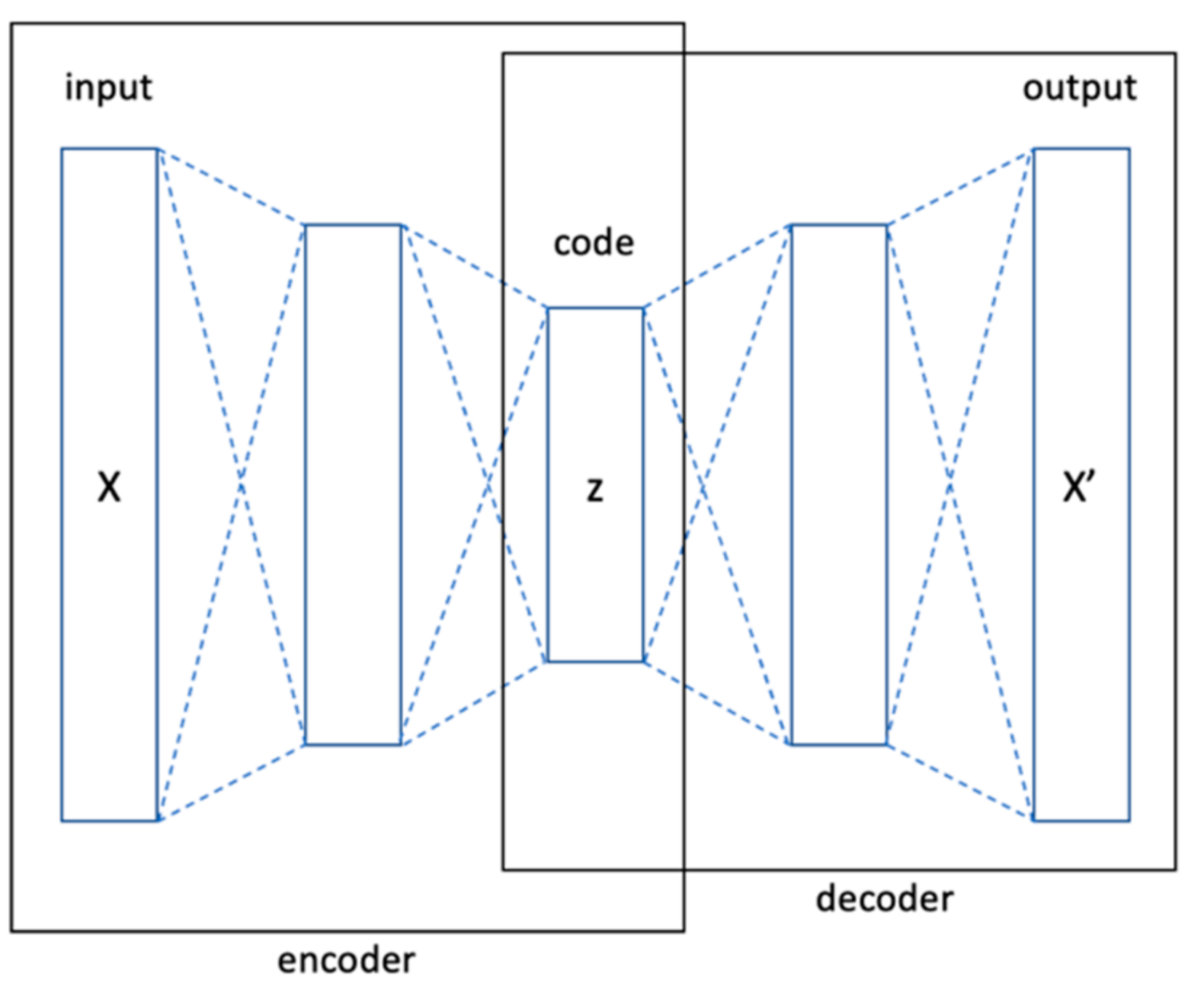
An autoencoder is a type of unsupervised artificial neural network (ANN), which compresses the data into a lower dimension and then reconstructs the input back. The autoencoder is trained to learn the representation of the input data in a lower dimension by focusing on the important features, getting rid of noise and redundancy. It is based on Encoder–Decoder architecture, as shown in Figure 3, where an encoder encodes the high-dimensional data and reconstructs the original high-dimensional data. Moreover, the autoencoders are feed forward deep learning models, which represents the learning flexibility [24,25,26].
The structure of an autoencoder is similar to that of a feedforward neural network (Multi-Layer Perceptron). In terms of its simplest form, an autoencoder uses hidden layers to recreate the inputs. The algorithm of an autoencoder is described in two parts:
Part 1: Encoder function (Z = f(X)) that converts X to Z codings.
Part 2: Decoder function (X’ = g(Z)) that produces a reconstruction of the inputs (X’).
The encoder and the decoder can be defined as transitions ϕ and ψ, such that:
In the simplest case, given one hidden layer, the encoder stage of an autoencoder takes the input and maps it to :
This image z is usually referred to as code. Hence, an element-wise activation function , for example, sigmoid or rectified linear unit, a weight matrix W, and a bias vector b. Weight and bias are normally initialized randomly and then updated iteratively during training through back-propagation. Then, the decoder stage of the autoencoder maps z to the reconstruction X’ of the same shape as x.
To reduce the dimension of the learning model, this study has reduced the size of the code that adequately represents X. An undercomplete autoencoder whose internal representation has a smaller dimensionality than the input data is represented in Figure 3.
To learn the neuron weights, the autoencoder seeks to minimize the loss function, such as RMSE, which penalizes X’ for being dissimilar from X:
5. Preprocessing of Datasets
Normally, data derived from the wind farm contain many outliers, noisy data, and missing values. These unreasonable data decrease the prediction accuracy. Data preprocessing can provide a strong preliminary interpretation of the dataset; consequently, data preprocess is the first stage in a typical forecasting algorithm.
- −
- Data cleaning: original data have many outliers, and these data are unreasonable and need to be cleaned.
- −
- Filling missing data: It is necessary to fill missing data while some measured wind data collected from the wind farm were lost. In this study, missing data are filled by linear interpolation. Thus, the accuracy of the forecasting model can be significantly improved.
- −
- Data normalization: Different variables have different units; that is, the process of data normalization is important. The following formula was used to transform all data values within the range 0 I:
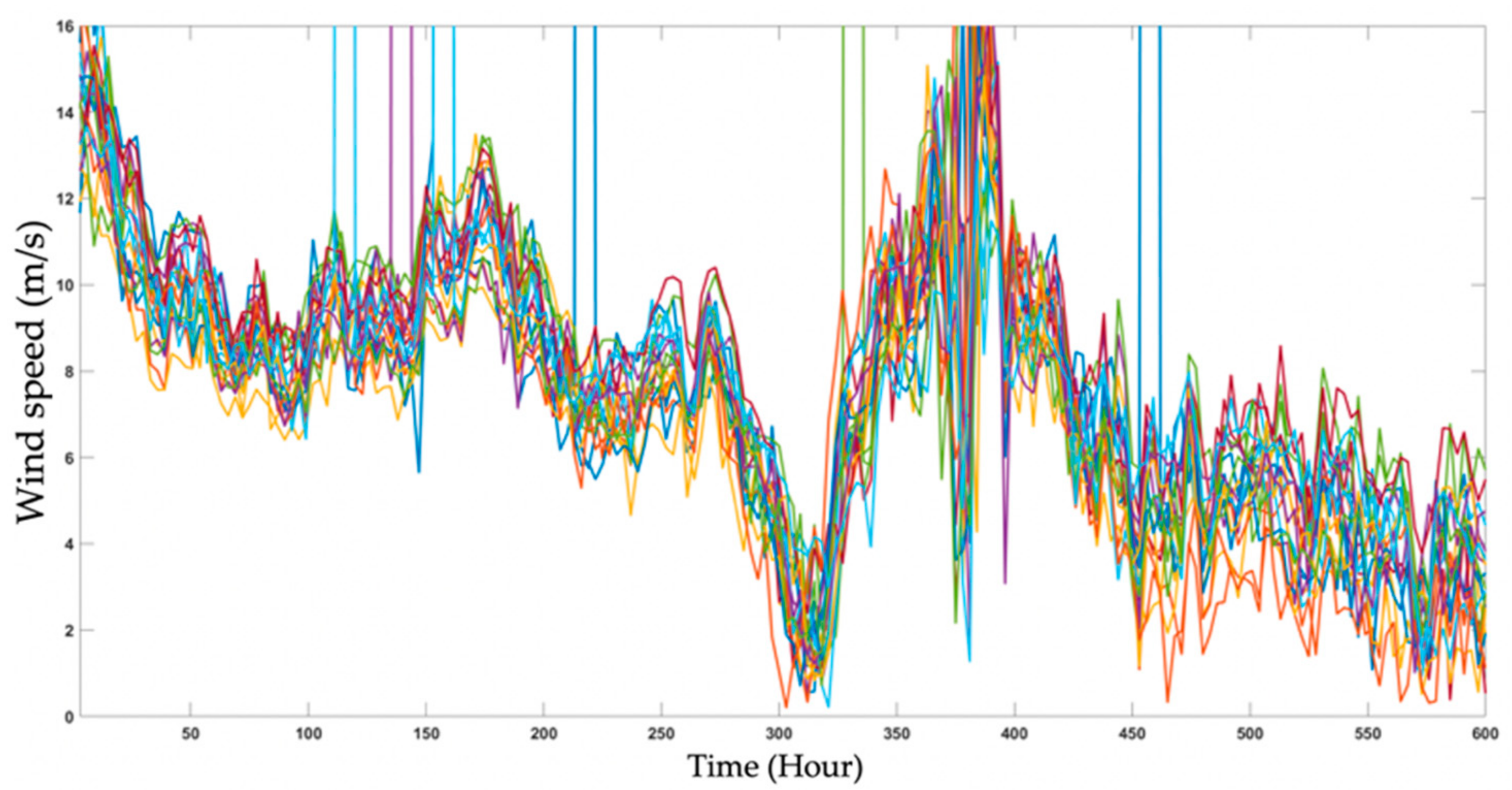
Every country has developed their own NWP systems, including global and regional models. This work utilizes historical wind power data recorded at Taiwan’s wind farms and the NWP wind-speed forecasts by Taiwan’s central weather bureau. The state-of-the-art NWP system is essential for the weather forecasts and climate applications. In particular, NWP also plays an important role in the application for renewable energy. The Taiwan CWB has developed the global and regional NWP systems for 30 years [21]. In this paper, three CWB NWP systems were used to evaluate the potential for forecasting wind power, which are called WRFD, RWRF, and WEPS. It consists of the complex model of WRF. In a WEPS model, it generates ensemble wind speeds (20 different NWP outputs) every three hours. An example of a 20-WEPS member of wind speeds is shown in Figure 4.
The proposed dimensional reduction module is called the autoencoder-based deep learning method. The lower-bound and upper-bound NWP values are obtained from 20 members of ensemble wind speeds by dimensional reduction. It converts 20 NWP ensemble values to two values (lower and upper bound) to enhance the forecasting accuracy. The autoencoder is trained using both encoder and decoder. To obtain the dimension reduction, the layer between the encoder and decoder is set to two. Then, the middle layer is used as an output layer, as shown in Figure 5. Figure 6 shows the overall results after the preprocessing process, which points out the accuracy and stability of the new dataset. In this study, high dataset stability is defined if the data go through the processes of removing noises, filling missing data, and using the algorithm of the autoencoder. These processes are critical to improve the performance of a forecasting model.
6. The Structure of Proposed Model for Probabilistic Wind Power Forecasting
Figure 7 shows the proposed 3 h-ahead probabilistic wind power forecasting model. There are three main processes: preprocessing of dataset, deterministic wind power forecasting using XGBoost, and probabilistic wind power forecasting based on LUBE-LSTM (Lower Upper Bound Estimations–Long Short-Term Memory) model. The LUBE method was selected because it is advantageous to wind power forecasting; several previous studies [5,6,27] have verified its effectiveness on forecasts. LUBE can be directly constructed using the LSTM model, enabling predictors to select more input variables and generate two outputs (lower and upper bounds). For probabilistic forecasts, lower bound and upper bound are significant to build PIs.
The outputs of the LUBE-LSTM model provide a lower bound and upper bound on wind power forecasts. Figure 8 depicts the overall steps of the proposed forecasting method. There are nine steps for the proposed forecasting method.
- Step 1:
- The input data include historical wind power measurements, spot NWPs (WRFD, RWRF), and NWP ensemble wind speeds (WEPS).
- Step 2:
- Splitting data into a training set and testing set, the dataset is shown in Table 1.
- Step 3:
- Since the value of wind speeds varies dramatically, the normalization must be used for calibrating them into the range of zero to unity.
- Step 4:
- The preprocessing process for the original data includes a dimension reduction using autoencoder and wind power curve calibration. The detail about the calibration of a wind power curve was proposed in our previous work [21]. In real operations, wind power curtailment is commonly implemented by wind farm operators because of some emergency conditions, resulting in deviations from a normal power curve. For instance, the manual operation of wind turbines by operators sometimes reduces wind power generation. However, in the process of model training, these abnormal operating points should be removed to avoid training errors.
- Step 5:
- Deterministic forecasting is implemented every 3 h by XGBoost, as shown in Figure 9.
- Step 6:
- Tuning parameters after training model by XGBoost.
- Step 7:
- Obtain all of the errors from previous generated power. Then, construct the probability density function (PDF) of the errors. The lower bound and upper bound are obtained from the forecasting errors, which are associated with the highest probability. Next, compute the lower and upper bounds of the produced power as follows:where Eup and Elow are the upper bound and lower bound of the forecasting errors, respectively; WPup and WPlow are the upper bound and lower bound outputs of the LSTM model; and WPforecast is the deterministic forecasting obtained from the XGBoost model.
- Step 8:
- Train the model with the above lower and upper bounds of wind power as the output. Different inputs are shown in Figure 10. The data in February were used for prediction, and the data in January were used as validation data. The historical data from July 2019 to December 2020 were used as the training data.
- Step 9:
- The performance of the model is assessed by using the mentioned criteria, i.e., PICP, PINAW, and CWC.
7. Forecasting Results
In this work, the proposed forecasting model was applied to the Hu-Si wind farm on Penghu Island, Taiwan. The Hu-Si wind farm has six wind turbines, and the capacity of each turbine is 0.9 MW.
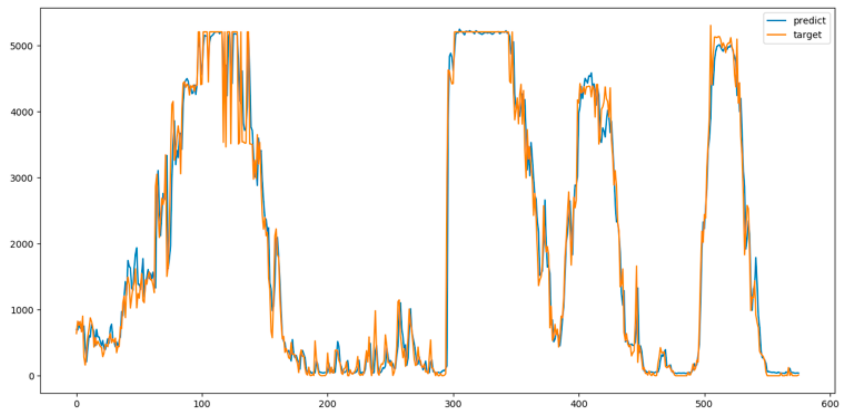
Figure 11 shows the three-hour-ahead deterministic forecasting results by XGBoost with data preprocessing and tuned parameters. Table 2 lists four important parameters in the XGBoost model. Accordingly, the blue line in Figure 11 denotes forecasting values, while the orange line stands for actual values.
It can be seen clearly that the proposed XGBoost approach can track the actual data well. The error created from the proposed XGBoost is small; the RMSE on the training set and forecasting set are 0.177 MW and 0.352 MW, respectively.
To demonstrate the superiority of the proposed method, the forecasting results by the proposed method are compared with those by other forecasting models:
- −
- Method 1a,b: Proposed model with different NWPs scenarios: (a) RWRF and WEPS, (b) WRFD and WEPS.
- −
- Method 2: XGBoost with standard dimension reduction.
- −
- Method 3: ANN model with standard dimension reduction.
Method 1a,b was selected in order to demonstrate the importance for considering various NWP models. This study focuses on the importance of various NWP methods on wind power forecasting. In the proposed method, the inputs include WRFD, RWRF, and WEPS, while the inputs of Method 1a only include RWRF and WEPS, and the inputs of Method 1b include WRFD and WEPS. The purpose for distinguishing different NWP inputs is to demonstrate and compare the forecasting results by considering different NWP models; Method 2 was selected to highlight the importance of the dimension reduction technique; Method 3 was selected to reveal the importance of the training AI method.
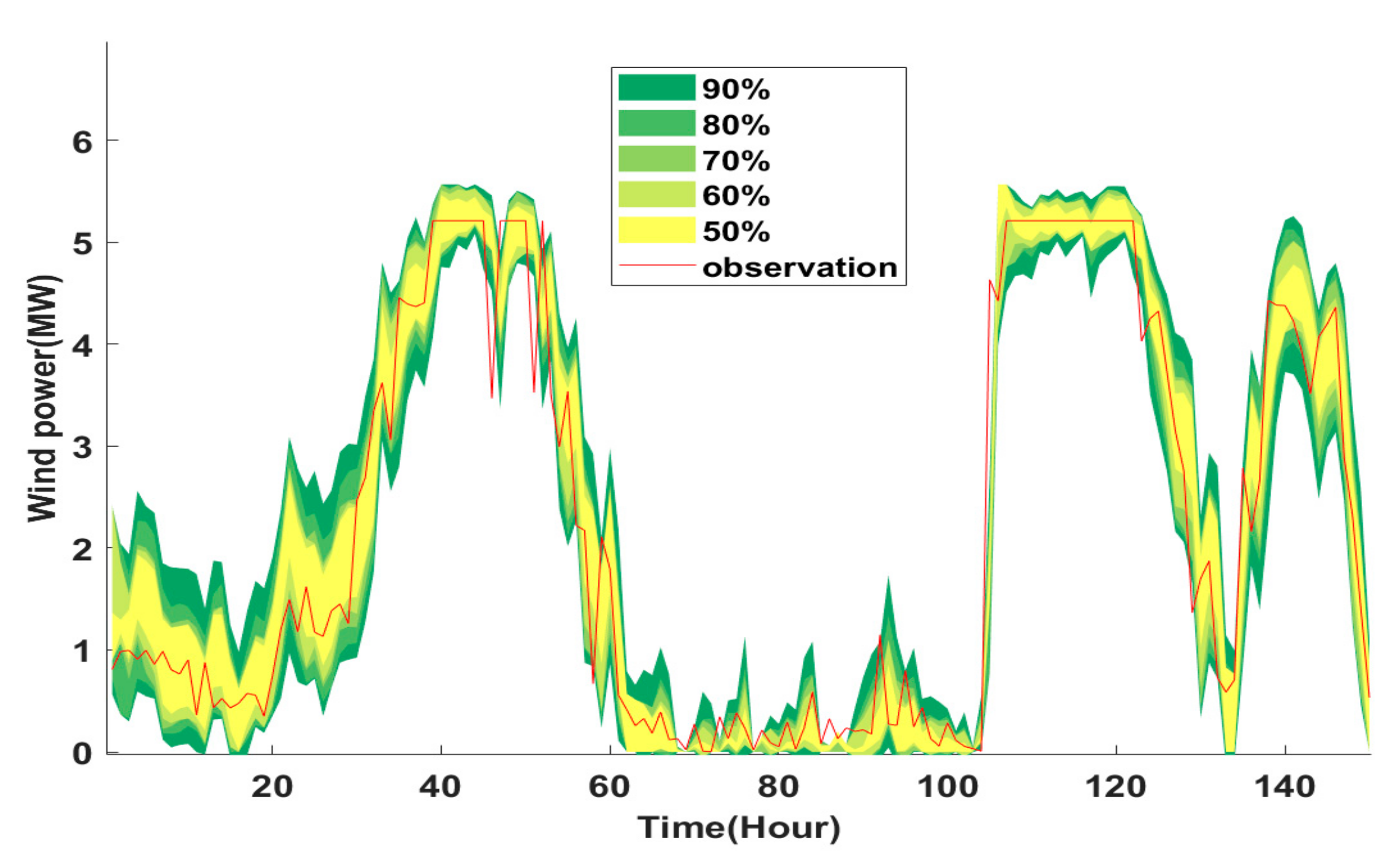
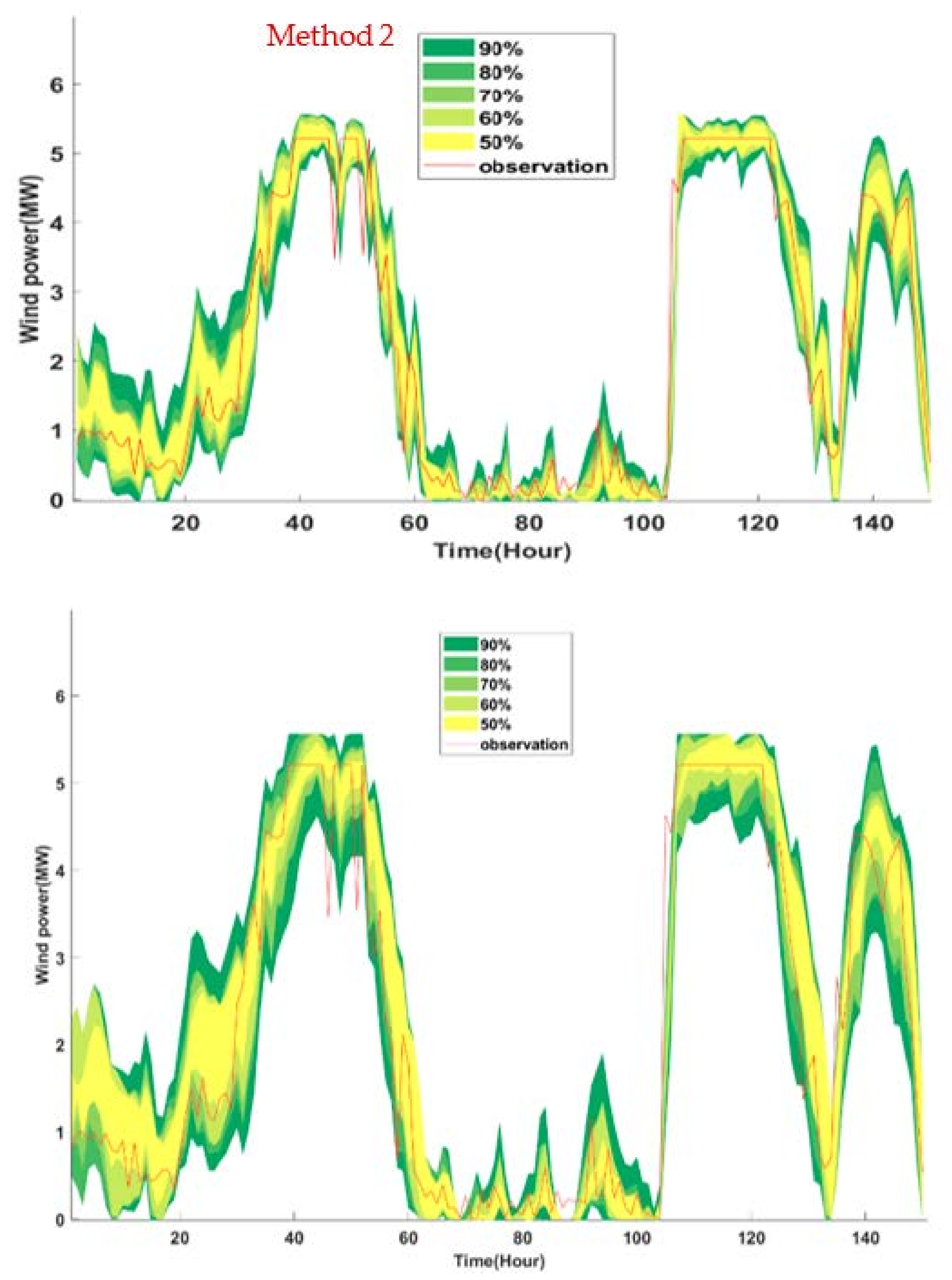
Figure 12, Figure 13 and Figure 14 present the results of probabilistic forecasting for the Hu-Si wind farm in the prediction intervals from 50 to 90% considering different NWP models as Method 1. Figure 15 and Figure 16 display the comparison of wind power forecasts by the proposed model with Method 2 and Method 3, respectively. To examine the accuracy of PIs (PI validity) and demonstrate the efficiency of the proposed method (method performance), Table 3, Table 4, Table 5, Table 6 and Table 7 summarize the values of PICP, PINAW, and CWC, respectively.
8. Discussions
The forecasting results can be compared in terms of forecasting validity, performance, and stability. Typically, PICPs represents the characteristics of reliability (PI validity), while PINAWs and CWCs represent the performance of forecasting methods (Accuracy).
In terms of PI validity, when PICP is greater than the related confidence level, PIs are theoretically valid. Otherwise, PI values are questionable. Table 3 shows that the PIs using the proposed method satisfy this requirement. Table 5 (Method 1b) and Table 6 (Method 2) also demonstrate that the PIs are valid. However, some of the PICPs that are obtained using Method 1a and Method 3 are smaller than the related confidence level, revealing that the selected input is not appropriate. Based on the results in Table 7 (Method 3), it is important to use a better dimension reduction technique or another powerful training model such as machine learning or deep learning.
In terms of forecasting performance, Table 3 reveals that the average of CWCs obtained by the proposed method is the smallest. Therefore, the proposed method has the highest forecasting performance with the preprocessing technique based on autoencoders and wind power curve calibration, which is followed by Method 1b and Method 2 shown in Table 5 and Table 6.
In terms of forecasting stability, by the proposed method, the mean of CWCs is always smaller than that using other methods (Methods 1a,b, 2, and 3). Additionally, the CWCs using Method 1a and Method 3 are large at some confidence levels because the obtained PICPs cannot reach up to the corresponding confidence levels, indicating that the forecasting stability by these models is low.
Based on the forecasting results, the PIs obtained by the proposed method are more efficient and insightful for decision-making than other methods.
9. Conclusions
Wind power forecasting plays a vital role in dealing with the intermittency and uncertainty characteristics of wind. Power system operations require a high accuracy forecasting model, since probabilistic wind power forecasts and NWP calibrations are still very challengeable. In this paper, a hybrid model has been proposed for three-hour-ahead wind power forecasting, which includes a dimensional reduction using autoencoders in the preprocessing step, the XGBoost training model for deterministic forecasting, and the consideration of different NWP models such as WRFD, RWRF, and WEPS. For evaluating the developed method, actual measured data from the Hu-Si wind farm located on Penghu island, Taiwan have been used for testing, and RMSE, PICP, PINAW, and CWC have been applied to identify the model performance.
This study demonstrates that the use of the machine learning model for training as well as the deep learning model for preprocessing input data is very important to improve forecasting performance. In addition, different NWP models should be considered in the forecasting module. Finally, the forecasting results herein in both deterministic and probabilistic forecasts show that the proposed model has better accuracy, stability, and reliability than other methods for short-term wind power forecasting.
Author Contributions
Conceptualization, Q.T.P. and Y.K.W., methodology, software, Q.T.P., validation, Y.K.W. and Q.D.P., formal analysis and investigation, Q.T.P. and Y.K.W., writing—original draft preparation, Q.T.P., writing—review and editing, Y.K.W. All authors have read and agreed to the published version of the manuscript.
Funding
This work is financially supported by the Ministry of Science and Technology (MOST) of Taiwan under Grant MOST 108-3116-F-194-001-. Project title: Development of Renewable Power Forecasting Technique Combing Numerical Weather Prediction and Artificial Intelligence.
Conflicts of Interest
The authors declare no conflict of interest.
References
- Wu, Y.-K.; Lee, T.-C.; Chang, S.-M.; Hsieh, T.-Y.; Chang, L.-T. Integration of large-scale renewable power into the Taiwan power system. In Proceedings of the 10th International Conference on Advances in Power System Control, Operation & Management (APSCOM 2015), Hong Kong, China, 8–12 November 2015; pp. 1–6. [Google Scholar]
- Xiaosong, H.; Zou, Y.; Yang, Y. Greener plug-in hybrid electric vehicles incorporating renewable energy and rapid system optimization. Energy 2016, 111, 971–980. [Google Scholar] [CrossRef]
- Ahmed, A.; Khalid, M. A review on the selected applications of forecasting models in renewable power systems. Renew. Sustain. Energy Rev. 2019, 100, 9–21. [Google Scholar] [CrossRef]
- Pinson, P.; Kariniotakis, G.; Nielsen, H.; Nielsen, T.; Madsen, H. Properties of Quantile and Interval Forecasts of Wind Generation and Their Evaluation. In Proceedings of the European Wind Energy Conference & Exhibition, Athens, Greece, 27 February–2 March 2006. [Google Scholar]
- Wu, Y.-K.; Su, P.-E.; Wu, T.-Y.; Hong, J.-S.; Hassan, M.Y. Probabilistic Wind-Power Forecasting Using Weather Ensemble Models. IEEE Trans. Ind. Appl. 2018, 54, 5609–5620. [Google Scholar] [CrossRef]
- Kavousi-Fard, A.; Khosravi, A.; Nahavandi, S. A New Fuzzy-Based Combined Prediction Interval for Wind Power Forecasting. IEEE Trans. Power Syst. 2016, 31, 18–26. [Google Scholar] [CrossRef]
- Zhang, G.; Wu, Y.; Wong, K.P.; Xu, Z.; Dong, Z.; Iu, H.H.-C. An Advanced Approach for Construction of Optimal Wind Power Prediction Intervals. IEEE Trans. Power Syst. 2014, 30, 2706–2715. [Google Scholar] [CrossRef]
- Kanna, B.; Singh, S. AWNN-Assisted Wind Power Forecasting Using Feed-Forward Neural Network. IEEE Trans. Sustain. Energy 2012, 3, 306–315. [Google Scholar]
- Sideratos, G.; Hatziargyriou, N. An Advanced Statistical Method for Wind Power Forecasting. IEEE Trans. Power Syst. 2007, 22, 258–265. [Google Scholar] [CrossRef]
- Wu, Y.-K.; Su, P.-E.; Hong, J.-S. An overview of wind power probabilistic forecasts. In Proceedings of the 2016 IEEE PES Asia-Pacific Power and Energy Engineering Conference (APPEEC), Xi’an, China, 25–28 October 2016; pp. 429–433. [Google Scholar]
- Bremen, L. Combination of Deterministic and Probabilistic Meteorological Models to enhance Wind Farm Power Forecasts. J. Phys. Conf. Ser. 2007, 75, 012050. [Google Scholar] [CrossRef]
- Qu, G.; Mei, J.; He, D. Short-term wind power forecasting based on numerical weather prediction adjustment. In Proceedings of the 2013 11th IEEE International Conference on Industrial Informatics (INDIN), Bochum, Germany, 29–31 July 2013; pp. 453–457. [Google Scholar]
- Xu, Q.; He, D.; Zhang, N.; Kang, C.; Xia, Q.; Bai, J.; Huang, J. A Short-Term Wind Power Forecasting Approach with Adjustment of Numerical Weather Prediction Input by Data Mining. IEEE Trans. Sustain. Energy 2015, 6, 1283–1291. [Google Scholar] [CrossRef]
- Xiong, Y.; Zha, X.; Qin, L.; Ouyang, T.; Xia, T. Research on wind power ramp events prediction based on strongly convective weather classification. IET Renew. Power Gener. 2017, 11, 1278–1285. [Google Scholar] [CrossRef]
- Wang, R.; Li, J.; Wang, J.; Gao, C. Research and Application of a Hybrid Wind Energy Forecasting System Based on Data Processing and an Optimized Extreme Learning Machine. Energies 2018, 11, 1712. [Google Scholar] [CrossRef] [Green Version]
- Khosravi, A.; Nahavandi, S. Combined Nonparametric Prediction Intervals for Wind Power Generation. IEEE Trans. Sustain. Energy 2013, 4, 849–856. [Google Scholar] [CrossRef]
- Wan, C.; Xu, Z.; Pinson, P.; Dong, Z.; Wong, K.P. Optimal Prediction Intervals of Wind Power Generation. IEEE Trans. Power Syst. 2014, 29, 1166–1174. [Google Scholar] [CrossRef] [Green Version]
- Quan, H.; Srinivasan, D.; Khosravi, A. Short-Term Load and Wind Power Forecasting Using Neural Network-Based Prediction Intervals. IEEE Trans. Neural Netw. Learn. Syst. 2013, 25, 303–315. [Google Scholar] [CrossRef] [PubMed]
- Wu, Y.-K.; Hong, J.-S. A literature review of wind forecasting technology in the world. In Proceedings of the 2007 IEEE Lausanne Power Tech, Lausanne, Switzerland, 1–5 July 2007; pp. 504–509. [Google Scholar]
- Dong, L.; Wang, L.; Khahro, S.F.; Gao, S.; Liao, X. Wind power day-ahead prediction with cluster analysis of NWP. Renew. Sustain. Energy Rev. 2016, 60, 1206–1212. [Google Scholar] [CrossRef]
- Wu, Y.-K.; Wu, Y.-C.; Hong, J.-S.; Phan, L.H.; Quoc, D.P. Probabilistic Forecast of Wind Power Generation with Data Processing and Numerical Weather Predictions. In Proceedings of the 2020 IEEE/IAS 56th Industrial and Commercial Power Systems Technical Conference (I&CPS), Las Vegas, NV, USA, 27–30 April 2020; pp. 1–11. [Google Scholar]
- Li, G.; Shi, J.; Zhou, J. Bayesian adaptive combination of short-term wind speed forecasts from neural network models. Renew. Energy 2011, 36, 352–359. [Google Scholar] [CrossRef]
- Breiman, L.; Friedman, J.H.; Olshen, R.A.; Stone, C.J. Classification and Regression Trees; CRC Press: Boca Raton, FL, USA, 2017. [Google Scholar]
- Lecun, Y. Modeles Connexionnistes de l’Apprentissage (Connectionist Learning Models). Ph.D. Thesis, Université Pierre et Marie Curie, Paris, France, 1987. [Google Scholar]
- Bourlard, H.; Kamp, Y. Auto-association by multilayer perceptrons and singular value decomposition. Biol. Cybern. 1988, 59, 291–294. [Google Scholar] [CrossRef] [PubMed]
- Hinton, G.E.; Zemel, R. Autoencoders, Minimum Description Length and Helmholtz Free Energy. In Advances in Neural Information Processing Systems; Cowan, J., Tesauro, G., Alspector, J., Eds.; Morgan-Kaufmann: Burlington, MA, USA, 1994; pp. 3–10. [Google Scholar]
- Li, Y.; Chen, X.; Li, C.; Tang, G.; Gan, Z.; An, X. A Hybrid Deep Interval Prediction Model for Wind Speed Forecasting. IEEE Access 2021, 9, 7323–7335. [Google Scholar] [CrossRef]
Figure 1.
Schematic diagram of probabilistic approaches based on deterministic Numerical Weather Prediction (NWP).
Figure 1.
Schematic diagram of probabilistic approaches based on deterministic Numerical Weather Prediction (NWP).

Figure 2.
Schematic diagram of probabilistic approaches based on ensemble NWPs.

Figure 3.
Schematic structure of an autoencoder with three fully connected hidden layers.

Figure 4.
Example of a 20-WEPS member of ensemble wind speeds. WEPS: Weather Research and Forecasting (WRF) ensemble prediction system.
Figure 4.
Example of a 20-WEPS member of ensemble wind speeds. WEPS: Weather Research and Forecasting (WRF) ensemble prediction system.

Figure 5.
Construction of an autoencoder for preprocessing ensemble wind speeds.

Figure 6.
Results of data preprocessing using WEPS ensemble members.

Figure 7.
Block diagram of the proposed probabilistic forecasting.

Figure 8.
Flow chart of probabilistic forecasting.

Figure 9.
Proposed three-hour-ahead deterministic forecasting model.

Figure 10.
Proposed three-hour-ahead probabilistic forecasting model.

Figure 11.
Testing sample of three-hour-ahead by the proposed model.

Figure 12.
Three-h-ahead probabilistic forecasting results by proposed method. WRFD, deterministic WRF; RWRF, radar WRF; WEPS.
Figure 12.
Three-h-ahead probabilistic forecasting results by proposed method. WRFD, deterministic WRF; RWRF, radar WRF; WEPS.

Figure 13.
Three-h-ahead probabilistic forecasting results by Method 1a (RWRF, WEPS).

Figure 14.
Three-h-ahead probabilistic forecasting results by Method 1b (WRFD, WEPS).

Figure 15.
Comparison of wind power forecasting results by the proposed method and Method 2.

Figure 16.
Comparison of wind power forecasting results by the proposed method and Method 3.


Table 1.
Input data description.
| Used Data | Input Data | Time |
|---|---|---|
| Historical data from wind farm | Wind Power (W) | Every hour from 7/2019 to 3/2020 |
| Data from NWPs | RWRF (m/s) WRFD (m/s) WEPS ensemble wind speed (m/s) | Every hour from 7/2019 to 3/2020 Every 3 h from 7/2019 to 3/2020 |
Table 2.
Important default values and tuned parameter settings of the proposed model.
| Parameter | Default | Proposed Model |
|---|---|---|
| Min_child_weight | 1 | 10 |
| Max_depth | 6 | 20 |
| Subsample | 1 | 0.8 |
| Lamda | 1 | 0.7 |
Table 3.
Three-hour-ahead Predicted Intervals (PIs) using the proposed model that considers WRFD, RWRF, and WEPS.
Table 3.
Three-hour-ahead Predicted Intervals (PIs) using the proposed model that considers WRFD, RWRF, and WEPS.
| Confidence Level (%) | PICP | PINAW | CWC |
|---|---|---|---|
| 50 | 52.55 | 7.68 | 7.68 |
| 60 | 63.26 | 10.41 | 10.41 |
| 70 | 76.53 | 12.94 | 12.94 |
| 80 | 83.16 | 16.71 | 16.71 |
| 90 | 90.82 | 20.95 | 20.95 |
Table 4.
Three-hour-ahead PIs using RWRF and WEPS (Method 1a).
| Confidence Level (%) | PICP | PINAW | CWC |
|---|---|---|---|
| 50 | 48.93 | 8.90 | 19.38 |
| 60 | 64.08 | 12.75 | 12.75 |
| 70 | 72.88 | 16.33 | 16.33 |
| 80 | 80.70 | 19.80 | 19.80 |
| 90 | 89.00 | 24.40 | 90.30 |
Table 5.
Three-hour-ahead PIs using WRFD and WEPS (Method 1b).
| Confidence Level (%) | PICP | PINAW | CWC |
|---|---|---|---|
| 50 | 58.08 | 8.90 | 8.90 |
| 60 | 74.74 | 13.09 | 13.09 |
| 70 | 80.30 | 15.63 | 15.63 |
| 80 | 82.32 | 18.86 | 18.86 |
| 90 | 90.90 | 24.05 | 24.05 |
Table 6.
Three-hour-ahead PIs using Method 2.
| Confidence Level (%) | PICP | PINAW | CWC |
|---|---|---|---|
| 50 | 54.55 | 9.43 | 9.43 |
| 60 | 66.07 | 13.30 | 13.30 |
| 70 | 71.43 | 15.88 | 15.88 |
| 80 | 80.30 | 19.59 | 19.59 |
| 90 | 92.07 | 22.07 | 22.07 |
Table 7.
Three-hour-ahead PIs using Method 3.
| Confidence Level (%) | PICP | PINAW | CWC |
|---|---|---|---|
| 50 | 46.50 | 9.02 | 46.50 |
| 60 | 66.69 | 12.84 | 12.84 |
| 70 | 75.17 | 15.99 | 15.99 |
| 80 | 80.80 | 18.17 | 18.17 |
| 90 | 86.82 | 22.43 | 490.20 |
Publisher’s Note: MDPI stays neutral with regard to jurisdictional claims in published maps and institutional affiliations. |
© 2021 by the authors. Licensee MDPI, Basel, Switzerland. This article is an open access article distributed under the terms and conditions of the Creative Commons Attribution (CC BY) license (http://creativecommons.org/licenses/by/4.0/).
Share and Cite
MDPI and ACS Style
Phan, Q.T.; Wu, Y.K.; Phan, Q.D. A Hybrid Wind Power Forecasting Model with XGBoost, Data Preprocessing Considering Different NWPs. Appl. Sci. 2021, 11, 1100. https://0-doi-org.brum.beds.ac.uk/10.3390/app11031100
AMA Style
Phan QT, Wu YK, Phan QD. A Hybrid Wind Power Forecasting Model with XGBoost, Data Preprocessing Considering Different NWPs. Applied Sciences. 2021; 11(3):1100. https://0-doi-org.brum.beds.ac.uk/10.3390/app11031100
Chicago/Turabian StylePhan, Quoc Thang, Yuan Kang Wu, and Quoc Dung Phan. 2021. "A Hybrid Wind Power Forecasting Model with XGBoost, Data Preprocessing Considering Different NWPs" Applied Sciences 11, no. 3: 1100. https://0-doi-org.brum.beds.ac.uk/10.3390/app11031100
Note that from the first issue of 2016, this journal uses article numbers instead of page numbers. See further details here.