Advances in High-Precision NO₂ Measurement by Quantum Cascade Laser Absorption Spectroscopy

Abstract

Nitrogen dioxide (NO${}_2$) is a major tropospheric air pollutant. Its concentration in the atmosphere is most frequently monitored indirectly by chemiluminescence detection or using direct light absorption in the visible range. Both techniques are subject to known biases from other trace gases (including water vapor), making accurate measurements at low concentration very challenging. Selective measurements of NO${}_2$ in the mid-infrared have been proposed as a promising alternative, but field deployments and comparisons with established techniques remain sparse. Here, we describe the development and validation of a quantum cascade laser-based spectrometer (QCLAS). It relies on a custom-made astigmatic multipass absorption cell and a recently developed low heat dissipation laser driving and a FPGA based data acquisition approach. We demonstrate a sub-pptv precision (1 $\sigma$) for NO${}_2$ after 150 s integration time. The instrument performance in terms of long-term stability, linearity and field operation capability was assessed in the laboratory and during a two-week inter-comparison campaign at a suburban air pollution monitoring station. Four NO${}_2$ instruments corresponding to three different detection techniques (chemiluminescence detection (CLD), cavity-attenuated phase shift (CAPS) spectroscopy and QCLAS) were deployed after calibrating them with three different referencing methods: gas-phase titration of NO, dynamic high-concentration cylinder dilution and permeation. These measurements show that QCLAS is an attractive alternative for high-precision NO${}_2$ monitoring. Used in dual-laser configuration, its capabilities can be extended to NO, thus allowing for unambiguous quantification of nitrogen oxides (NO${}_x$), which are of key importance in air quality assessments.

1. Introduction

Nitrogen dioxide (NO${}_2$) is an important atmospheric gas-phase pollutant because of its role in O${}_3$ formation [1,2] and its influence on the oxidation capacity of the atmosphere, e.g., by reaction with the hydroxyl radical (OH) and formation of the nitrate radical (NO${}_3$) [3,4]. It also has a direct impact on human health and on the biosphere [5,6,7,8,9]. Furthermore, the oxidation products of NO${}_2$ strongly influence the chemistry of the atmosphere, e.g., oxidation capacity, aerosol particles formation/aging, long-range pollutants transport and nitrates deposition [10,11,12,13,14]. The amount fraction of NO${}_2$ in tropospheric air can rise up to many tens of part-per-billion by volume (ppbv, equivalent to nmol/mol) in densely populated and industrial areas, while, in the free troposphere, its level is usually in the part-per-trillion by volume (pptv, equivalent to pmol/mol) range. The Global Atmospheric Watch program (GAW) of the World Meteorological Organization (WMO) has defined guidelines in terms of ambient NO${}_2$ measurement precision and uncertainties in order to establish an optimal monitoring [15]. These guidelines state that the instrumental limit of detection (LOD) in remote environments, i.e., very weakly impacted by anthropogenic activities, should be as low as 5 pptv (3 $\sigma$) with an uncertainty below 5%.

There is only a very limited number of instruments capable of reaching such a high precision in field conditions. The most widely used techniques for in-situ measurement of trace amounts of NO${}_2$ are based on indirect detection by chemiluminescence (CLD) or on direct detection by laser absorption spectroscopy (LAS) in the visible range (VIS). The CLD technique relies on the reduction of NO${}_2$ to nitric oxide (NO) using a molybdenum or a photolytic converter [16,17]. This reaction is followed by the detection of NO by using O${}_3$ as a reactant to form excited NO${}_2$, which deactivates by light emission (chemiluminescence). This method has several drawbacks, including interferences from other nitrogen oxides present in the atmosphere that release NO${}_2$ (positive bias) during the reduction process [18,19] and quenching of the excited NO${}_2$ by water (negative bias) [20]. The precision of the CLD technique is limited by the fact that the detected luminescence signal observed after the NO${}_2$ conversion accounts for the sum of ambient NO plus NO${}_2$ (NO${}_x$). This requires subtracting the ambient NO concentration (obtained by bypassing the NO${}_2$ converter) from the total measured NO${}_x$ to obtain the NO${}_2$ concentration, thus decreasing the precision of the NO${}_2$ measurements. Nevertheless, LODs between 3 and 15 pptv have been reported [21,22]. Among the techniques using laser absorption in the visible range, the most established ones are based on cavity enhanced spectroscopy (CES), such as cavity ring down spectroscopy (CRDS) or cavity attenuated phase shift (CAPS) spectroscopy [23,24,25,26]. While these methods offer in general a similar LOD than the CLD technique, they are still subject to interferences from water due to Rayleigh scattering effects [27,28,29] and potentially from dicarbonyl compounds (mostly glyoxal and methylglyoxal) by light absorption [27]. To avoid post-corrections on ambient air measurements in humid conditions, modern commercial instruments often include driers in their inlets. This approach, however, still requires applying a correction for the artificial increase in the NO${}_2$ signal due to the removal of water from the sample. Furthermore, long-term measurements might suffer from changes in the drier efficiency and in its reactivity toward NO${}_2$.

In parallel to the development of spectroscopic techniques in the visible range, mid-infrared (MIR) detection of NO${}_2$ has also been demonstrated using lead-salt tunable diode laser absorption spectroscopy (TDLAS) [30,31], and then further developed using quantum cascade laser absorption spectroscopy (QCLAS) [32]. Currently, these techniques allow reaching a very high precision, especially in combination with astigmatic multipass absorption cells. LODs below 10 pptv using QCLAS have been achieved with very long optical path length of 200 m [33,34]. The CLD, CES and TDLAS techniques have been widely used and their performance investigated in a significant number of laboratory studies and inter-comparison experiments [21,31,35,36]. In contrast, reviews of QCLAS for high-precision NO${}_2$ detection are sparse, despite its demonstrated high sensitivity and selectivity [32].

Existing uncertainties related to measurements and calibration methods for direct ambient NO${}_2$ measurements is the rational for the recent MetNO2 project of the European Metrology Programme for Innovation and Research (EMPIR), funded by the European Association of National Metrology Institutes (EURAMET). More accurate measurements of NO${}_2$ will bring greater confidence in identified trends in air quality and support the development and implementation of effective, evidence-based mitigation policies needed to reduce pollution levels. Within this context, the following paper provides details on the development, characterization and validation of a new QCLAS instrument, including the analysis of a two-week field inter-comparison at the suburban site Dübendorf (Switzerland).

2. Materials and Methods

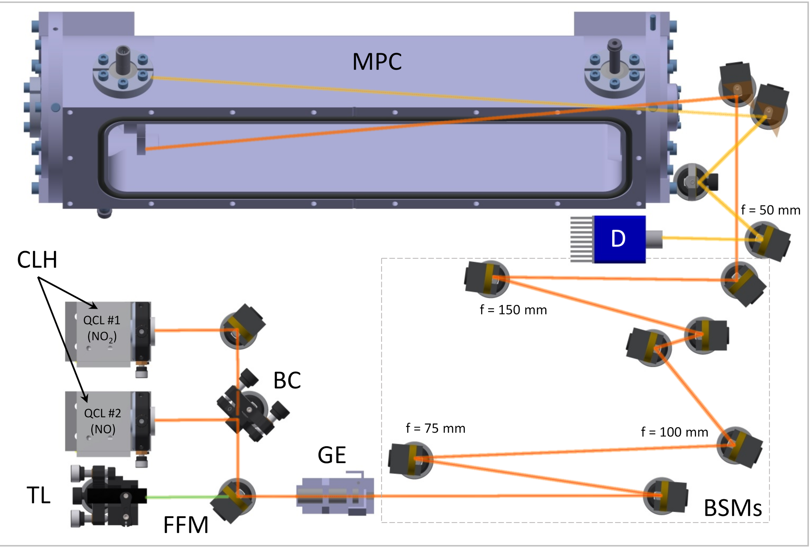
2.1. Description of the Dual-Laser Spectrometer

The main target of our instrumental design and development was to reach high precision NO${}_2$ measurements under field conditions with possible extension towards other relevant species, such as NO. The chemistry of these compounds in the atmosphere is strongly interconnected since they share common anthropogenic sources and are involved in rapid cyclic processes. From an air quality perspective, especially for urban or near-road environments, the sum of both is often considered and referred to as NO${}_x$. Considering these aspects, a dual-laser concept has been implemented [32,37], where two distributed feedback quantum cascade lasers (DFB-QCLs, Alpes Laser SA, St-Blaise, Switzerland) with distinct emission frequencies are combined and coupled into an astigmatic multipass absorption cell (MPC). For completeness, the instrumental setup is described for both lasers. However, since NO${}_2$ is the target substance of the present study, only the results that are relevant for NO${}_2$ are shown. The first laser emits in the spectral range around 1600 cm${}^{-1}$, corresponding to the ${\nu }_3$ ro-vibrational band of NO${}_2$. Similar to previous studies [32,34], the doublet NO${}_2$ line at 1599.9 cm${}^{-1}$ is used for concentration retrieval. This doublet-line was chosen for its intensity and because it is well separated from any neighboring water lines (see below). The second laser emits in the 1900 cm${}^{-1}$ range, and NO concentration are derived using a doublet line at 1900.1 cm${}^{-1}$.

Both lasers are driven in intermittent continuous-wave mode (iCW). This driving approach and its advantages have been described elsewhere [38,39,40]. Briefly, the laser driver rapidly turns on and off the current to the lasers, which results in an emission frequency sweep of the DFB-QCL due to the change in the refractive index of the laser device induced by Joule heating. This driving mode has the advantage of lower heat dissipation requirements and thus more compact thermal management solutions compared to the conventional continuous-wave (CW) mode. For NO${}_2$ and NO, the laser drivers apply current to the lasers for 45 and 30 s, resulting in emission frequency sweeps over 0.8 and 0.4 cm${}^{-1}$, respectively. The laser current drivers are triggered by a field-programmable gate array (FPGA) embedded on a commercial system-on-chip (Alpha250, Koheron, Lorient, France). This board features a dual-core ARM processor and a fast analog front-end with dual-channel 14-bit ADCs and 16-bit DACs of 100 MHz bandwidth, and it is coupled to a custom-made extension board. The FPGA firmware (VHDL-Code) and the Linux service routines (C-Code) were custom developed to support the functionalities required for the spectroscopic setup. For higher flexibility in data acquisition, several user-defined time-windows within a spectral scan are supported. The summation of consecutive spectra is implemented in real-time with digital signal processors (DSP) and dual port block random access memory (BRAM). The averaged spectra are then sent to an external computer via a TCP/IP-interface for spectral analysis. Further functionalities to control peripherals, such as laser temperature controllers, sample pressure and temperature sensors, valve switching, etalon-flip, etc. are handled by the custom extension PCB containing additional high-precision ADC, DAC and DIO ports. These functionalities were implemented using the Inter-Integrated Circuit (I2C) communication protocol.

The overall instrument is composed of two main units. One module (80 × 60 × 40 cm) contains the optical setup (Figure 1), while the other compartment (45 × 40 × 20 cm) houses the electronic hardware (data acquisition (DAQ) unit, power supplies, embedded computer, temperature controllers and laser drivers). A thermo-chiller (T-Three, Solid State Cooling System, Wappingers Falls, NY, USA) is used to stabilize the temperature of the water-cooled elements mounted in series (laser housings, optical board, lasers current drivers and thermoelectric (TEC) controllers). The DFB-QCLs are mounted in a custom-made compact laser housing (CLH) with embedded TEC element. A few millimeters after the CLH, an AR coated aspheric lens (Black Diamond-2, Thorlabs Inc., Newton, NJ, USA) is placed to collimate the output laser beam. This external collimation solution was chosen to allow more flexibility in the beam shaping. Afterwards, the two laser beams are combined by a custom-made IR/IR beam combiner (LohnStar Optics Inc., Escondido, CA, USA) and directed onto a series of plane and spherical, gold-coated mirrors used to further steer and shape the combined IR beams to appropriately fulfill the coupling and beam matching conditions of the MPC (see, e.g., [41]). After multiple reflections, the IR beam exits the MPC and is aimed at a MIR detector (PVI-4TE-6, VIGO System, Ożarów Mazowiecki, Poland) with a high-bandwidth pre-amplifier (PIP-DC-200M).

The concentrations of NO and NO${}_2$ are retrieved by fitting a Voigt function to the measured spectra using the Levenberg–Marquardt least-squares algorithm implemented in LabView (National Instruments Inc., Austin, TX, USA). The transmission spectrum background (baseline) is fitted using a polynomial function. The spectral line intensity and the pressure broadening coefficients are taken from the HITRAN2016 database [42], whereas the sample pressure and temperature are measured and taken into account in the fitting procedure. An example of a transmission spectrum for NO${}_2$ with the associated fitted curves using Voigt profiles are shown in Figure 2. To convert the time scale into frequency scale, a two inch long solid germanium etalon with a free spectral range (FSR) of 0.0243 cm${}^{-1}$ can be placed in the beam path.

For the highest stability, but especially when measuring at very low NO${}_2$ concentration levels (<0.1 ppbv), where the detector noise and optical fringes dominate the NO${}_2$ absorption signal, a frequency locking mechanism is implemented using a neighboring water absorption line at 1600.25 cm${}^{-1}$ (Figure 2). For this, the retrieved central position of this water absorption line is used as a reference for determining the position of the NO${}_2$ line, assuming a constant frequency separation between both as given in the HITRAN database. Besides this passive frequency lock, we also implemented an active locking, where the water absorption line position is used as feedback signal to the laser TEC to adjust the heat-sink temperature such that this position remains constant ($\pm 1\times {10}^{-4}$ cm${}^{-1}$). For ambient air measurements, the water concentration is high enough to assure a good signal-to-noise ratio (SNR) so that its absorption line can always be used in both frequency locking mechanisms.

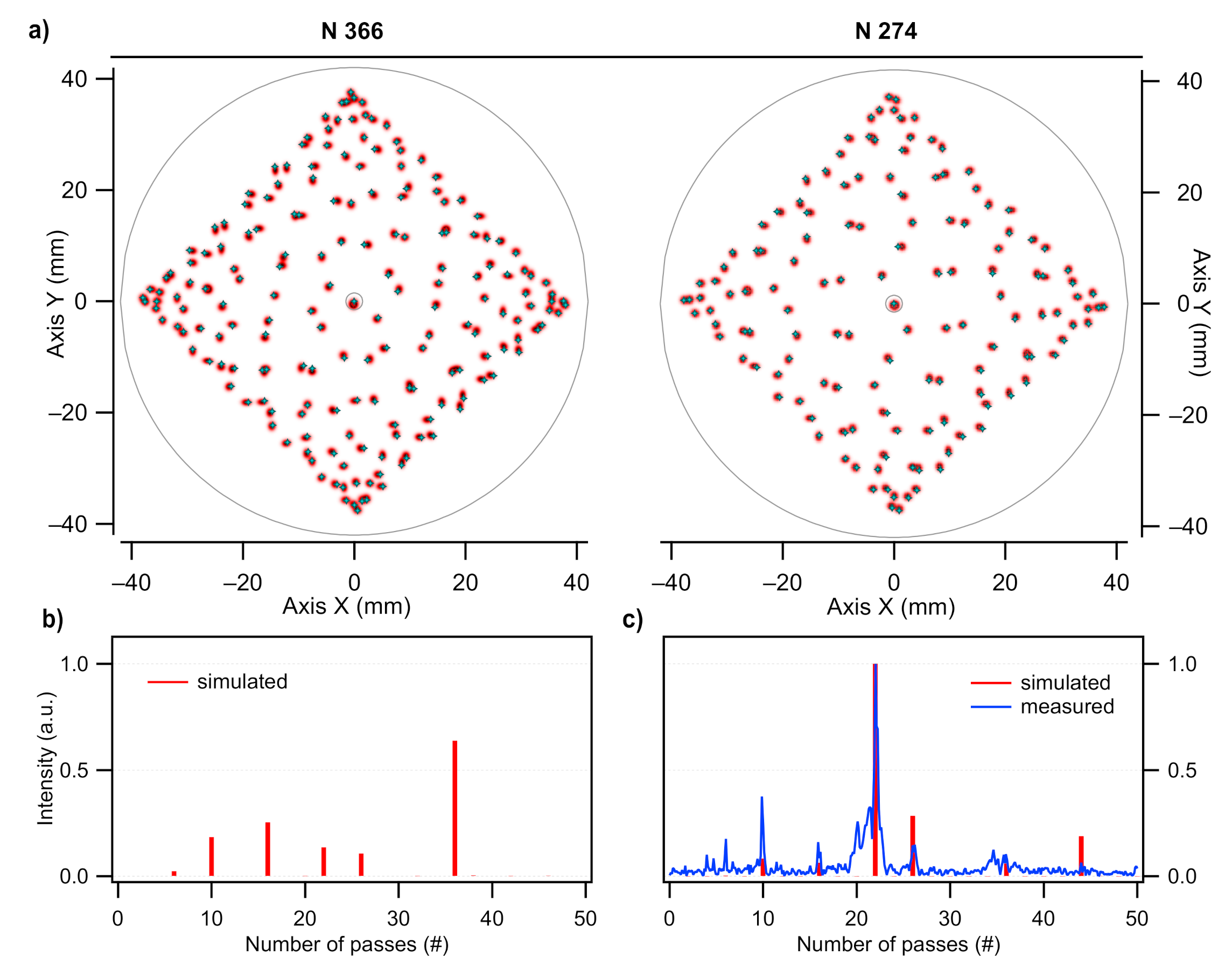
2.1.1. Instrument Inlet and Custom-Made Multipass Cell

The MPC has been developed with special focus on the specific properties of NO${}_2$, known for its reactivity toward surfaces, but also aiming for an optical path length (OPL) of at least 100 m and a high mechanical stability to achieve the targeted precision of a few pptv NO${}_2$. The MPC body is machined out of a single piece of electro-polished aluminum and closed by two high-vacuum KF-flanges and a top lid. All these parts are coated (SilcoNert©2000, SilcoTek, Bellefonte, PA, USA) to minimize surface losses of NO${}_2$. For the same reason, all the gas handling elements up to the MPC are either made out of polytetrafluorethylen (PTFE) or SilcoNert-coated, while the entire sampling line uses perfluoralkoxy (PFA) tubing. Right after the intake point, the air flows through a solenoid three-way valve (International Polymer Solutions, Irvine, CA, USA), used to switch between ambient and NO${}_x$-free air, followed by a PTFE membrane filter (TE38, Cytiva Europe GmbH, Freiburg, Germany; pore ∅ = 5.0 m). A coated stainless steel needle valve is placed immediately before the MPC to adjust the sample pressure in the range of 30–100 mbar. This low pressure regime improves the selectivity of the instrument by leading to narrower spectral line widths due to the reduced pressure broadening effect on the absorption lines. A diaphragm pump (KNF Neuberger GmbH, Freiburg, Germany) is used to maintain a constant flow of 0.8 L/min (at ambient pressure) through the system.

To optimize the optical performance of the MPC, an extensive investigation on the beam reflection pattern on the mirrors was performed. Previous work have shown that overlapping of neighboring reflection spots on the mirrors creates interference fringes on the measured transmission spectrum that may impact the precision and long-term stability of the measurements [37,43]. Therefore, two key aspects were considered, searching for patterns with: (i) the highest possible mutual distance between neighboring spots in general; and (ii) a special focus on the lowest possible overlap between spots separated by a low number of passes through the MPC. This latter case corresponds to fringes with a low FSR that more likely interfere with the measurements. Following the approach described by McManus et al. [37], a custom-made software was developed to survey all possible patterns and to identify those fulfilling the above mentioned requirements.

A reflection pattern is defined by four independent parameters: the mirrors distance (D), the radii of the astigmatic mirrors ($R_x$ and $R_y$) and the relative rotation angle between the two mirrors ($\tau$) around the optical axis. Within the full range of each of these parameters, a large number of patterns exist that fulfill the re-entrant condition, i.e., the beam exits the cell after a certain number of reflections (N). Limiting the range for $\tau$ (± 15${}^{{}^{\circ }}$) and the astigmatism (ratio $R_x$/$R_y$, 10%) for a given mirror distance (400 ± 5 mm) reduces the number of possible re-entrant patterns to a few hundred. The final choice among all these possibilities requires estimating the intensity and spectral positioning of interference fringes resulting from spots overlapping on the mirrors reflective surfaces.

Based on this survey, a pattern of 366 passes (abbreviated as N366) corresponding to an OPL of 146 m was selected (Figure 3). This pattern is obtained with a mirror spacing of 40 cm and twist of 5 ${}^{{}^{\circ }}$ for mirror radii of 610.0 and 676.6 mm. These parameters were calculated based on the paraxial approximation. Further validation by using 3D ray-tracing simulation (FRED, Photon Engineering, Tucson, AZ, USA) showed that a small adjustment of the mirror distance (in the order of 0.1 mm, i.e., 0.025% of the paraxial value) is necessary in order to perfectly fulfill the re-entrant condition under non-paraxial conditions. The patterns obtained with the ray-tracing simulation shown in Figure 3 correspond to the adjusted mirror distance. A mirror diameter of 80 mm was then chosen as a good compromise between spots spreading and MPC footprint and volume (≈ 3 L). Considering the pattern’s high number of passes, it has high demands on the mirror surface quality and reflectivity. Therefore, the astigmatic mirrors were custom-made by diamond-turning (LT Ultra-Precision Technology, Herdwangen-Schönach, Germany) of a NiP coated (100 m) aluminum substrate (RSA 6061). This assures the highest surface quality, which is then further homogenized by a post-polishing process, resulting in a surface roughness better than 2 nm $R_a$. Finally, a custom-made coating (LohnStar Optics, Escondido, CA, USA) was applied to enhance the reflectivity (R > 99.3%) for both the 1600 and 1900 cm${}^{-1}$ spectral ranges. First tests with this pattern showed that the power on the detector was too low, thus limiting the detection limit. Therefore, an alternative pattern with 274 reflections, using the same mirrors, was chosen, which proved to be a better compromise between optical SNR and final sensitivity (in terms of concentration). This pattern is shown in Figure 3 and corresponds to D = 39.7 cm and $\tau$ = 4 ${}^{{}^{\circ }}$. The calculated OPL with the N274 pattern is 109.02 m. This value was confirmed experimentally by measuring the time delay between the optical signal received by the detector when the laser beam is either passing or bypassing the MPC. This resulted in 109.1 ± 1.7 m (1 $\sigma$) which agrees well with the value obtained from the simulation.

The simulated interference fringes spectra for the N366 and N274 patterns are shown in Figure 3. Both spectra are normalized to the intensity of the 22 passes fringe of the N274 pattern to allow for comparison. A measured fringe spectrum for the N274 pattern is also shown in Figure 3. These data are obtained by applying a fast Fourier transform (FFT) to the normalized residual from a polynomial fit of the measured transmission spectrum of NO${}_x$-free synthetic air (Messer Schweiz AG, Lenzburg, Switzerland; abbreviated in the following text and figures as synthetic air). The measured spectra are normalized to the measured intensity of the strongest fringe, corresponding to 22 passes. The overall agreement between measurement and simulation for N274 is good in terms of both fringe position and relative intensity. The only exceptions are the fringes at four and six passes equivalent FSR in the measured spectrum, which may result from imperfect alignment. This comparison between measured and simulated spectra supports the simulation approach for estimating interference fringes intensity. The comparison between the N274 and N366 simulated spectra shows that, despite the higher number of passes of the latter one, its predicted fringe intensity is similar to or lower than for the N274 pattern. This indicates that a further improvement of the sensitivity would be possible by using a more powerful QCL and the N366 pattern.

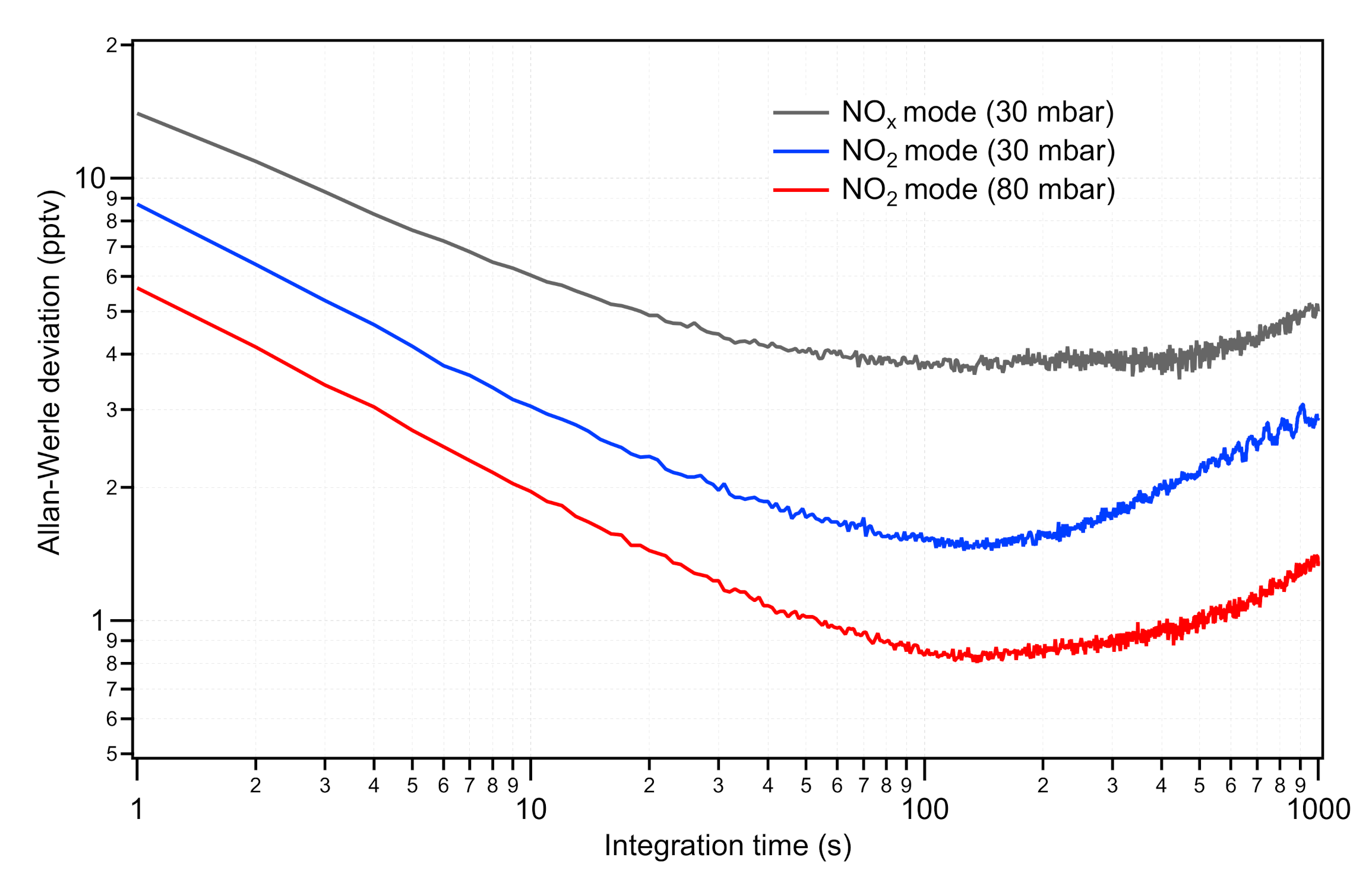
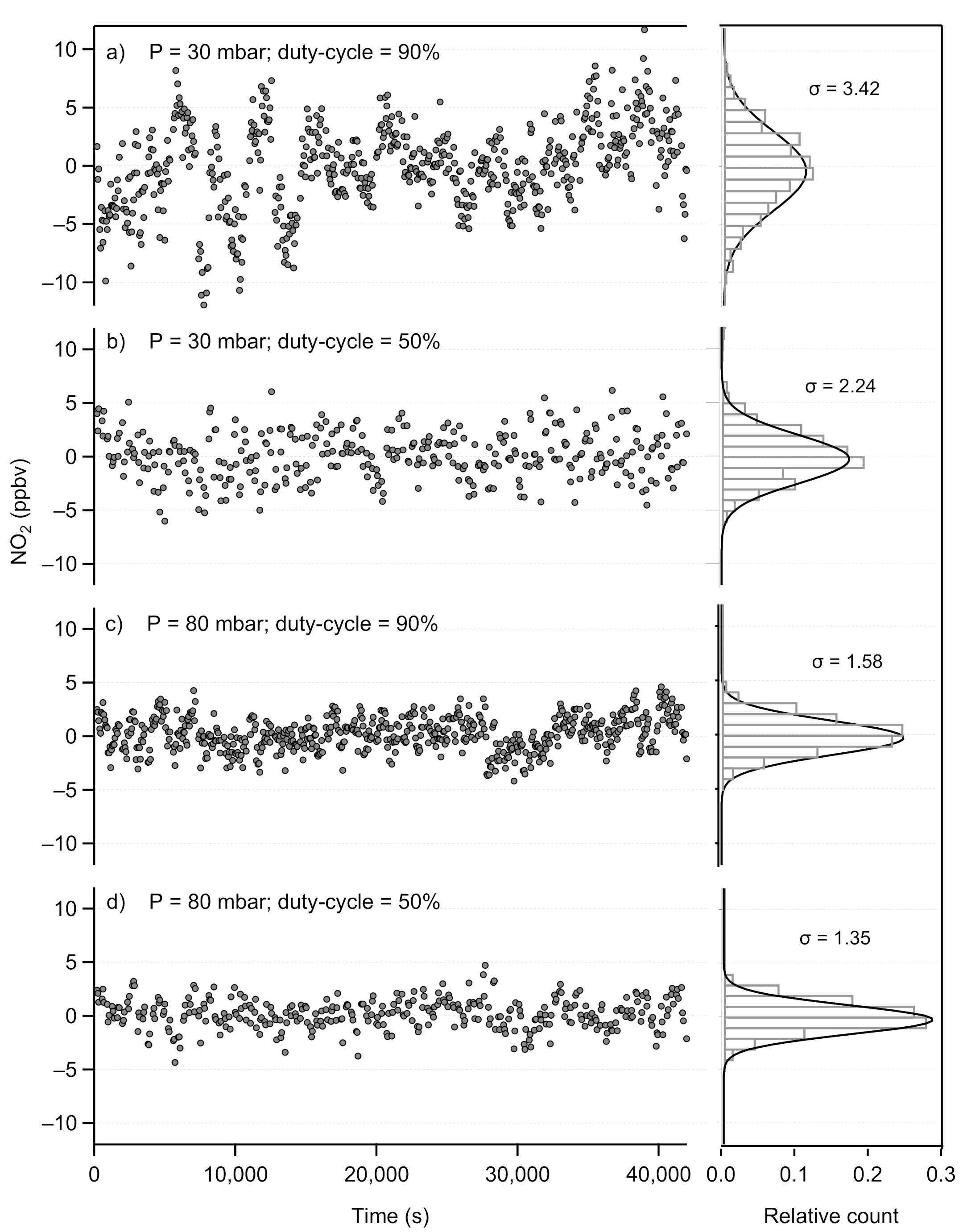
2.1.2. Performance Assessment

The measurement precision of our instrument for NO${}_2$ was estimated by using the Allan–Werle deviation technique [44]. For this, synthetic air was continuously measured over 12 h, and the NO${}_2$ line position was locked by using the passive frequency-locking method described above. The reference water line was obtained by artificially humidifying the air to about 200 ppmv H${}_2$O using humidified charcoal in the sampling line. Figure 4 summarizes measurements obtained under various operating conditions by showing the associated Allan–Werle deviation plot. Measurements at two different sample pressures (gas pressure in the MPC), namely 80 and 30 mbar, are presented as we found this parameter to have the most significant influence on the results especially in terms of water induced spectral interferences, as described in Section 2.1.3. In addition, two distinct operating modes are considered: (i) NO${}_x$ mode, corresponding to the detection of both NO and NO${}_2$ for which both lasers are emitting alternatively at a repetition rate of 10 kHz; and (ii) NO${}_2$ mode, corresponding to the detection of NO${}_2$ only, which allows a higher repetition rate (up to 15 kHz).

Within the examined measurement conditions, we found that the best short-term (1 s) precision (${\sigma }_{1s}$) for NO${}_2$ is achieved at 80 mbar sample pressure and operating in NO${}_2$ mode. In this case, the Allan–Werle deviation minimum (${\sigma }_{min}$) of 0.8 pptv is achieved after 150 s averaging time. At 30 mbar, the precision is about twice lower, which is simply due to the decrease in number density caused by the lower sample pressure. In NO${}_x$ operating mode, the precision decreases further, which is the result of lower repetition rate, i.e., fewer spectra are averaged within 1 s. Repeated measurements between 30 and 80 mbar in NO${}_2$ mode resulted in ${\sigma }_{1s}$ values consistently between 5 and 10 pptv and ${\sigma }_{min}$ values between 0.8 and 2 pptv with corresponding optimal averaging times between 100 and 300 s. A similar test for NO at 80 mbar in NO${}_x$ mode showed Allan–Werle deviation values of ${\sigma }_{1s}$ = 70 pptv and ${\sigma }_{min}$ = 20 pptv at 150 s integration time.

In summary, our custom-made instrument can reach, depending on the operating conditions, sub-pptv precision for NO${}_2$. This represents a factor 2–3 improvement compared to previous work on high-precision NO${}_2$ measurements by QCLAS, despite the short OPL of 110 m.

Table 1. Comparison of reported precision for NO${}_2$ measurements by QCLAS and TDLAS. OPL, optical path length; N, number of passes of the laser beam in the MPC; D, distance between the MPC mirrors; P, pressure in the MPC; ${\sigma }_{1s}$, Allan deviation at 1 s resolution; ${\sigma }_{min}$, minimum Allan deviation; time, integration time corresponding to ${\sigma }_{min}$.

Reference	OPL (m) / N / D (cm)	Lasers	P (mbar)	${\mathit{\sigma }}_{1\mathit{s}}$ (pptv)	${\mathit{\sigma }}_{\mathit{min}}$ (pptv) / Time (s)
[34]	204/434/47	dual	50	20	3/180
[33]	210/238/88	dual	53	10	1.7/60
[45]	153/174/88	dual	33	30	7/60
this work	110/274/40	single	80	5.5	0.8/150
this work	110/274/40	single	30	9	1.6/150
this work	110/274/40	dual	30	15	4/150

summarizes the results of this work in terms of Allan deviation and those found in the literature. It only includes studies about high-precision measurements with ${\sigma }_{min}$ <10 pptv.

Figure 4 also indicates that, after about 150 s, a drift starts to dominate the instrument’s precision. To prevent this drift in the ambient air NO${}_2$ measurements, synthetic air is periodically sampled during 1 min by switching the electronic three-way valve at the instrument’s inlet. Amount fractions of NO${}_2$ measured during these periods are linearly interpolated and then subtracted from the measurements, referred to as zero-drift correction. The response time (99%) of the instrument at 0.8 L/min is approximately 45 s, which results in a transition time of 3 min between the measurement periods to correct for zero drift (hereafter zeroing time). The frequency of this ”zeroing” defines the duty cycle which is obtained by dividing the measurement duration by the total cycle duration. For the measurements presented in Section 3 a duty cycle of 63% was used, corresponding to 5 min of measurement for 3 min of zeroing time.

Some experimental conditions require using higher duty cycles (longer measurement periods) to avoid dead-times (e.g., kinetic experiments, transient mixing ratios variations detection, etc.). To quantify the influence of this parameter on the instrument’s precision, we corrected the time-series used for obtaining the Allan–Werle plots (Figure 4) with the drift correction procedure describe above. Since these time-series were obtained by continuous sampling of synthetic air without any valve switching, the data are artificially categorized into measurement and zeroing data. Figure 5 presents the drift-corrected time-series measured in NO${}_2$ mode at 80 and 30 mbar with duty cycles of 50% and 90%, corresponding to 3 and 27 min of measurements and 3 min of zeroing time.

The associated histograms of the relative frequency count for each dataset is shown on the right. The least spread with a standard deviation (1 $\sigma$) of 1.35 pptv is obtained with the duty cycle of 50% at 80 mbar. With the same duty cycle but at 30 mbar, the standard deviation is 2.24 pptv. In each case, however, the precision is good enough for measurements at very low NOx conditions as found in the most remote locations. As mentioned above, the GAW program recommends a LOD (defined as three times the standard deviation) below 5 pptv for measuring in remote conditions. In our case, using a zero drift correction with a duty cycle of 50% yields LODs of 4.1 and 6.7 pptv (equivalent to $1.09\times {10}^8$ and $1.78\times {10}^8$ molecules/cm${}^3$ at standard temperature and pressure conditions, respectively) at 80 and 30 mbar, respectively, at 1 min resolution. Averaging the data over longer time periods helps improving the LOD. For example, working at a resolution of 12 min, which corresponds to two measurement cycles at a duty cycle of 50%, permits LODs of 3.0 and 3.9 pptv at 80 and 30 mbar, respectively.

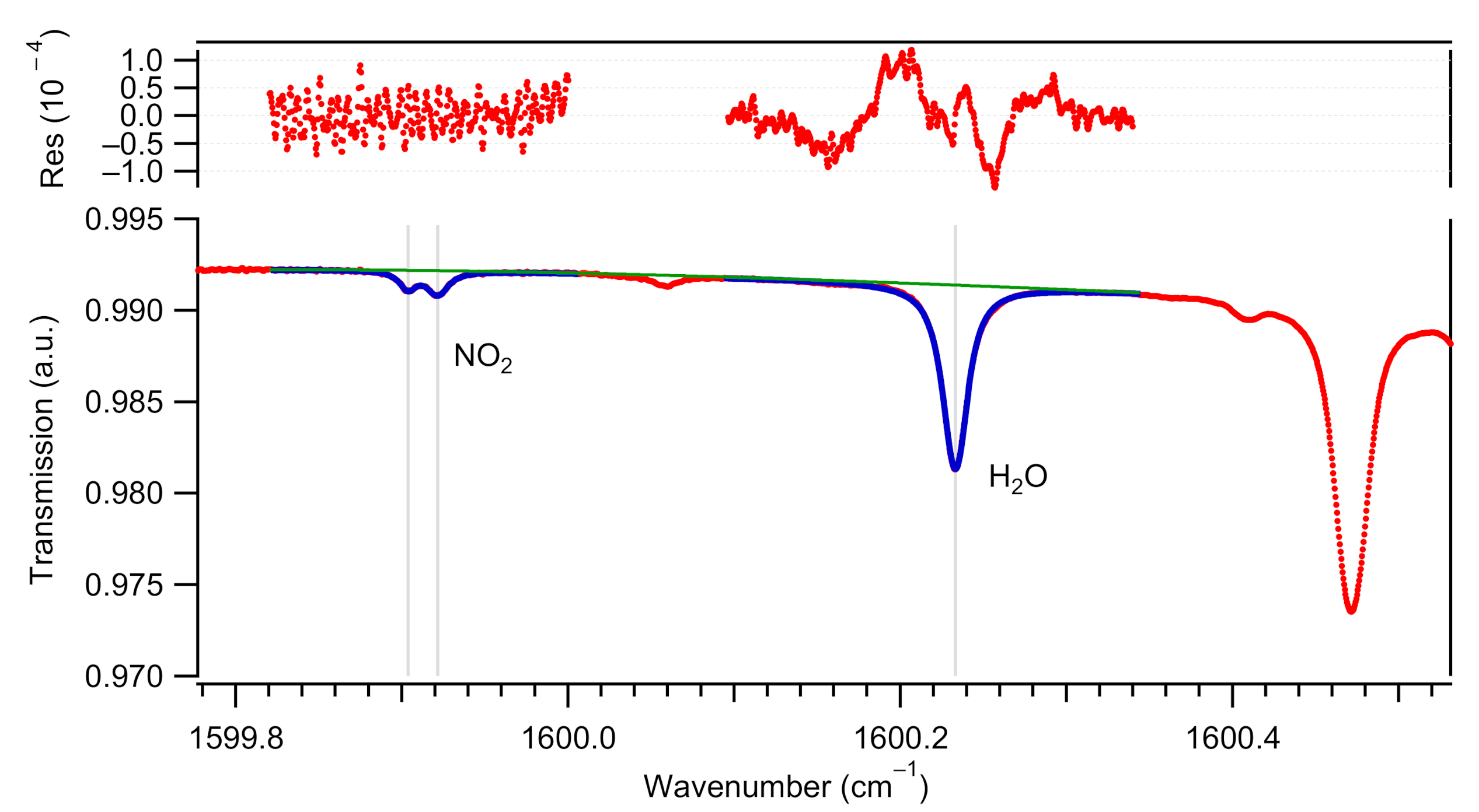
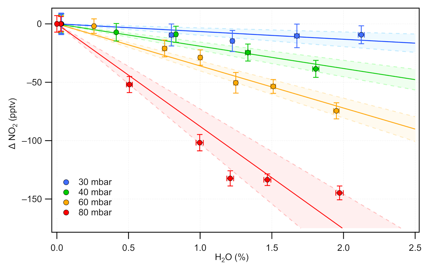
2.1.3. Spectral Interferences Induced by Water Vapor

Spectral simulations indicate that at sample pressures below 100 mbar, the ro-vibrational absorption lines of NO${}_2$ in the selected spectral region are sufficiently separated from lines of any other atmospheric species. In a previous study, however, Tuzson et al. [34] found that an ambient H${}_2$O amount fractions of 1% resulted in a NO${}_2$ equivalent signal of about −60 pptv compared to dry air measurements at the same gas pressure of 50 mbar. A similar water-induced bias has also been observed for our instrument. To precisely quantify this bias and mitigate its effect, different experiments at various water concentrations and at different sample pressures were conducted. The effect of humidity on the instrument’s NO${}_2$ retrieval was investigated by sampling alternatively dry and humidified synthetic air, both coming from the same source. The step-wise sample humidification was done by using a HovaCAL calibration gas generator (IAS GmbH, Iserlohn, Germany). A full cycle consists in measuring alternatively dry and humid samples, 3 min each. These experiments also showed that measuring dry air before and after several minutes of humid air sampling results in the same NO${}_2$ equivalent signal, which demonstrates the high inertness of the sampling line including the custom-made MPC.

Figure 6 shows the $\Delta$NO${}_2$, corresponding to the NO${}_2$ difference obtained between wet and dry conditions, in function of the H${}_2$O amount fraction (up to 2% absolute humidity) at different sample pressures ranging between 30 and 80 mbar. The water content was spectroscopically determined using the H${}_2$O line at 1600.25 cm${}^{-1}$ and calibrated against a dew-point hygrometer (Thygan VTP 6, Meteolabor AG, Switzerland). The data show that the NO${}_2$ equivalent signal clearly depends on the water amount fraction and the sample pressure. The observed NO${}_2$ bias at an absolute humidity of 1% is in a similar range as that found by Tuzson et al. [34]. This bias is attributed to a change in the spectral baseline due a very intense H${}_2$O absorption line located at 1601.2 cm${}^{-1}$. The tailing of the pressured broadened water absorption induces a steeper curvature of the baseline (compared to the dry situation) covered by the laser scan, causing an offset in the baseline intensity estimation at the NO${}_2$ line location. An increase in gas pressure causes a further broadening of this water line, thus enhancing this effect. Figure 6 shows that at 30 mbar and 1.5% humidity, the measured NO${}_2$ equivalent signal is approximately −10 pptv, which is close to the LOD of this instrument under typical operating conditions. The optimal operating parameters, however, depend on the measurement conditions: in remote, dry conditions (e.g., free troposphere), where NO${}_2$ and H${}_2$O amount fractions are both expected to be very low, working at an elevated gas pressure in the MPC ensures the highest possible precision, while near-ground measurements should be done at lower sample pressure to assure high selectivity. For the ambient measurements reported in Section 3.2, we used a simple linear function to determine the correction factor for the humidity effect.

2.2. Field Inter-Comparison Setup and Instrumentation

An inter-comparison between our custom-made QCLAS and three different commercial instruments took place in winter 2019/2020 at a suburban air quality monitoring station (47°24${}^{″}$09.2${}^{″}$ N, 8°36${}^{″}$51.9${}^{″}$ E) of the Swiss National Air Pollution Monitoring Network (NABEL) in Dübendorf, located 10 km southeast of the city of Zurich. The station consists of two rooms, main and annex, each having its own independent inlet of similar design and an air intake located 4 m above the ground and 1.5 m above the rooftop. The air intakes are horizontally separated by 5 m and therefore considered collocated. The gas flow through the inlet is 300 L/min and the corresponding residence time is about 1.2 s. Prior to the ambient air measurements, all NO${}_2$ instruments were calibrated with three different calibration methods (see Section 2.2.2). Ancillary measurements (temperature, humidity and O${}_3$) were provided by the NABEL.

2.2.1. Commercial NO${}_2$ Instruments

For the field campaign, we used the following commercial instruments: a CLD, a CAPS and another QCLAS. All instruments, apart from the CLD, and calibration units were located in the annex room of the monitoring station. The CLD device (T200 NO/NO${}_2$/NOx analyser, Teledyne Technologies Inc., Thousand Oaks, CA, USA) is the standard model used by NABEL, and it is permanently installed in the main room of the station. It uses a molybdenum converter to reduce ambient NO${}_2$ to NO. The instrument has a LOD of 200 pptv for NO${}_2$. The CAPS device (T500U NO${}_2$ Analyser, Teledyne Technologies Inc., Thousand Oaks, CA, USA) is based on NO${}_2$ light absorption at 450 nm in a resonant optical cavity and has a LOD of about 40 pptv. Both the CLD and the CAPS use a drier in their inlet to mitigate water interferences. The second QCLAS (NO${}_2$ Analyzer, MIRO Analytical AG, Dübendorf, Switzerland; hereafter, QCL-MIRO) is a newly available commercial instrument, which is based on the same technique as our custom-made QCLAS (hereafter, QCL-Empa). Furthermore, it also deploys the same laser-driving scheme, DAQ processes and spectral evaluation software [46], but it uses an NO${}_2$ absorption line around 1630 cm${}^{-1}$. The entire spectrometer is built into a 19”/4U rack and uses an AMAC-76 multipass cell (OPL = 76 m; Aerodyne Research Inc, Billerica, MA, USA). The LOD of this instrument is specified to 15 pptv. The instrument normal operation includes an automated re-zeroing cycle with 10 min period.

2.2.2. Calibration Methods

To ensure comparability between the NO${}_2$ instruments, they were all calibrated simultaneously prior to the ambient air measurements. During the calibration phase, each of the four instruments was sampling in parallel from the common calibration line. The CLD instrument was connected to this line via a 5 m ¼ inch PFA tubing. Three different calibration methods were applied: dilution of a 1 ppmv NO${}_2$ cylinder, gas phase titration of NO by ozone and permeation from a wafer type NO${}_2$ permeation tube.

The cylinder dilution calibration (CDC) was done using NO${}_2$ in N${}_2$ from a 10 L cylinder provided by the Dutch Metrology Institute (VSL, Delft, Netherlands), with a nominal concentration of 1.00 ± 0.04 ppmv (k = 2). The content of this cylinder was diluted by synthetic air to generate concentrations at the relevant range (from 0 to 100 ppbv). The 1 ppmv NO${}_2$ gas flow was controlled by a SilcoNert©2000 coated mass flow controller (MFC; range 0–500 mL/min, Vögtlin Instruments GmbH, Muttenz, Switzerland). The synthetic air flow was controlled by a second MFC (range 0–10 L/min, Vögtlin Instruments GmbH, Switzerland), both calibrated against a traceable Molbox system (Fluke Calibration, Everett, WA, USA). During the whole calibration phase, the dilution flow was kept constant at 5 L/min, and the 1 ppmv NO${}_2$ flow was varied step-wise between 0 and 500 mL/min. An overflow of about 1 L/min was located 2 m downstream of the mixing point to ensure constant pressure at the inlet of the NO${}_2$ instruments.

The gas phase titration (GPT) calibration was carried out using a 20 ppmv NO in N${}_2$ SI-traceable standard cylinder (50 L) from the National Physical Laboratory (NPL, Teddington, UK). The GPT reaction itself (NO + O${}_3$ = NO${}_2$ + O${}_2$) took place in a commercial GPT unit (MKAL-GPTM, BREITFUSS Messtechnik GmbH, Harpstedt, Germany), which includes an O${}_3$ lamp, a NO + O${}_3$ reactor and a dilution system. The total gas flow was kept constant at 5 L/min, and different NO${}_2$ concentrations were obtained by changing the light intensity of the O${}_3$ lamp. NO${}_2$ concentrations were retrieved from the NO concentrations measured with the CLD instrument, i.e., by assuming that the difference in NO concentration measured without and with the addition of O${}_3$ correspond to the NO${}_2$ concentration produced in the GPT instrument with a yield of 100%.

For the permeation calibration (ReGaS), a portable gas generator (ReGaS1) built by the Federal Institute of Metrology (METAS, Bern-Wabern, Switzerland) was used. This generator comprises a dilution system and a SilcoNert©2000 coated oven, with capacity for one permeation tube, similar to the ones described in Pascale et al. [47]. The delivered NO${}_2$ concentration depends on the permeation unit used, the oven temperature and the set flow. In this work, we used a NO${}_2$ permeation tube (VICI AG International, Schenkon, Switzerland) that had a permeation rate of 605 ng/min at 38 °C and 2.6 bar. This permeation tube was calibrated at the METAS using a magnetic suspension balance (TA instruments, New Castle, DE, USA) 9 months prior to the inter-comparison. The set concentration used in this work ranged from 20 to 65 ppbv with a total flow ranging from 4.5 to 5.3 L/min (with one or two dilution steps), from which at least 0.5 L/min was overflowing.

3. Results and Discussion

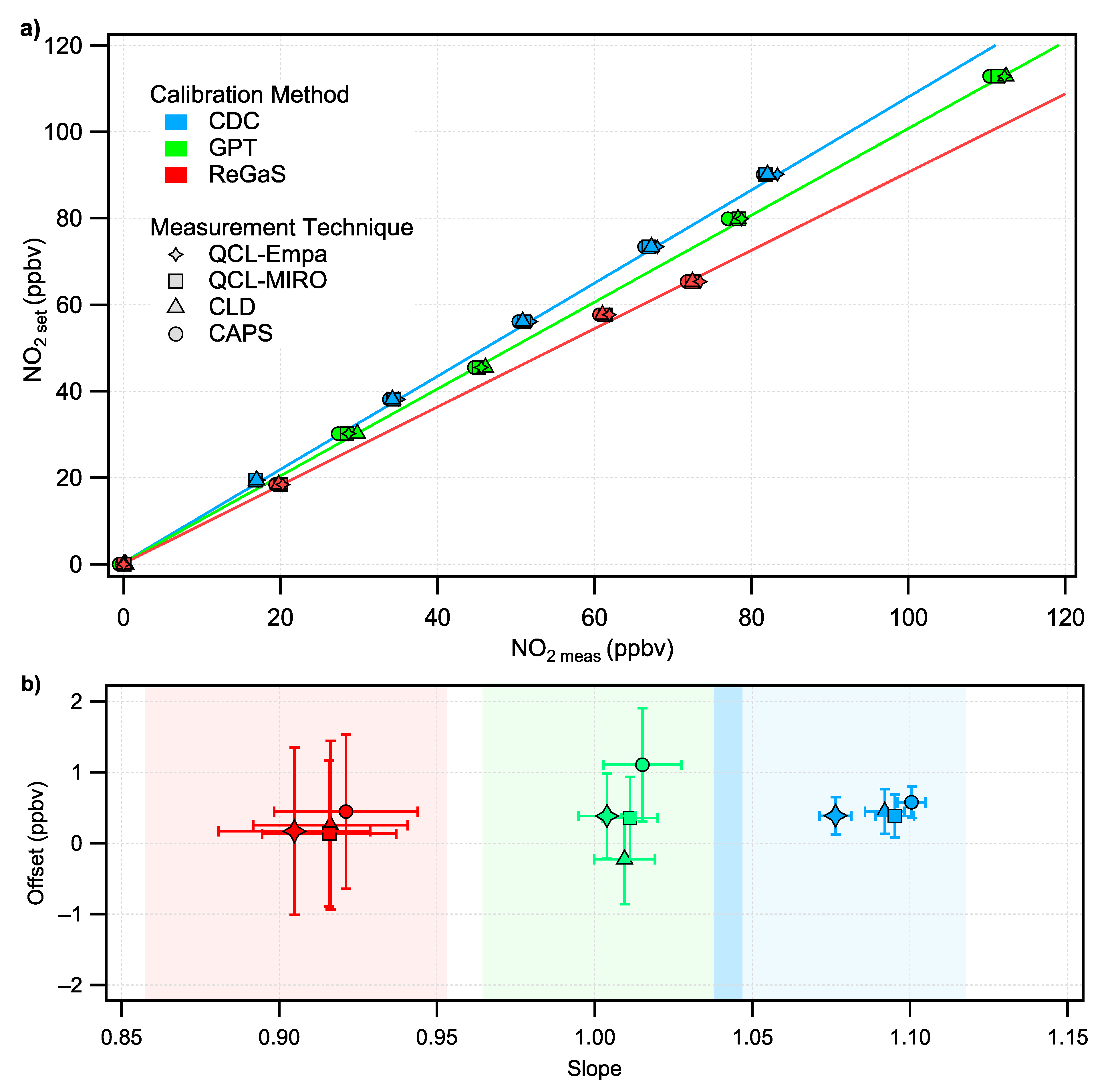
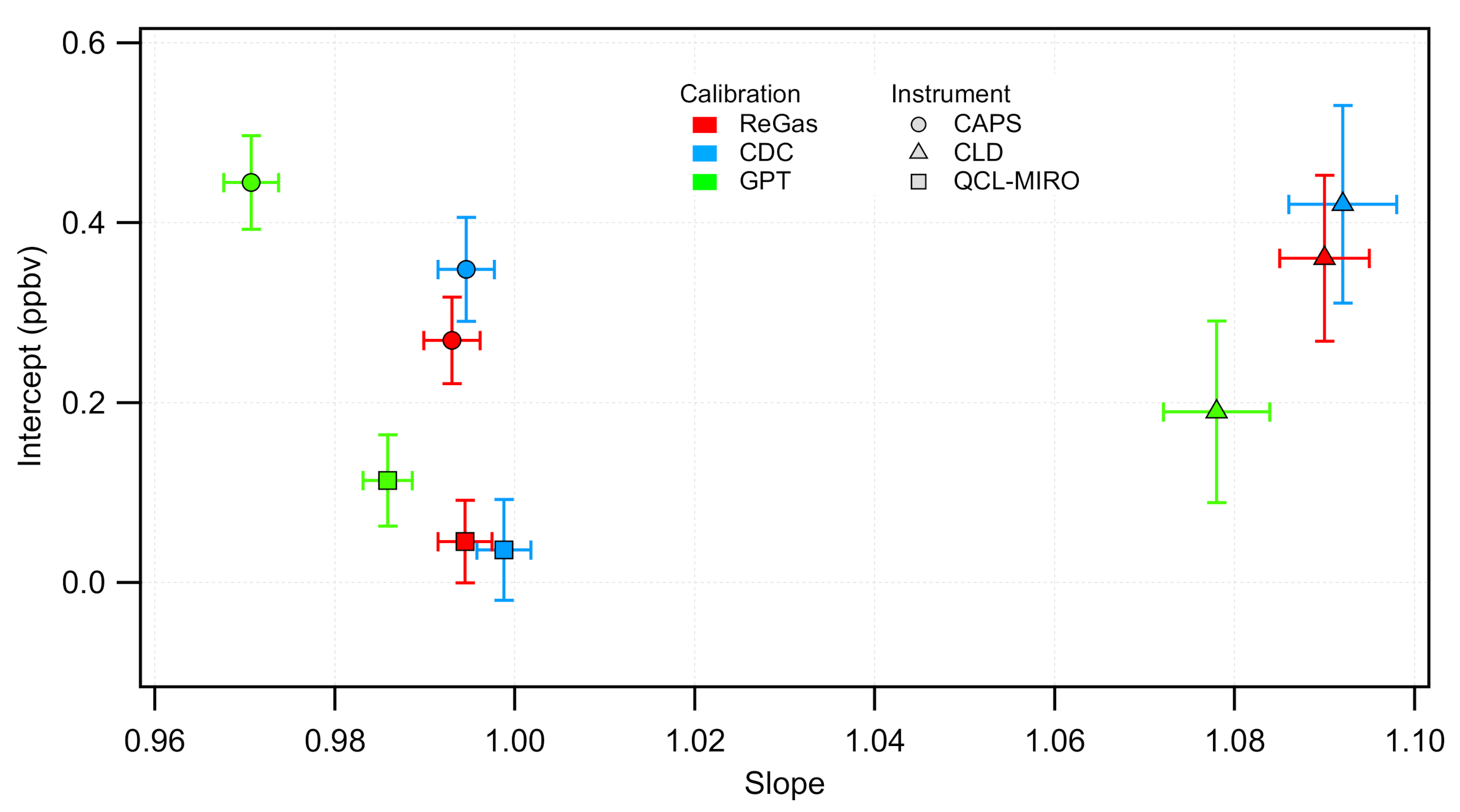
3.1. Calibrations of the NO${}_2$ Instruments

Figure 7a shows the results of all three different calibration methods performed prior to the ambient air measurement period (23 January–2 February 2020). The original calibration factors of the four instruments are based on different sources. The NO${}_2$ amount fraction reported by the QCL-Empa instrument was calculated solely based on the spectroscopic parameters using the HITRAN database and physical parameters (temperature, pressure and OPL). The CAPS and QCL-MIRO calibration parameters were preset by the instruments suppliers. The CLD calibration factors were based on calibration by a GPT unit similar to the one described in Section 2.2.2.

The calibration factors were obtained by a linear fit to these data using a least square method. The intercept of the linear regression is left to vary for all instruments, because they use different zeroing methods. The intercept and slope values determined from the regression analysis are shown on Figure 7b. The error bars represent the 2 $\sigma$ uncertainties of the fit. The width of the colored area represents the total uncertainty on the slope. It combines the uncertainty of the fit and that of the set span NO${}_2$ concentration (k = 2). The latter is estimated for each case separately: (i) for CDC, it takes into account the uncertainty of the MFCs flow and the NO${}_2$ cylinder concentration (≈4%); (ii) for GPT, the uncertainty is a combination of the NO measurement uncertainty of the CLD and the uncertainty on the NO cylinder concentration (≈2%); and (iii) the uncertainty on the ReGas method is a combination of the uncertainties of the permeation tube calibration and the MFC flows and considers environmental and temporal factors affecting the permeation rate [47]. The data in Figure 7 reveal a very good agreement (in terms of both the intercept and slope) between the NO${}_2$ instruments (within the uncertainties) despite their different ’factory’ calibration factors (based on either previous calibrations or purely spectroscopic data, such as for the QCL-Empa). On the other hand, significant discrepancies between the different calibration methods are observed. The average slopes (over the four instruments) for the CDC, GPT and ReGaS calibration are: 1.09, 1.01 and 0.92, respectively.

The higher slope values obtained with the CDC method compared to the established GPT method indicate an overestimation of the span NO${}_2$ concentration. This could be attributed to the long-term degradation of NO${}_2$ via gas phase reaction with water residuals or wall surfaces effect in the gas cylinder or to losses of NO${}_2$ on the internal surfaces of the pressure regulator of the cylinder. On the opposite side, calibration with the ReGaS instrument yields slopes values significantly lower than the GPT method. This implies an underestimation of the calculated set concentration (using the GPT as a reference). The latter is a function of the permeation rate (T and P dependent) and internal dilution factors. Potential errors in the calculation of the dilution factors alone are unlikely to explain the observed discrepancies with the established GPT method since they are based on mass flow readings with very low uncertainties [47]. The most probable source of error concerns the temporal gap between the permeation tube calibration and the inter-comparison campaign (9 months), the temperature readings in the permeation oven and the permeation tube purity indicated by the manufacturer. Another possible explanation for the lower slope values of the ReGaS calibration compared to the GPT and the CDC methods is that the latter two are subject to over-estimations of the set span concentration, for example due to losses of NO${}_2$, or, for the GPT, to an over-estimation of the conversion efficiency of NO.

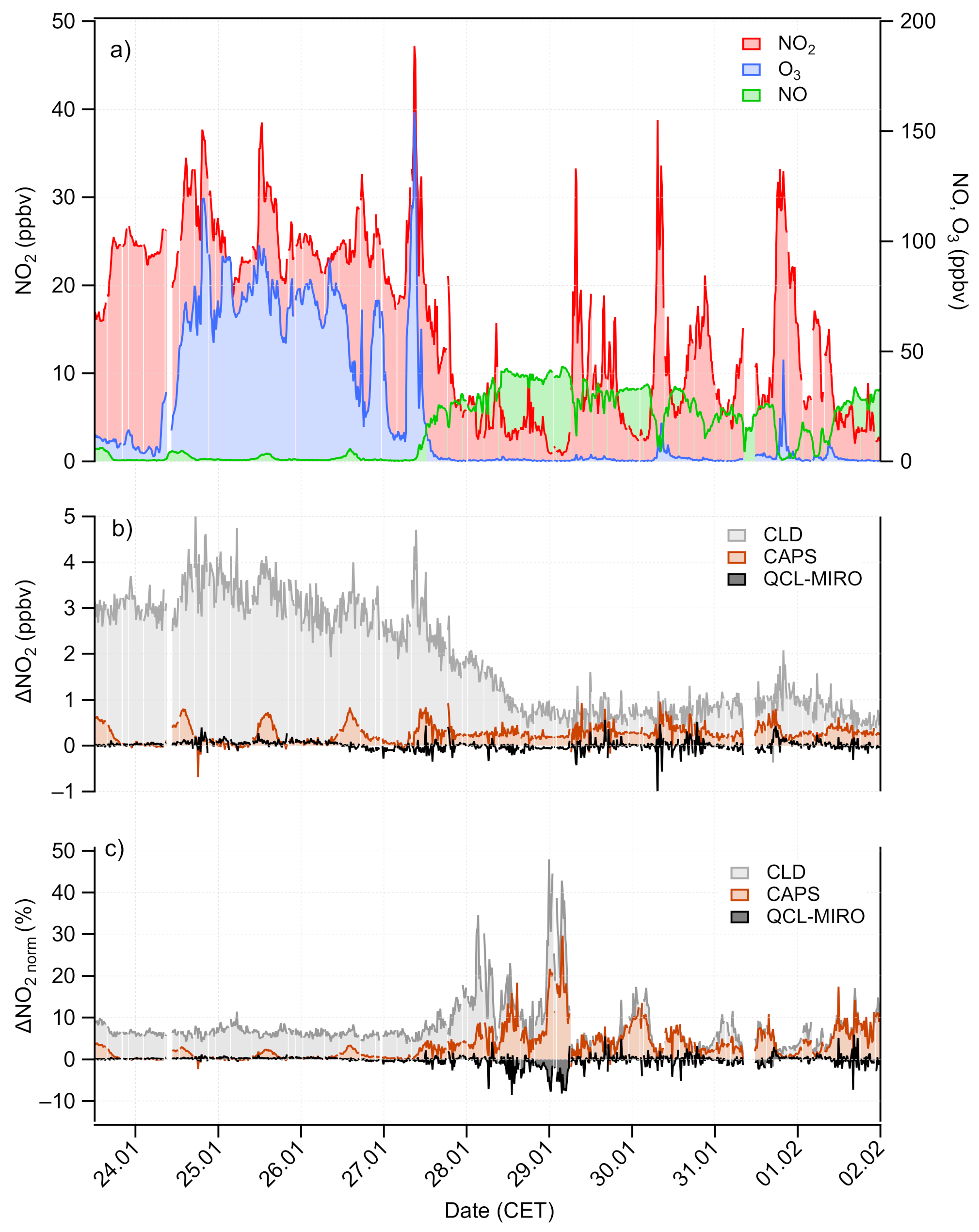
3.2. Ambient Air Measurements

Figure 8a shows the ambient NO${}_2$ amount fractions measurements for the 10 days of inter-comparison obtained by the QCL-Empa instrument, with the CDC calibration factors. We chose to present the data with these factors as they result in the highest ambient NO${}_2$ concentrations, which thus give the upper limit for the absolute differences between the instruments (Figure 8b). The amount fractions of NO (measured by CLD) and O${}_3$ are also shown. During the measurement period, the NO${}_2$ mixing ratios ranged from 0.5 to 50 ppbv, a high variability as expected from a site close to emission sources. In terms of O${}_3$ and NO${}_2$ concentration levels, the measurement period can be divided into two five-day sub-periods: the first period (24 January–27 January) is characterized by higher and more stable O${}_3$ and NO${}_2$ mixing ratios and much lower NO mixing ratios, while the second period (27 January–2 February) shows on average lower NO${}_2$, but with maximum values similar to the first period. The differences between the commercial NO${}_2$ instruments and the QCL-Empa measurements are shown in Figure 8b. The same differences normalized by NO${}_2$ (QCL-Empa) are presented in Figure 8c.

Besides the calibration factor, ambient air data were further corrected for formation of NO${}_2$ in the instruments individual inlet by the reaction between NO and O${}_3$. The amount of NO${}_2$ formed this way is estimated from the inlet residence time, the reaction rate constant between the reactants and their concentrations. The results of this calculation (in terms of NO${}_2$ amount fractions) were subtracted from the data of each instruments. The magnitude of this correction ranges from near 0 (mostly during night-time) up to 1 ppbv (for 6.5 s residence time in the CLD inlet line at 100 ppbv O${}_3$ and 5 ppbv NO). Finally, the QCL-Empa data were corrected for the H${}_2$O interference (see Section 2.1.3) using the correction factor determined at 60 mbar, the pressure used during the field measurements. This pressure was chosen as a comprise among precision, long-term stability and selectivity.

The agreement between the two QCL instruments is remarkable with an average normalized difference (Figure 8) of $-0.2\pm 1.4$%. This is not unexpected, since both instrument share largely the same technology. For the first period (having more stable and higher NO${}_2$ mixing ratios), the normalized difference is $0.1\pm 0.3$%. The CAPS is in reasonable agreement with the QCL-Empa with an average normalized difference of $3.4\pm 3.9$%. The main contribution to this difference lies in the offset of the CAPS measurements (compared to the QCL-Empa), as shown below. A closer look at the differences between the CAPS and the QCL-Empa measurements ($\Delta$NO${}_{2,CAPS}$, Figure 8b) reveals a diurnal cycle (with the highest contrast during the first period of the campaign, i.e., 23 January–27 January), with maxima corresponding to local noon-time, which correlate well with daily NO maxima. The first hypothesis to explain these observations is an erroneous estimation of the NO${}_2$ formed in the CAPS inlet. As the dominant part of the systematic error comes from the residence time calculation, we tested this hypothesis by calculating the extra (“missing”) time necessary to compensate for the $\Delta$NO${}_{2,CAPS}$. The corresponding values ranged from 0 to 5 s during the first period (23 January–27 January), corresponding to 0–100% increase of the initial estimation, to several several tens of seconds during the second period (27 January–2 February). Thus, the hypothesis can be rejected. Another possibility is the presence of an unaccounted light absorbent in ambient air. The $\Delta$NO${}_{2,CAPS}$ day/night time variations are stronger during the first part of the campaign that is impacted by higher ozone mixing ratios, which is a sign for stronger photo-chemistry. Previous studies have shown that dialdehydes absorb light in the wavelength range used by the CAPS instrument to detect NO${}_2$ [48,49]. The dominant ones in the troposphere, glyoxal and methyl-glyoxal, are produced by photo-chemical oxidation of hydrocarbons (mostly isoprene [50]), which is the same mechanism that drives the formation of ozone during daytime. These compounds are therefore good candidates to explain a positive bias in the CAPS instrument. The day/night cycle is in this case caused by the equilibrium between their sources and sinks, both dominated by photo-oxidation processes [51].

The strongest and most variable disagreement is found between the QCL-Empa and the CLD instrument, with a clear difference between the first and second periods of the campaign. The highest absolute and normalized differences are observed during the first measurement period, characterized by high O${}_3$ and low NO mixing ratios. These conditions are, as mentioned above, usually associated with photo-chemically aged air masses, while the second measurement period is likely dominated by freshly polluted air. This confirms the influence of more oxidized forms of nitrogen oxides on the NO${}_2$ measurement by CLD, which are usually found in higher concentrations in aged air masses.

The linear relationship between the NO${}_2$ instruments, after common calibration, on ambient air measurements is summarized in Figure 9. Each point corresponds to the intercept and slope of a linear fit between a given instrument and the QCL-Empa. All combinations of instruments and calibration techniques are presented, using the QCL-Empa as reference. The best agreement is obtained between the two QCL instruments using the calibration factors of the direct calibration methods (CDC and ReGaS), with offsets below 50 pptv and slopes between 0.995 and 1. The best correlation between the CAPS and the QCL-Empa is also obtained using the direct calibration methods, with slopes between 0.990 and 0.995. The fit, however, reveals a non-negligible offset of the CAPS data (between 250 and 350 pptv). The least agreement is obtained for the CLD instrument with slope values from 1.079 to 1.092 and offset values comprised between 200 and 425 pptv.

4. Conclusions

We designed a high-precision quantum cascade laser based mid-infrared spectrometer (QCLAS) for NO${}_2$ detection. The instrument reaches a precision (1 $\sigma$) of 0.8 pptv for NO${}_2$ after 150 s integration time. For this, we developed a fully custom-made astigmatic multipass absorption cell (MPC) with 110 m optical path length and employed a low-noise laser driver. The mirror design of the MPC involved optimization based on the investigation of simulated beam re-circulation patterns. The instrument’s response time (99%) is 45 s, which allows not only resolving rapid concentration changes, but also applying regular drift corrections by switching between sample- and zero-air measurements. This approach was demonstrated to maintain a limit of detection (LOD) for NO${}_2$ below 5 pptv, which complies with the highly challenging GAW data quality objectives. Furthermore, water-induced spectral interferences on NO${}_2$ detection were investigated under various humidity levels and pressure conditions. We show that operating the instrument at low sample pressure (30 mbar) allows minimizing the water induced bias near the LOD even for an absolute humidity of up to 2%. Furthermore, we show that the instrument can be operated in dual mode to simultaneously measure both NO${}_2$ and NO. The NO${}_x$ precision of 20 pptv after 150 s integration time can be be useful for ambient air quality monitoring and studies of the nitrogen cycle.

In addition, we also investigated different calibration methods (NO titration based, high-concentration cylinder dilution and permeation) during an inter-comparison campaign conducted at a suburban air quality monitoring station. We found significant differences between the calibration methods, which underlines the difficulty of handling NO${}_2$ and the importance of improved calibration methods. These discrepancies represent the main source of uncertainties of the measurements. The inter-comparison campaign involved the newly developed QCLAS as well as three other NO${}_2$ instruments: a chemiluminescence detector (CLD), a cavity attenuated phase shift spectrometer (CAPS) and a second QCLAS. While the two QCLAS instruments were in excellent agreement, the CLD showed a clear overestimation of the measured NO${}_2$ compared to the QCLAS. Significant and unexpected differences between the QCLAS and CAPS NO${}_2$ measurements were also observed. These were associated with photo-chemistry dominated conditions with a clear day/night cycle. Further measurements under various environmental conditions could help to validate the measurement quality of our instrument and to investigate biases on NO${}_2$ detection in the visible range.

Overall, our results demonstrate that QCLAS is a highly attractive alternative, in terms of both precision and selectivity, to existing instruments based on more commonly used techniques for NO${}_2$ detection.

References

1. Crutzen, P.J. Role of NO and NO2 in the Chemistry of the Troposphere and Stratosphere. Annu. Rev. Earth Planet. Sci. 1979, 7, 443–472. [Google Scholar] [CrossRef]
2. Monks, P.S.; Archibald, A.T.; Colette, A.; Cooper, O.; Coyle, M.; Derwent, R.; Fowler, D.; Granier, C.; Law, K.S.; Mills, G.E.; et al. Tropospheric ozone and its precursors from the urban to the global scale from air quality to short-lived climate forcer. Atmos. Chem. Phys. 2015, 15, 8889–8973. [Google Scholar] [CrossRef] [Green Version]
3. Lelieveld, J.; Gromov, S.; Pozzer, A.; Taraborrelli, D. Global tropospheric hydroxyl distribution, budget and reactivity. Atmos. Chem. Phys. 2016, 16, 12477–12493. [Google Scholar] [CrossRef] [Green Version]
4. Wayne, R.P.; Barnes, I.; Biggs, P.; Burrows, J.P.; Canosamas, C.E.; Hjorth, J.; Lebras, G.; Moortgat, G.K.; Perner, D.; Poulet, G.; et al. The Nitrate Radical - Physics, Chemistry, and the Atmosphere. Atmos. Environ. Part Gen. Top. 1991, 25, 1–203. [Google Scholar] [CrossRef]
5. Matsumaru, T.; Yoneyama, T.; Totsuka, T.; Shiratori, K. Absorption of Atmospheric NO2 by Plants and Soils. 1. Quantitative Estimation of Absorbed NO2 in Plants by N-15 Method. Soil Sci. Plant Nutr. 1979, 25, 255–265. [Google Scholar] [CrossRef] [Green Version]
6. Yoneyama, T.; Hashimoto, A.; Totsuka, T. Absorption of Atmospheric NO2 by Plants and Soils. 4. 2 Routes of Nitrogen Uptake by Plants from Atmospheric NO2 - Direct Incorporation into Aerial Plant-Parts and Uptake by Roots after Absorption into the Soil. Soil Sci. Plant Nutr. 1979, 26, 1–7. [Google Scholar] [CrossRef] [Green Version]
7. Schindler, C.; Ackermann-Liebrich, U.; Leuenberger, P.; Monn, C.; Rapp, R.; Bolognini, G.; Bongard, J.P.; Brandli, O.; Domenighetti, G.; Karrer, W.; et al. Associations between lung function and estimated average exposure to NO2 in eight areas of Switzerland. Epidemiology 1998, 9, 405–411. [Google Scholar] [CrossRef]
8. Barck, C.; Sandstrom, T.; Lundahl, J.; Hallden, G.; Svartengren, M.; Strand, V.; Rak, S.; Bylin, G. Ambient level of NO2 augments the inflammatory response to inhaled allergen in asthmatics. Respir. Med. 2002, 96, 907–917. [Google Scholar] [CrossRef] [Green Version]
9. Weinmayr, G.; Romeo, E.; De Sario, M.; Weiland, S.K.; Forastiere, F. Short-Term Effects of PM10 and NO2 on Respiratory Health among Children with Asthma or Asthma-like Symptoms: A Systematic Review and Meta-Analysis. Environ. Health Perspect. 2010, 118, 449–457. [Google Scholar] [CrossRef] [Green Version]
10. Reed, C.; Evans, M.J.; Di Carlo, P.; Lee, J.D.; Carpenter, L.J. Interferences in photolytic NO2 measurements: explanation for an apparent missing oxidant? Atmos. Chem. Phys. 2016, 16, 4707–4724. [Google Scholar] [CrossRef] [Green Version]
11. Saiz-Lopez, A.; Notario, A.; Albaladejo, J.; McFiggans, G. Seasonal variation of NOx loss processes coupled to the HNO3 formation in a daytime urban atmosphere: A model study. Water Air Soil Pollut. 2007, 182, 197–206. [Google Scholar] [CrossRef]
12. Li, J.Y.; Mao, J.Q.; Fiore, A.M.; Cohen, R.C.; Crounse, J.D.; Teng, A.P.; Wennberg, P.O.; Lee, B.H.; Lopez-Hilfiker, F.D.; Thornton, J.A.; et al. Decadal changes in summertime reactive oxidized nitrogen and surface ozone over the Southeast United States. Atmos. Chem. Phys. 2018, 18, 2341–2361. [Google Scholar] [CrossRef] [Green Version]
13. Stohl, A.; Trainer, M.; Ryerson, T.B.; Holloway, J.S.; Parrish, D.D. Export of NOy from the North American boundary layer during 1996 and 1997 North Atlantic Regional Experiments. J. Geophys. Res. Atmos. 2002, 107, 4131–4140. [Google Scholar] [CrossRef] [Green Version]
14. Parrish, D.D.; Ryerson, T.B.; Holloway, J.S.; Neuman, J.A.; Roberts, J.M.; Williams, J.; Stroud, C.A.; Frost, G.J.; Trainer, M.; Hubler, G.; et al. Fraction and composition of NOy transported in air masses lofted from the North American continental boundary layer. J. Geophys. Res. Atmos. 2004, 109, D09302–D09320. [Google Scholar] [CrossRef]
15. Gilge, S.; Plass-Duelmer, C.; Galbally, I.; Brough, N.; Bottenheim, J.; Flocke, F.; Gerwig, H.; Lee, J.; Milton, M.; Rohrer, F.; et al. WMO/GAW Expert Workshop on Global Long-term Measurements of Nitrogen Oxides and Recommendations for GAW Nitrogen Oxides Network; World Meteorological Organization (WMO): Geneva, Switzerland, 2011. [Google Scholar]
16. Fontijn, A.; Sabadell, A.J.; Ronco, R.J. Homogeneous Chemiluminescent Measurement of Nitric Oxide with Ozone-Implications for Continuous Selective Monitoring of Gaseous Air Pollutants. Anal. Chem. 1970, 42, 575. [Google Scholar] [CrossRef]
17. Miller, C.C. Chemiluminescence Analysis and Nitrogen-Dioxide Measurement. Lancet 1994, 343, 300–301. [Google Scholar] [CrossRef]
18. Winer, A.M.; Peters, J.W.; Smith, J.P.; Pitts, J.N. Response of Commercial Chemiluminescent NO-NO2 Analyzers to Other Nitrogen-Containing Compounds. Environ. Sci. Technol. 1974, 8, 1118–1121. [Google Scholar] [CrossRef]
19. Steinbacher, M.; Zellweger, C.; Schwarzenbach, B.; Bugmann, S.; Buchmann, B.; Ordonez, C.; Prevot, A.S.H.; Hueglin, C. Nitrogen oxide measurements at rural sites in Switzerland: Bias of conventional measurement techniques. J. Geophys. Res. Atmos. 2007, 112, D11307–D11320. [Google Scholar] [CrossRef] [Green Version]
20. Villena, G.; Bejan, I.; Kurtenbach, R.; Wiesen, P.; Kleffmann, J. Interferences of commercial NO2 instruments in the urban atmosphere and in a smog chamber. Atmos. Meas. Tech. 2012, 5, 149–159. [Google Scholar] [CrossRef] [Green Version]
21. Fuchs, H.; Ball, S.M.; Bohn, B.; Brauers, T.; Cohen, R.C.; Dorn, H.P.; Dube, W.P.; Fry, J.L.; Haseler, R.; Heitmann, U.; et al. Intercomparison of measurements of NO2 concentrations in the atmosphere simulation chamber SAPHIR during the NO3Comp campaign. Atmos. Meas. Tech. 2010, 3, 21–37. [Google Scholar] [CrossRef] [Green Version]
22. Rohrer, F.; Bruning, D. Surface NO and NO2 Mixing Ratios Measured between 30° N and 30° S in the Atlantic Region. J. Atmos. Chem. 1992, 15, 253–267. [Google Scholar] [CrossRef]
23. Mazurenka, M.I.; Fawcett, B.L.; Elks, J.M.F.; Shallcross, D.E.; Orr-Ewing, A.J. 410-nm diode laser cavity ring-down spectroscopy for trace detection of NO2. Chem. Phys. Lett. 2003, 367, 1–9. [Google Scholar] [CrossRef]
24. Kebabian, P.L.; Herndon, S.C.; Freedman, A. Detection of nitrogen dioxide by cavity attenuated phase shift spectroscopy. Anal. Chem. 2005, 77, 724–728. [Google Scholar] [CrossRef] [PubMed]
25. Osthoff, H.D.; Brown, S.S.; Ryerson, T.B.; Fortin, T.J.; Lerner, B.M.; Williams, E.J.; Pettersson, A.; Baynard, T.; Dube, W.P.; Ciciora, S.J.; et al. Measurement of atmospheric NO2 by pulsed cavity ring-down spectroscopy. J. Geophys.-Res.-Atmos. 2006, 111. [Google Scholar] [CrossRef] [Green Version]
26. Dhiman, C.; Khan, M.S.; Reddy, M.N. Phase-shift Cavity Ring Down Spectroscopy Set-up for NO2 Sensing: Design and Fabrication. Def. Sci. J. 2015, 65, 25–30. [Google Scholar] [CrossRef] [Green Version]
27. Kebabian, P.L.; Wood, E.C.; Herndon, S.C.; Freedman, A. A practical alternative to chemiluminescence-based detection of nitrogen dioxide: Cavity attenuated phase shift spectroscopy. Environ. Sci. Technol. 2008, 42, 6040–6045. [Google Scholar] [CrossRef]
28. Fuchs, H.; Dube, W.P.; Lerner, B.M.; Wagner, N.L.; Williams, E.J.; Brown, S.S. A Sensitive and Versatile Detector for Atmospheric NO2 and NOx Based on Blue Diode Laser Cavity Ring-Down Spectroscopy. Environ. Sci. Technol. 2009, 43, 7831–7836. [Google Scholar] [CrossRef]
29. Thieser, J.; Schuster, G.; Schuladen, J.; Phillips, G.J.; Reiffs, A.; Parchatka, U.; Pohler, D.; Lelieveld, J.; Crowley, J.N. A two-channel thermal dissociation cavity ring-down spectrometer for the detection of ambient NO2, RO2NO2 and RONO2. Atmos. Meas. Tech. 2016, 9, 553–576. [Google Scholar] [CrossRef] [Green Version]
30. Horii, C.V.; Zahniser, M.S.; Nelson, D.D.; McManus, J.B.; Wofsy, S.C. Nitric acid and nitrogen dioxide flux measurements: A new application of tunable diode laser absorption spectroscopy. Appl. Tunable Diode Other Infrared Sources Atmos. Stud. Ind. Process. Monit. 1999, 152–161. [Google Scholar] [CrossRef]
31. Sauer, C.G.; Pisano, J.T.; Fitz, D.R. Tunable diode laser absorption spectrometer measurements of ambient nitrogen dioxide, nitric acid, formaldehyde, and hydrogen peroxide in Parlier, California. Atmos. Environ. 2003, 37, 1583–1591. [Google Scholar] [CrossRef]
32. McManus, J.B.; Zahniser, M.S.; Nelson, D.D.; Shorter, J.H.; Herndon, S.; Wood, E.; Wehr, R. Application of quantum cascade lasers to high-precision atmospheric trace gas measurements. Opt. Eng. 2010, 49(11), 111124–111135. [Google Scholar] [CrossRef]
33. Lee, B.H.; Wood, E.C.; Zahniser, M.S.; McManus, J.B.; Nelson, D.D.; Herndon, S.C.; Santoni, G.W.; Wofsy, S.C.; Munger, J.W. Simultaneous measurements of atmospheric HONO and NO2 via absorption spectroscopy using tunable mid-infrared continuous-wave quantum cascade lasers. Appl. Phys. Lasers Opt. 2011, 102, 417–423. [Google Scholar] [CrossRef] [Green Version]
34. Tuzson, B.; Zeyer, K.; Steinbacher, M.; McManus, J.B.; Nelson, D.D.; Zahniser, M.S.; Emmenegger, L. Selective measurements of NO, NO2 and NOy in the free troposphere using quantum cascade laser spectroscopy. Atmos. Meas. Tech. 2013, 6, 927–936. [Google Scholar] [CrossRef] [Green Version]
35. Fehsenfeld, F.C.; Drummond, J.W.; Roychowdhury, U.K.; Galvin, P.J.; Williams, E.J.; Buhr, M.P.; Parrish, D.D.; Hubler, G.; Langford, A.O.; Calvert, J.G.; et al. Intercomparison of NO2 Measurement Techniques. J. Geophys. Res. Atmos. 1990, 95, 3579–3597. [Google Scholar] [CrossRef]
36. Zenker, T.; Fischer, H.; Nikitas, C.; Parchatka, U.; Harris, G.W.; Mihelcic, D.; Musgen, P.; Patz, H.W.; Schultz, M.; Volz-Thomas, A.; et al. Intercomparison of NO, NO2, NOy, O3, and ROx measurements during the oxidizing capacity of the tropospheric atmosphere (OCTA) campaign 1993 at Izana. J. Geophys. Res. Atmos. 1998, 103, 13615–13634. [Google Scholar] [CrossRef]
37. McManus, J.B.; Zahniser, M.S.; Nelson, D.D. Dual quantum cascade laser trace gas instrument with astigmatic Herriott cell at high pass number. Appl. Opt. 2011, 50, A74–A85. [Google Scholar] [CrossRef]
38. Fischer, M.; Tuzson, B.; Hugi, A.; Bronnimann, R.; Kunz, A.; Blaser, S.; Rochat, M.; Landry, O.; Muller, A.; Emmenegger, L. Intermittent operation of QC-lasers for mid-IR spectroscopy with low heat dissipation: tuning characteristics and driving electronics. Opt. Express 2014, 22, 7014–7027. [Google Scholar] [CrossRef] [Green Version]
39. Liu, C.; Tuzson, B.; Scheidegger, P.; Looser, H.; Bereiter, B.; Graf, M.; Hundt, M.; Aseev, O.; Maas, D.; Emmenegger, L. Laser driving and data processing concept for mobile trace gas sensing: Design and implementation. Rev. Sci. Instruments 2018, 89. [Google Scholar] [CrossRef] [Green Version]
40. Hundt, P.M.; Tuzson, B.; Aseev, O.; Liu, C.; Scheidegger, P.; Looser, H.; Kapsalidis, F.; Shahmohammadi, M.; Faist, J.; Emmenegger, L. Multi-species trace gas sensing with dual-wavelength QCLs. Appl. Phys. Lasers Opt. 2018, 124. [Google Scholar] [CrossRef]
41. McManus, J.B. Paraxial matrix description of astigmatic and cylindrical mirror resonators with twisted axes for laser spectroscopy. Appl. Opt. 2007, 46, 472–482. [Google Scholar] [CrossRef]
42. Gordon, I.E.; Rothman, L.S.; Hill, C.; Kochanov, R.V.; Tan, Y.; Bernath, P.F.; Birk, M.; Boudon, V.; Campargue, A.; Chance, K.V.; et al. The HITRAN2016 molecular spectroscopic database. J. Quant. Spectrosc. Radiat. Transf. 2017, 203, 3–69. [Google Scholar] [CrossRef]
43. McManus, J.B.; Nelson, D.D.; Herndon, S.C.; Shorter, J.H.; Zahniser, M.S.; Blaser, S.; Hvozdara, L.; Muller, A.; Giovannini, M.; Faist, J. Comparison of cw and pulsed operation with a TE-cooled quantum cascade infrared laser for detection of nitric oxide at 1900 cm-1. Appl. Phys. -Lasers Opt. 2006, 85, 235–241. [Google Scholar] [CrossRef]
44. Werle, P.; Mucke, R.; Slemr, F. The Limits of Signal Averaging in Atmospheric Trace-Gas Monitoring by Tunable Diode-Laser Absorption-Spectroscopy (TDLAS). Appl. Phys. -Photophys. Laser Chem. 1993, 57, 131–139. [Google Scholar] [CrossRef]
45. Li, Y.Q.; Demerjian, K.L.; Zahniser, M.S.; Nelson, D.D.; McManus, J.B.; Herndon, S.C. Measurement of formaldehyde, nitrogen dioxide, and sulfur dioxide at Whiteface Mountain using a dual tunable diode laser system. J. Geophys.-Res.-Atmos. 2004, 109, D16S08–D16S19. [Google Scholar] [CrossRef] [Green Version]
46. Hundt, P.M.; Muller, M.; Mangold, M.; Tuzson, B.; Scheidegger, P.; Looser, H.; Huglin, C.; Emmenegger, L. Mid-IR spectrometer for mobile, real-time urban NO2 measurements. Atmos. Meas. Tech. 2018, 11, 2669–2681. [Google Scholar] [CrossRef] [Green Version]
47. Pascale, C.; Guillevic, M.; Ackermann, A.; Leuenberger, D.; Niederhauser, B. Two generators to produce SI-traceable reference gas mixtures for reactive compounds at atmospheric levels. Meas. Sci. Technol. 2017, 28. [Google Scholar] [CrossRef] [Green Version]
48. Liu, J.W.; Li, X.; Yang, Y.M.; Wang, H.C.; Wu, Y.S.; Lu, X.W.; Chen, M.D.; Hu, J.L.; Fan, X.B.; Zeng, L.M.; et al. An IBBCEAS system for atmospheric measurements of glyoxal and methylglyoxal in the presence of high NO2 concentrations. Atmos. Meas. Tech. 2019, 12, 4439–4453. [Google Scholar] [CrossRef] [Green Version]
49. Min, K.E.; Washenfelder, R.A.; Dube, W.P.; Langford, A.O.; Edwards, P.M.; Zarzana, K.J.; Stutz, J.; Lu, K.; Rohrer, F.; Zhang, Y.; et al. A broadband cavity enhanced absorption spectrometer for aircraft measurements of glyoxal, methylglyoxal, nitrous acid, nitrogen dioxide, and water vapor. Atmos. Meas. Tech. 2016, 9, 423–440. [Google Scholar] [CrossRef] [Green Version]
50. Miller, C.C.; Jacob, D.J.; Marais, E.A.; Yu, K.R.; Travis, K.R.; Kim, P.S.; Fisher, J.A.; Zhu, L.; Wolfe, G.M.; Hanisco, T.F.; et al. Glyoxal yield from isoprene oxidation and relation to formaldehyde: chemical mechanism, constraints from SENEX aircraft observations, and interpretation of OMI satellite data. Atmos. Chem. Phys. 2017, 17, 8725–8738. [Google Scholar] [CrossRef] [Green Version]
51. Volkamer, R.; Molina, L.T.; Molina, M.J.; Shirley, T.; Brune, W.H. DOAS measurement of glyoxal as an indicator for fast VOC chemistry in urban air. Geophys. Res. Lett. 2005, 32, L08806–L08810. [Google Scholar] [CrossRef] [Green Version]
Figure 1. Top view of a 3D representation of the optical setup. Abbreviations: CLH, compact laser housing; BC, IR/IR beam combiner; TL, trace laser; FFM, flat flip-mirror; GE, germanium etalon; BSM, beam shaping in-coupling mirrors (f indicates the focal length of spherical mirrors); MPC, multipass cell (without closing lid); D, mid-infrared detector. The laser beam path from the CLHs to the first spot on the MPC’s back mirror and the path from the last spot to the detector are also indicated (colored line).
Applsci 11 01222 g001
Figure 2. Measured transmission spectrum (red dots, averaged over 10 4 spectral scans, corresponding to 1 s acquisition time) of an ambient air sample containing 10 ppbv of NO 2 and 0.1% (absolute) of H 2 O, along with the associated Voigt profile (blue line) and baseline fit (green line). The fit residual is shown on the top panel.
Applsci 11 01222 g002
Figure 3. Reflection spot patterns of the MPC. (a) (stars) Paraxial (transfer-matrix based) and (dots) non-paraxial (ray tracing) spot simulations on the front MPC mirror (with coupling hole) for the N366 and N274 patterns. (b) Simulated interference fringes spectrum for the N366 pattern based on the paraxial propagation simulation. The fringe intensities are given in arbitrary units. The number of passes corresponds to the fringe generating length. (c) Simulated and measured interference fringe spectra for the N274 pattern. Both simulated spectra are normalized to the simulated fringe intensity at 22 passes. Similarly, the measured spectrum is normalized to the measured fringe intensity at 22 passes.
Applsci 11 01222 g003
Figure 4. Allan–Werle deviation plot (1 σ ) of 12 h measurements of NO 2 equivalent amount fraction obtained by sampling NO 2 -free synthetic air at different sample pressures (30 and 80 mbar) and two distinct operation modes (NO x and NO 2 mode).
Applsci 11 01222 g004
Figure 5. Zero-drift corrected and 1 min averaged time-series of 12 h long measurements of synthetic air using two different sample pressures (30 and 80 mbar) and duty cycles of 50% and 90%, respectively. The associated histograms with a Gaussian fit indicate the spread of the data for each cases.
Applsci 11 01222 g005
Figure 6. Influence of water vapor on the retrieved NO 2 amount fraction. The negative bias ( Δ NO 2 , corresponding to the difference between wet and dry conditions) is plotted as a function of the absolute humidity of the sample at different pressures. The confidence intervals (± 95%) of the linear regressions are indicated by shaded areas. The error bars indicate the 1 σ standard deviation of the measured Δ NO 2 and the uncertainties of the water measurements (k = 1).
Applsci 11 01222 g006
Figure 7. Calibration results: (a) Set versus measured NO 2 amount fractions for the four instruments and the three different calibration methods deployed. The colored lines show the least squares linear regression for the QCL-Empa instrument. (b) Summary of the intercepts and slopes of the linear fit of the data in (a). The error bars represent the 2 σ uncertainties of the fit. The width of the colored area represent the combined uncertainty of the fit and of the set span NO 2 concentration for the QCL-Empa calibration (k = 2).
Applsci 11 01222 g007
Figure 8. Time-series measured during the field campaign: (a) ambient NO 2 (measured by the QCL-Empa with the CDC calibration factor), NO (measured by the CLD) and O 3 ; (b) absolute differences between NO 2 measured by the CLD, CAPS and QCL-MIRO and the QCL-Empa; and (c) absolute differences normalized by the NO 2 (QCL-Empa) values (the CLD data being further divided by two, for better visibility).
Applsci 11 01222 g008
Figure 9. Intercepts and slopes of the linear regression of ambient air measurement data for the CLD, CAPS and QCL-MIRO vs. the QCL-Empa using three different calibration methods. The error bars represent the fit uncertainties (1 σ ).
Applsci 11 01222 g009