
Review on System Identification and Mathematical Modeling of Flapping Wing Micro-Aerial Vehicles

1
Center for Advanced Studies in Telecommunications, COMSATS Institute of Information Technology, Islamabad 45550, Pakistan
2
School of Mechanical Engineering, The University of Adelaide, Adelaide, SA 5005, Australia
*
Author to whom correspondence should be addressed.
Appl. Sci. 2021, 11(4), 1546; https://0-doi-org.brum.beds.ac.uk/10.3390/app11041546
Submission received: 31 October 2020
/
Revised: 21 January 2021
/
Accepted: 22 January 2021
/
Published: 8 February 2021
(This article belongs to the Special Issue Bioinspired Flight)
Abstract
:Featured Application
The paper provides a comprehensive review on various system identification and modeling techniques for flapping wing micro-aerial vehicles (FWMAVs) that will be useful for researchers in order to obtain mathematical modeling of FWMAVs.
Abstract
This paper presents a thorough review on the system identification techniques applied to flapping wing micro air vehicles (FWMAVs). The main advantage of this work is to provide a solid background and domain knowledge of system identification for further investigations in the field of FWMAVs. In the system identification context, the flapping wing systems are first categorized into tailed and tailless MAVs. The most recent developments related to such systems are reported. The system identification techniques used for FWMAVs can be classified into time-response based identification, frequency-response based identification, and the computational fluid-dynamics based computation. In the system identification scenario, least mean square estimation is used for a beetle mimicking system recognition. In the end, this review work is concluded and some recommendations for the researchers working in this area are presented.
1. Introduction
The fascination toward the flight of natural fliers has inspired the development of flapping-wing micro air vehicles (FWMAVs). Natural fliers, particularly of insect types, offer interesting flight mechanisms and aerodynamics that have not been completely understood until today. The currently estimated more than ten million insect’s species [1] include flies, which change their flight conditions based on some specific arrangements of their wing strokes [2,3], offer different adjustments of the wings that make the insects capable of flying with extreme maneuverability and impressive stability [1,4,5] compared to the conventional fixed wing aircrafts [6,7]. Some characteristics like their dexterity, broad flight envelope, robust behaviors in different situations at very low Reynolds numbers, hovering ability, the ability of quick transition to forward flight, abrupt maneuvers, make FWMAVs potentially beneficial in this era. Insect fliers generally use elastic elements in their flight muscles as energy storage and thus, minimize their inertial power, thus enhancing their power loading [8]. This results in a more efficient flight, which is another advantage of flapping-wing flight over rotary wings [9]. Exhaustive applications of such MAVs can be found, for example, as a reconnaissance platform for search and rescue as well as military operations. Fitted with a camera, FWMAVs can be deployed in risky and hazardous conditions such as after natural catastrophes to quickly determine and monitor the situation, for finding routes, identify potential dangers, and patrol border lines for security purposes as well as for civil applications such as the remote inspection of pipes and power lines, inspection of crop fields, and the conditions for fertilization and harvesting [10,11,12,13].
Based on the current trends, it is envisioned that FWMAVs will dwell in the gaps between the rotary and fixed wing aircraft because of their aforementioned appealing characteristics. In this context, micro- and nano-flapping wing fliers [10,11,12,13,14,15,16,17,18,19,20] are also believed to provide a wide number of advantages with considerably low cost and flight efficiency. As shown in [21], insect flights show higher power loading than multi-rotor drones. However, for FWMAVs, the small size of the sensors and mass restricts the onboard processing. Furthermore, depending on the overall size of the MAVs, the limited choice of small size onboard power supplies often means that the flight duration is a relatively short period in comparison with other types of aircraft. Thus, at the present stage of development, such efficiency has yet to be achieved. Therefore, energy efficient flight, attitude determination, and flight control of FWMAVs are still the main focus of researchers, scientists, and engineers [13,16].
FWMAVs are primarily recognized and developed into two classes (i.e., tailless and tailed). The tailless designs usually mimic the insects, which, consequently, provide high dynamic maneuvers. These configurations, in general, require active stabilization because they can be found passively unstable in forward flight and hovering [22]. In such developments, the nano-hummingbird [7] and robotic bee, known as RoboBee [10], have shown actual flight stability. On the other hand, the tailed design is found to be similar to configurations in birds, which are known for being passively stable, and therefore do not require active stabilization [15,23]. This kind of configuration provides the ease to develop and implement higher-level problems like altitude stabilization [24,25] and obstacle avoidance [25,26,27]. Figure 1 displays some of the well-known flapping-wing micro air vehicles that have been developed to date.
It is witnessed in Figure 1 that these FWMAVs differ in design as well as in its flying mechanism. The FWMAVs (Figure 1a,b,f,h) follow very similar flight mechanics as birds. This class utilizes the surface control mechanism for different maneuvers like pitching, rolling, yawing, and hovering. The surface motion control resembles the fixed wing aircraft strategies [7], whereas the FWMAVs in (Figure 1c,d,e,g) mimic the insects flying mechanism to experience different flight maneuvers [11,14,15,16,19,20,28,29]. The autonomous flight of the first category is relatively easier compared to that of the second class of FWMAVs. A clear understanding of insect flight depends on subtle details that might be easily overlooked in otherwise thorough theoretical or experimental analyses. Recently, researchers have benefited greatly from the use of high-speed cameras for capturing wing kinematics, new strategies such as digital particle image velocimetry (DPIV) to quantify flows, and powerful computers for further computational analysis. With the help of these methodologies, one can develop more accurate and rigorous models of these insects while having a fewer number of assumptions in developing wing kinematics, aerodynamics, and flight dynamics.
Despite the challenges faced in conducting experiments to quantify the wing motions of several flying insects due to their small size and high wing beat frequencies, insect fliers’ flapping kinematics, particularly that of free hovering flight and free forward flight, have been well-researched for more than 50 years. Early attempts to capture free-flight wing kinematics such as Ellington’s comprehensive and influential survey [30] relied primarily on a single-image high-speed cine. Although quite informative, especially because digital imaging technology continues to offer exceptional spatial resolution, single-view techniques cannot provide an accurate time course of the angle of attack of the wings. More recent methods have employed high-speed videography [31], which offers greater light sensitivity and ease of use, albeit at the cost of image resolution. A further consideration is that insects rely extensively on visual feedback, and hence, care must be taken to ensure that lighting conditions do not significantly impair an insect’s behavior. Even more challenging than capturing wing motions in 3-D is measuring the time course of aerodynamic forces during the stroke. At best, flight forces have been measured on the body of the insect rather than its wings, making it very difficult to separate the inertial forces from the aerodynamic forces generated by each wing [32,33,34,35,36]. In addition, unlike in free flight conditions, tethering can alter the wing motion, and thus, modify the generated forces. Researchers have overcome these limitations using two strategies. The first method involves constructing dynamically scaled models on which it is easier to directly measure aerodynamic forces and visualize flows [37,38,39,40,41,42,43]. A second approach is to construct computational fluid dynamic simulations of flapping wings [44,45,46,47,48]. The power of both approaches, however, depends critically on accurate knowledge of wing kinematics.
In general, to understand the mechanics of flapping wing flight, three basic aspects need to be well understood: flapping kinematics, aerodynamics, and flight dynamics (a detailed summary can be found in [49,50,51]). Several attempts have been made to model FWMAVs based on the knowledge of those three aspects of natural fliers such as those in [52], which focused on the first principle approach of modeling that includes flight stability and control. However, since FWMAVs depend on the flapping mechanism, the actuation system for generating the aerodynamic forces and moments as well as the sensors and control dynamics, mathematical models of FWMAVs solely based on the first principles may not accurately describe the actual dynamics of the MAVs. The review provided in this paper is intended to give insights into system identification approaches as an alternative way in obtaining mathematical models of various FWMAVs based on experimental data. Such approaches differ from the conventional modeling approaches through physics (i.e., modeling through the first principles). With system identification approaches, the richness of experimental or flight data can be exploited to obtain the flight dynamics and aerodynamics characteristics of FWMAVs. The models obtained through such approaches can be used to validate mathematical models (including those obtained through the first principles) and predict the effect of any design changes.
System identification uses mathematical modeling techniques, which are based on observed input–output data. This process was first coined by Lofti Zadeh in the late 1950s [53]. It has been used successfully to identify models of various complex systems such as the cardiovascular system [54], aircraft [55,56], and underwater vehicles [57]. This type of modeling approach is beneficial in developing realistic mathematical models of complex systems based on experimental data for prediction, simulation, system design, and/or control [58]. System identification is usually conducted via (1) the Black box approach in which system identification is carried out by fitting the system’s input–output response with some flight data, or (2) the Grey box approach (see [59] for more details), which is carried out by first developing the structure of models mathematically, then the required parameters in the models are identified. In both approaches, the overall models are validated against the experimental data. The typical steps involved in system identification are shown in Figure 2.
In this paper, the most prominent strategies relevant to system identification of the flight dynamics and aerodynamics of FWMAVs as well as natural fliers were overviewed. This paper is organized as follows. A general description of FWMAVs is presented and some major works done so far are highlighted in the Introduction. In Section 2, the background of the flight of FWMAVs is presented comprehensively and recent developments in this area are highlighted. Section 3 contains a brief discussion on system identification approaches, which then leads to the main review that presents different strategies in system ID adapted for modeling the FWMAVs’ dynamics. The article is presents our concluding remarks and some recommendations in Section 5, where the authors present their own proposed strategy for an online system’s stability derivative estimation that is potentially advantageous in obtaining the flight dynamics of any existing FWMAVs as future works.
2. Micro-Aerial Vehicle Flight
Current developments in flapping wing MAVs, which are inspired by natural fliers, can be categorized into two classes: bird (or vertebrate) flight and insect flight [60]. Although in general, both types of natural fliers observe three types of flight, which are named as gliding flight (mostly found in vertebrate flight), forward flight, and hovering [12,61,62,63,64,65,66], there are differences in their aerodynamics (see Figure 3). In bird flight, the wings generally have two degrees of freedom (i.e., the flapping and symmetric twisting of the wings downward and upward, i.e., pronation and supination occur respectively) to change the angle of attack and the lift. However, in the second class, the wings follow three degrees of motion (i.e., the main flapping motion is defined along the body axis with a certain stroke plane, while flapping the wing exhibits pitching motion along its root and experiences deviation from the stroke plane). In other words, while flapping, the wings follow an eight like pattern, which is, by definition, a two-degree motion [52]. Consequently, a three degree of motion occurs. The wing strokes are divided into upstroke and downstroke that are further categorized into normal rotation, advanced rotation, and delayed rotation. The wing rotation is termed as normal if the rotation occurs at the end of each half stroke, the rotation is advanced if it occurs before the end of the half stroke and after the mid stroke, and delayed rotation occurs after the half stroke and before the mid stroke. Furthermore, the normal rotation is, once again, recognized as water treading and normal hovering (for more details see [60,67,68]). Detailed comparison between the vertebrate and insect flights can be found in [69,70].
In the context of understanding the aerodynamics and wing kinematics, the lift and power requirement analysis related to hovering natural fliers (e.g., hummingbird and Drosophila family) was conducted in seminal works [73,74], which was further refined in the work of Ellington [30,75,76,77,78,79]. These pioneering works were further developed for other species, which include the design of some morphological parameters and wing kinematics (e.g., hawkmoths [80,81], dragonflies [82,83], bumblebee [84,85], robotic bee [10,20], and the beetle [11]. The flight characteristics are modeled in terms of aerodynamics and wing kinematic models. In the existing literature, two main strategies have been extensively studied for the development of the aerodynamic models (i.e., blade element methodology (BEM) and Navier–Stokes equation) through the computational fluid dynamics (CFD) strategy. The blade element strategy based aerodynamic models was developed in [61,68], where they incorporated the unsteady and added mass effects. The progress in the aerodynamics modeling in the last decades is comprehensively presented in [52,86,87,88,89,90,91,92].
In recent developments, [93,94] tried to abridge the theoretical and experimental strategies and to develop a standard linear aerodynamic model for DelFly II. The developments were mainly based on the standard aircraft system identification techniques and their extension to FWMAVs, which can be further used for simulation and autonomous full flight envelope. In [95,96], a two-dimensional flapping wing was considered, and the aerodynamic performance in asymmetric stroke in hovering and forward flight was numerically studied. In addition, the analysis of the effects of the asymmetry of the stroke on the aerodynamic forces and flow structures was carried out. The authors in [97] carried out a BEM for the development of the fluid–structure interaction model by synthesizing it with a structural model. The benefits of this strategy were that it not only improved the reliability of the BEM, but it also enabled various aerodynamic studies (e.g., [98,99,100,101,102]). Note that the BEM method is widely utilized due to its simplicity and robustness, however, its accuracy has been questioned. In contrast, computational simulations based on the solution of Navier–Stokes equations [103,104,105] have been utilized because they provide, with relatively high accuracy and precision, the detailed flow structures, time-dependent aerodynamic forces, and power requirements. However, this strategy needs high-fidelity modeling and a long experiment processing time, which in turn diminishes its usage in practice.
A CFD-informed quasi-steady model based on a hybrid of high- and low-fidelity models to reduce the aforementioned complexity was presented in [106]. The systematic development regarding the beetle’s and DelFly II’s aerodynamics can be found in [107,108,109], respectively. In order to update the research carried out in the area of FWMAVs, a comprehensive bibliometric review can be found in [110]. The flight stability of different species of natural fliers, particularly the longitudinal stability, was studied successfully by a number of researchers, for example, the stability of desert locust Schistocerca Gregaria was thoroughly presented in [86], the nano-humming bird was focused on in [12], insects mimicking the FWMAV’s initial stability was addressed in [111], and bumblebee stability was presented in [112]. In general, the eigenvalue-based analysis resulted in three modes common to all fliers, namely, the unstable oscillatory mode, stable fast subsidence mode, and stable slow subsidence mode. Almost all mathematical models developed in the aforementioned studies fall in the category of modeling by the first principles. System identification approaches have hardly been used. Therefore, the forthcoming section will present, in detail, the techniques devised for system identification approaches, particularly, in obtaining system stability derivatives and control-oriented dynamic models of FWMAVs and natural flapping fliers.
3. System Identification and Mathematical Modeling of Flapping Wing Micro Air Vehicles (FWMAVs)
The ultimate objective, in the development of FWMAVs, is securing an autonomous flight in order to utilize them for the different tasks mentioned earlier. Therefore, a first step toward the establishment of an autonomous flight is the modeling of the flapping kinematics, aerodynamics, and flight dynamics of FWMAVs. This task is particularly challenging due to inherent instability, nonlinear, time-varying, and periodic nature of the vehicles’ dynamics, especially during dynamic aerial maneuvers such as sharp and abrupt turns, obstacle avoidance, and mid-air prey capturing. The aerodynamics and flight dynamics of such maneuvers, even for natural fliers, have not been fully uncovered yet. Additionally, on-board sensors, flapping mechanism, and actuation systems may add complexities to the overall dynamics of the MAVs. Furthermore, for insect-mimicking FWMAVs, due to their small size, the selection of hardware for their avionics and flight control systems are limited. However, in this review, we focused on system identification approaches in order to model the FWMAVs without actually going through the details on hardware selection.
In general, two complementary strategies are applied to model FWMAVs. These strategies are named as bottom-up and top-down [94]. The bottom-up approach mainly focuses on the fundamental approaches to explain and model the behavior and interaction of air motion with the flapping wings. This is essentially modeling with the first principles based on the well-studied aerodynamics and wing kinematics of natural flapping fliers (see [50] for a detailed summary). The practical system development of bio-inspired FWMAVs remains the later part in such developments. On the other hand, in the top-down approach, the construction and developments of the real MAVs take place prior to the theoretical developments. In order to obtain the mathematical model(s) of the FWMAVs, the first step is the system identification, which means a strategy for acquiring a known mathematical model (for instance, aerodynamic modeling, system stability derivatives, and system’s control derivatives) of the system while utilizing the available measured data of the system’s input and output signals produced by the MAVs. These available signals may be measured either in time domain or in frequency domain. The main advantages of performing system identification in modeling are that the process uses real-time data and can take into account design changes. The latter is particularly useful for control system design. Through the process, the value of specific design parameters and their effects on the dynamics of MAVs can be determined, and the structure of the mathematical models obtained is not unique, which gives the freedom to the engineers/researchers to select the models that suit the objectives of the modeling. For examples, these models may be suitable for (hardware-in-the-loop) simulations, analysis, and/or control.
With regard to this stage, the FWMAVs and their flight have been enlightened in a general way, and now the objective is to present the system identification in detail. It is generally conducted either for equivalent linear systems or core nonlinear systems. This may further be classified into time-domain and frequency-domain based identification for tailed and tailless FWMAVs. It is obvious that the dynamic modeling of FWMAVs always considers the mechanism kinematics of linkages, which connect the motors and actuators to FWs [113], aerodynamic forces [114], and nonlinear phenomena like saturation and hysteresis [115]. Consequently, it results in different equations and realizations of the dynamics.
The linear modeling and identification of fixed wing aircraft were extensively studied in [55,114]. The identification strategies for modeling FWMAVs or natural fliers vary from system to system because of their varying kinematics and flight dynamics. The review paper by [52] highlighted that the inertia effects of the wings on the main body were invoked in very few models of the flapping wing systems. The majority of the flapping angles of FWs remains greater than 20 degrees (see, for instance, [116]). Therefore, the small angle assumption (i.e., ) is no longer valid, and consequently, the linearized dynamic model becomes inaccurate. The dynamic models of the FWs are generally highly nonlinear and time varying due to the aerodynamic forces on the wings that are typically predicted via the lift and drag coefficients of the quasi-steady aerodynamic model. These coefficients depend on the angle of attack, which may vary significantly during a single stroke. Various nonlinear modeling approaches have focused on the addition of a spring in the redesign and optimization of the elastic elements like actuators, wings, and linkages to further improve the capability of the system to be driven at resonances [16,17,18,19]. Another strategy [20] considered wing, actuator, and transmission components, and developed an integrated nonlinear model, which considers all the changes made in the wing shape and linkage system. The change in the wing shape significantly affects the inertial properties and the aerodynamic damping forces, whereas the variation in the linkage mechanism affects the control input channels. Some useful linear models have also been developed that account for the nonlinear geometric and aerodynamic components [117,118]. The developed nonlinear model sufficiently predicts the behavior of the FWMAVs with a considerable operating range. However, the accuracy in the model reduces when operated at high frequencies.
The FWMAVs, as mentioned earlier, mimic either insect or bird flight. They are stabilized via active and passive stabilization strategies in different flight envelopes [10,12,30,31,32] through manually tuned controllers such as proportional-derivative (PD) and/or proportional-integral-derivative (PID) controllers. However, they are observed to be sensitive to external disturbances. Thus, it becomes quite challenging to keep them stable in broad flight envelopes. One reason for such difficulties is the absence of a sufficiently accurate nonlinear model that can describe the unsteady aerodynamics of the FWMAVs’ flapping motions [119,120] and the added inertia effect contribution to the MAVs dynamics [121]. In this context, a linear time invariant (LTI) model was developed in [121,122,123,124] via the use of standard aircraft equations. Another approach, known as the multi-body approach, was introduced. However, such an approach for a time varying nonlinear model [121,125] is not suitable for onboard processing. All the aforementioned approaches have significant shortcomings such as a lack of practical validation, limited only to computational environment and the repeatability of the data. Therefore, it is demanding to overcome such modeling difficulties in order to fully explore the capabilities of these fliers.
In the subsequent subsections, we will focus on system identification strategies that have been applied for identifying parameters and mathematical models of FWMAVs. In presenting the review, we classify natural fliers and FWMAVs into two categories, the tailed and tailless fliers/FWMAVs. Various system identification techniques used in identifying the model parameters of fliers/FWMAVs in these two categories will be discussed.
3.1. Tailed Flapping Wing Micro-Air Vehicles
In this section, we intend to present the details of system identification techniques for tailed micro air vehicles (i.e., bird like micro air vehicles). In [126,127], a flight test of a 0.45 kg ornithopter was flown in a straight and level mean flight. A visual tracking strategy was employed to provide measurements of the states, which benefited with low-noise, minimally-invasive measurements. The spatial distributions of kinematics over a wing stroke were investigated while using a multi-body model of the flight dynamics. The models of lift, thrust, and the coefficients of pitching moment were extracted via stepwise regression accompanied by least mean square estimation. Both the frequency and time domain system identification strategies were invoked, which resulted in quite close estimates. The identified models can be used for feedback control purposes. A grey box approach was proposed for the system identification of the DelFly II in [93,94,128], which by definition belongs to the top-down approach. The purpose of their work was to bridge the existing gap between the theoretical and experimental strategies. Another core objective was the development of benchmark aerodynamic models for the DelFly II based on aircraft system identification techniques. In addition, the extension of these techniques to the flapping wing system for autonomous flight was the key objective. The identification was mainly done via the least mean square estimation and extended Kalman filter (EKF), which are highlighted in the subsequent study.
3.1.1. System Identification of DelFly II Based on Least Mean Square Estimation
The Delfly II, shown in Figure 4, is a bioinspired ornithopter, which is configured with four flapping wings and an inverted ‘T’ tail. Its weight is 17 g and is capable of hovering flight as well as forward flight at the speed of 8 [93]. The experimental flight was conducted in an experimental chamber, which was equipped with a tracking system capable of recording the position of a small reflective marker at 200 Hz frequency. The position and altitude were tracked via the use of eight markers placed on its structure. A set of longitudinal elevator input with step, doublets, and triplets with a reference time of 0.3 s was programmed into its autopilot to acquire a full dynamic response over a set of frequencies. The framework for the system identification was defined as follows. The first step toward the system identification was observation/estimation of the state variables of the system from the provided position data. This process was named as flight path reconstruction in [129]. Then, these estimated and available data were used to reconstruct the indirectly measurable states such as angle of attack and refinement of the estimated states. The whole reconstruction was carried out in two reference frames. The tracking system frame was named as the inertial reference frame and was indicated with a subscript I at the respective coordinate axes so that the positive was pointing upward. The frame fixed with body was identified by a subscript b at the respective frame. The positive was described along the forward path, , where is the unit vector along and is a unit vector from the left to right wing marker vector. Furthermore, was defined along the ). Consequently, two reference frames were defined for the analysis and reconstruction of the states. The Euler angles were considered according to the standard literature approach of yaw (ψ), pitch (θ), and roll (ϕ). Any vector in the inertial reference frame can be defined in the body frame coordinated via the following relation.
where is the standard rotation matrix [6,7].
It is witnessed that in the near hover configuration of the DelFly, the yaw angle (ψ) and roll angle (ϕ) observed an abrupt variation of (). The Euler angles’ yaw (ψ), pitch (θ), and roll (ϕ) were converted into new coordinates (), (), and (), which can be above () and to keep them valid for the aircraft equation of motion [6,7]. In addition, the dynamic equations were allowed, via the above coordinated conversion, to remain valid for the pitch angles in the interval (−π/2, 3π/2). From the available data, state reconstruction including the angular rates, angular accelerations, linear velocities, and linear acceleration was accomplished via the discrete time approach, and the effects of high oscillatory modes were reduced by using a 3rd order Butterworth low pass filter with the cut-off frequency of 30 Hz. The angular velocities were recovered via the following equation:
To obtain the full nonlinear dynamic equations for the entire flight envelope of the aircraft is quite challenging. In this work, the nonlinear model was approximated with a linear model by following [55,130,131] for sufficient small excitations in the neighborhood of the stationary trimmed regime. It was assumed that the dynamics of the flyer could be modeled as Newton’s Euler equations of motion while further assuming that the aircraft body is rigid with constant mass and no changing inertia, subject to no flapping in the absence of wind. Note that the flapping was modeled as a thrust force. The aerodynamic model structure was chosen as follows:
where is the affine coefficient; the states’ coefficient vector; and S is the state vector. These coefficients as well as the states were estimated via the discrete time differentiation. Equation (3) represents the full model structure so that the aerodynamic forces and moments are expressed as linear functions of states. The reduced model is expressed in a form, which only needs the measurable available states. The core objective of the reduced model was to use it in the flight controller design. The reduced model structure appears as follows:
The parameter estimation was carried out via the conventional least square estimator. The parameter estimation of the aforesaid forces and moments can be recovered, for example, as follows:
where R is the regression matrix with N observations. The input profile on the elevator to conduct five longitudinal flight maneuvers in the near hover and slow forward flight scenarios included step, doublet, and triplet commands. The parameters were estimated for different flight scenarios. The proximity in the estimated parameter was helpful in choosing a single model for the control design purpose. The estimated parameters are displayed in Table 1 [93].
The model validation was also conducted via two different strategies. In the first method, the validation of the maneuvers was done. In this case, the estimated parameters in the identification cycle were utilized to forecast the aerodynamic forces and moments of other maneuvers. On the other hand, in the second scenario, the validation was done via simulations. In this case, the estimated parameters were used in the nonlinear dynamic simulator, then the states and flight path were reconstructed and compared with the actual flight test data.
The system identification and model validation were carried out via the Grey box method and the parameters were estimated for two different dynamic models, which were named as full order and reduced order for different flight regimes. It was concluded that the developed models were successfully obtained. However, further study is still required to achieve the prediction of the aerodynamic forces and moments with considerable accuracy for a longer period of time and full autonomous flight missions. In this regard, very appealing developments have been reported in [132,133].
3.1.2. System Identification of DelFly II Based on Extended Kalman Filter
Another system identification approach that has been applied to obtain the flight dynamics equations of DelFly II is the extended Kalman filter (EKF) [134]. This approach is the nonlinear version of the Kalman filter that is used to fuse the flight data obtained from the on-board inertial measurement unit (IMU) and external optical tracker OptiTrack [134]. The idea is to use the slow time-scale, but highly accurate data (with the typical average tracking error of 1–2 mm) from the OptiTrack as a basis, especially on cycle-averaged and long-term level, and the fast time-scale data (in this case 512 Hz was used) such as the attitude and the rates and acceleration data from IMU to provide accurate high-frequency data and compensate for error in the tracking data. Therefore, this system identification approach is essentially a closed-loop system identification in which the sensor dynamics are included in the model.
The EKF approach is based on the Kalman filter idea and results in a linear model. However, it is able to deal with nonlinear systems, and it provides optimal estimates to identified parameters. It consists of two phases: the prediction and innovation phases [134]. The main equations are described in the state-space Equations (6)–(12):
where x, u, z, w, and v denote the states, input, measured output, process noise, and measurement noise, respectively. Both process and measurement noise are assumed to be white and Gaussian, and defined by the covariance matrices Q and R, respectively.
Prediction phase:
Innovation phase:
where xk is the discretized state vector of the linearized system at step k; Φ is the discretized state transition; P is the estimated measurement error covariance matrix; Γ is the corresponding input matrix; K is the Kalman gain; and H is the Jacobian of the measurement equation. Q and R are the covariance matrices that describe the process and measurement noise, respectively.
The EKF was designed to estimate the velocities, body attitude, gyro, and accelerometer biases. The IMU and OptiTrack data were used as the input variables and output measurements, respectively. The OptiTrack provided positions and attitude data, which were computed from the OptiTrack-measured quarternions. From these data, through numerical differentiation and relevant coordinate transforms, the velocities were computed and were fed to the EKF as measurements, . With the z-axis positive upward, the body-frame velocities were given by [134].
The quaternions were then used to calculate the Euler angles as it is done in the conventional mathematical modeling of aircraft. The process and measurement equations are given as follows:
Process equations:
Measurement equations:
where x, u, z, v, and w are the states, input, output, process, and measurement noise terms of the filter, respectively, and are defined as follows.
The states were the attitudes (i.e., the Euler
angles , body-axis velocities and the sensor biases of the gyroscope and
accelerometer . The input was the roll, pitch, and yaw rates and the accelerometer-measured accelerations . The output z
were the attitude obtained from the OptiTrack system and velocities. The process noise term v consisted of the measurement noise in the measured velocities and attitudes. Finally, the measurement noise term w consisted of the process noise in the rates and accelerations.
The matrix Q and R were tuned to give more weights to the OptiTrack data except at high frequencies, with Q entries selected to be twice that than was inferred from the data to reduce the confidence in the IMU, and R was 20% smaller than the noise characteristics of the OptiTrack. This choice led to increasingly small innovation errors and faster filter convergence in the EKF. The final covariance matrices are [134]:
Although EKF is well known as a powerful system identification approach that can solve nonlinear estimation problems, it still uses linearized state and/or measurement equations followed by the application of the Kalman filter, and results in a linear estimation problem. Due to the linearization, it yields approximation errors, which tend to underestimate state uncertainties. Therefore, this approach may not be able to capture the nonlinearities and time-varying nature of the dynamics of FWMAVs accurately. This problem can be improved by selecting process equations, which give better descriptions of the dynamics, and in this case, a priori knowledge and engineering insights will be required.
3.1.3. System Identification of Kinkade Slow Hawk Ornithopter
Grauer, in [135], presents the flight dynamics modeling of an avian-based onirthopter that was performed based on nonlinear multi body kinematics and dynamics, which contain the tail and wing aerodynamics and gravitational effects. In this review, we were interested in the system identification approaches, which were performed to obtain the tail and wing aerodynamics through wind tunnel data and free flight data, respectively. The system identification performed was based on a linear least-squares estimation to model the longitudinal aerodynamic forces and torques of the ornithopter. Step-wise regression and equation error in the time domain were utilized to determine the model structure. Once the model structure was determined, parameter estimation was performed using the maximum likelihood cost function,
where ϕ is the vector that contains all the unknown parameters; e is the residual vector between the outputs and measurements; and W is the inverse noise covariance matrix. This estimator was simplified by the use of equation-error and output-error methods. The equation-error requires process noise assumption, and uses the state derivatives as the measurements, which resulted in a linear estimation problem. Meanwhile, output-error utilized measurement noise and the states as the measurements. This method resulted in a nonlinear and iterative solution that was relatively more accurate than that of the equation-error.
In obtaining the tail aerodynamics, wings were removed and the ornithopter was mounted on a fixed platform. The tail aerodynamics were assumed independent of those of the wings. The system identification was performed using wind tunnel data from four different tests with different free stream velocities and varied angle of attack and sideslip angle. The outcomes of the identification were aerodynamics parameters with a nonlinear model structure. The parameters were obtained through parameter estimation using time-domain equation error [135]:
The wing aerodynamics were modeled through system identification using flight data, which were obtained using a visual tracking system. The ornithopter, fitted with markers on its body, was flown straight and at a level flight with minimized atmospheric disturbances. System identification was conducted to obtain the mathematical models for the heave force, longitudinal force, and pitching moments that are generated by wings. The generalized aerodynamic forces due to each wing were given as [135],
where p and v are the generalized position and velocity states, respectively; M(p) is a generalized mass matrix; C(p,v) contains nonlinear coupling forces arising from centripetal and Coriolis accelerations; g(p) describes gravitational effects; and a(p,v) describes aerodynamic effects. The forcing vector τ corresponds to forces on the fuselage center of mass, torques on the fuselage center of mass, and torques on the wings. Time-domain equation error and step-wise regression were also utilized in determining the model structure, which was nonlinear in terms of the state variables [135].
To handle state variables that were periodic with harmonics of the flapping frequency, a collinearity analysis was performed on the model regressors and followed by an eigensystem analysis. The validation was performed by comparing the aerodynamic forces and moments in the second set of flight data with the predicted ones obtained using the identified models. The heave forces and pitching moment were well predicted, however, the longitudinal force model requires improvement by using longer data records with more airspeed excitation. The discrepancies may be due to the fact that the captured flight data were in fact, closed loop data, which would include the controller and actuator dynamics, and the coupling between the wing and tail aerodynamics that were not well-captured by the model structure.
3.2. Tailless Flapping Wing Micro Air Vehicles
The tailless class of FWMAVs is very appealing compared to the tailed class of FWMAVs because the former provides high agility although it is very sensitive to perturbation and environmental disturbances. Modeling and control of such MAVs is particularly challenging. Therefore, the tailless class has been focused on by a wide number of researchers, and different practical models have appeared [5,10,11,12,14] in the current decade. In the following subsections, we will direct our efforts to highlighting the significant works related to the system identification of tailless FWMAVs.
3.2.1. System Identification of In-Flight Dynamics of Robotic Bee
In this section, the top-down approach to system identification of Robotic Bee [5] is presented. A physics-based model was developed and describes the effects of aerodynamic drag to the translational and rotational dynamics of vertically taking-off FWMAVs. The system identification strategies outlined in [55,126,127,128,136] aimed to quantify the aerodynamic effects and their response to the actuators’ commands in stable air vehicles. However, in unstable systems, closed-loop treatment is carried out to keep away the undesirable coupling between input commands and dynamic responses in [137,138]. In the context of close loop identification, the Grey box model identification is one of the suitable strategies [138]. In order to carry out system identification, the original nonlinear model is presented in such a way that the vector of unknown parameters can be evaluated via linear regression. This strategy provides certain benefits such as global extremum and analytic solutions. This helps in eliminating the tuning of the optimizing parameters and eliminating the need of a local search that may increase the relative computational complexity [139]. At this point, the in-flight aerodynamic model could be obtained by approximating the instantaneous drag, D, on the two wings, with high Reynolds number law [140,141].
where ρ is the density of the fluid; S is the surface area of the wing; is the coefficient of drag; and v
is the speed of the wing relative to air. In the case of deviation of the robot
from hovering and with additional damping force, the drag force contributes to
the rotational damping, thus, the alternate form of (14) is [5]
where m is the mass of the robot; b is the normalized drag force; u is the speed in forward direction; is the angle
of attack; and ω is the rotational speed of the robot.
The resulting drag moment can be expressed as
follows:
where c and β are the
rotational damping coefficients normalized by inertia. Due to (15) and (16),
the viscous forces and torque from the wings, which dominate the drag forces
and are shown critical to the open loop dynamics and stability of FWMAVs [34,141,142], can also be treated as linear
functions.
The translational dynamic equation of the robot can
be modeled as follows:
where represents the lumped aerodynamic forces; represents the gravitational force; Γ is
the normalized thrust with dimension of acceleration; and represents the axis along the body of the
robots. It includes the additional aerodynamic force due to drag forces on the
wings and viscous forces on the body that can be further modeled as linear
functions of translational and angular velocities. Equation (17), with explicit
expression of , can be re-expressed as follows:
where bi and αi are contributed from the body velocity and angular velocity with i ∈ {x, y, z}. When the FWMAV is not in perfect hovering, then it is affected by additional torques, therefore, the resultant torque on the robot can be expressed by the following rotational dynamic equations:
where is the unknown normalized disturbance.
Note that in this presentation, the roll and pitch were focused and the
aerodynamic contributions were modeled as linear in its variables. In more
detail, this equation can be expressed as follows:
The aforementioned Equations (18) and (20) are linear in their structures and therefore, the estimation of unknown parameters via the linear regression approach is the ultimate objective. The linear regression model could be expressed as follows:
where represents an unknown possible offset or affine term; represents the residual of an observation; N is the number of total observations; n is the number of unknown parameters; and Ψ is an N × 1 vector, which needs to be extracted. The following least square estimator is considered to provide the estimated parameters.
where indicates the goodness of the estimation using curve fitting with close to 1 for a good estimation.
The translational dynamics presented in (18) in the body fixed frame could be further subdivided into lateral and altitude dynamics. The estimates of the lateral dynamics into a merged equation can be expressed as
and as the vector of parameters to be
estimated. Furthermore, for altitude dynamics, it is expressed as follows
and as the vector of parameters to be determined. T is the commanded thrust and s is a Laplace variable.
The rotational dynamics, because of the existence of coupling of the moment of inertia between the axes, are less sophisticated.
These terms are lumped into and variables. The term , for example, indicates the inverse of the moments
multiplied by some scaling factor, which represents the relation between the
command torque and the actual torque. The factor indicates the response time of the system, and is
very much similar to the response time of the system to the thrust command. One
may have the following expressions
and as the vector of unknown parameters, and
and . The available data from the flight maneuvers were downsampled using cubic spline to improve the continuity and a 3rd order Chebyshev-type-II low pass filter was used to smooth the trajectories. The cutoff frequency of the filter was 50 Hz. The angular velocities were calculated via the use of rotation matrices and missing states were reconstructed via differentiation. The body fixed frame data were recovered via projecting the available states into the body coordinate frame. The estimated parameters were categorized into three for lateral dynamics, altitude dynamics, and rotational dynamics.
3.2.2. System Identification via Frequency Approach of Drosphilla melanogaster
Frequency-based system identification methodologies were studied in [116,117,142,143]. In this section, the methodology in [143] for the estimation of stability and control derivatives is outlined. Since the flight dynamic equations, in general, are very complex, the original quasi-steady model proposes the lift and drag as functions of the instantaneous wing motion. Therefore, some basic assumptions are made to proceed to the controllability analysis. The first assumption portrays the quasi-steady model [88] as an experimental fit to the scaled dynamics of the flapping flier. However, the actual dynamics contain the lift and drag forces as functions of instantaneous wing motion, the aerodynamic forces are functions of the body motion, and the mechanism was the focus of the study in [142,144,145,146], which gave birth to passive aerodynamic damping. The second assumption is that the instantaneous lift and drag forces on the rigid body are approximated by wing stroke average forces, and furnish the stability and control derivatives of the aircraft. In this scenario, the time dependency is removed via the averaging theory [147]. Consequently, a linear time-invariant (LTI) system of the following form is equipped.
where represents the state matrix; is the control derivative matrix; and indicates the controlled input history and
points to the state history of the system. The aforementioned components smoothen the way to system identification. To obtain stability and control derivatives and to perform nonlinear simulations, the system was considered as a rigid body in combination with quasi-steady aerodynamics and the state perturbations caused by the state deviation from the equilibrium. Similar work can be found in [142] where the quasi-steady aerodynamics formulation was treated as state perturbation from a reference equilibrium condition via proper definition of the wing tip speed and the wing angle attack. The current subsection focused on the study in [143], with the aerodynamic model outlined in [142], which included the effects of the rotational and translational rigid body motions.
In the underlying strategy, the trim kinematics [99,142] were treated as periodic, represented by ϕ(t), in a stroke plane, which makes an angle with the horizontal. Both the left and right wing were actuated simultaneously with the same control input for the said longitudinal motions. The control inputs were defined as stroke plane inclination
[117,148], stroke plane offset [143,148], and asymmetric wing angle [117,143,148]. These inputs are shown in Figure 5.
Note that the input , which physically represents the tilting of the stroke plane, is used to generate the pitch moment and forward force [142], physically represents the force shift of the wing sweep for pitch moment generation and in a similar way represents the upstroke or downstroke asymmetry in wing angle relative to the stroke plane. This input is used to generate the forward force.
The longitudinal dynamics of the insect were excited by applying the chirp signal at each input. The overall transfer function was found via the spectral analysis of the input transfer function and the output transfer function .
For the sake of completion, the input/output response in terms of magnitude, phase, and coherence for to θ is shown in Figure 6. The haltere-based feedback on the pitch axis was used to make the system matrix Hurwitz. The system identification strategy via the frequency-based analysis is considered to be more powerful [142] than the analytical linearization and computational based techniques because by coherence (γ(ω)), one may easily determine the model over certain frequencies where the linear and nonlinear model closely match.
The stability and control derivatives, in the forthcoming general state space model, were determined at low frequency regions (0–20 Hz) by maximizing the coherence. In addition, the small periodic high frequency motions were neglected in this range of frequencies. The resulting mathematical model for longitudinal dynamics is shown by Equation (30).
The typical determined values are displayed in Table 2 where the standard deviations were measured by following the procedure of [149]. In the state space model, an additional control input was introduced, which physically indicates the stroke amplitude and which has a direct effect on the heave dynamic without affecting the other system states.
The discussed frequency-based study has far appeal with fruitful results. In the subsequent subsection, we highlight the individual efforts for the explicit identification of either the system’s stability derivatives or system’s stability derivatives and system’s control derivatives.
3.2.3. Computational Fluid Dynamic Approach Based System Identification
The aerodynamics and system modeling of the insects and insect mimicking FWMAVs have attracted a wide number of researchers [34,46,84,85,150,151,152,153,154]. In recent developments, the dynamic flight stability of insects has gained much attention [86]. They focused on a formal quantitative study regarding the dynamic flight stability of desert locust Schistocerca Gregaria. In their work, they estimated the stability derivatives via experimental study that were further studied for eigenvalue analysis to recognize different stability modes like the unstable oscillatory mode, stable fast subsidence, and slow subsidence mode. Note that the experiment carried out was subjected to some limitations such as that the insect had to be tethered and the reference flight might not have been in equilibrium. In practice, the presence of such limitations may make the estimation of some morphological parameters impossible. In order to pave the way to estimate stability derivatives for all conditions and different flight maneuvers, [112] presented a CFD approach to measure the stability derivatives of a hovering bumblebee while capturing the flight data used in the study of [84,85], and the stability derivatives of beetle-mimicking FWMAV in [155]. In this study, they first determined the equilibrium condition, while taking account of the rigid body assumption, and utilized the flow equations and solution methodology presented in [48] to compute the stability derivatives for the longitudinal flight dynamics. In the stability analysis, once again, they identified the same mode as were concluded in [86]. In [156], the work of [112] was extended to carry out a formal analysis of the stability, controllability, and the stabilizing control of the hovering insect. The stability analysis resulted in the same modes as identified in [86]. Therefore, a control action in the feedback loop was needed to stabilize the unstable oscillatory mode, and stability augmentation was pursued for the slow subsidence mode. The stabilization was done by feeding back a controlled input (i.e., the changes in the mean stroke angle as a function of pitch attitude, pitch rate, and horizontal velocity), whereas the second case was handled via a feedback control input (i.e., the changes in the stroke amplitude as a function of vertical velocity). This study was fascinating for further study in different flight envelopes. In the context of longitudinal stability analysis, in [111], the dynamic stability of the beetle-mimicking FWMAVs [43] was investigated. The authors followed the trim condition determination strategy of [86], and CFD based stability derivatives were computed. The stability analysis was concluded as very similar to [86,111]. In order to determine the flight stability, one needs to have the identified dynamics for both longitudinal and lateral motions. Currently, a quantitative analysis for the lateral dynamic stability of a hovering insect is addressed in [157] via the CFD strategy [111,156]. In this case, they focused on the drone fly instead of the bumblebee. They have computed the stability derivatives and, once again, the eigenvalue-based analysis was conducted, and very similar results to the longitudinal scenario (i.e., one unstable slow divergence mode, one stable slow oscillatory mode, and a stable fast subsidence mode) were identified. The aforementioned CFD strategies provide a suitable understanding about the stability analyses of FWMAVs. However, the CFD-based approach is computationally costly and time-consuming.
3.2.4. Parameter Estimation for Linear Damping Model of DelFly Nimble
The tailless version of DelFly, known as DelFly Nimble, was used in closed-loop modeling of the longitudinal dynamics of a tailless flapping wing robot [158]. The idea of the modeling is to investigate the effect of changing the robot physical parameters and the controller gains to the robot’s flight dynamics. Due to the lack of tail that provides passive stabilization, the robot relies on the wing actuation system and active control system to provide its stability and control. The linear damping model was selected as it can approximate the aerodynamics of complex flapping wings with a minimal number of parameters in hovering and forward cruise flight (with quasi-steady assumption) that were measured in a wind tunnel, as shown in [139,159]. It has also proven its ability in predicting the horizontal drag forces of flapping wings. In [158], vertical dynamics and pitch control mechanisms were included. The overall model structure consists of controller dynamics and open loop dynamics, which are comprised of the actuator dynamics and the longitudinal flight dynamics.
System identification was used to determine the dihedral actuator dynamics and force coefficients, and , which define the longitudinal and vertical components of the aerodynamic drag forces as described by the following equations.
where f is the flapping frequency; u and w are the longitudinal and vertical body velocities, respectively. Flight data were collected as the robot was flown in an open jet wind tunnel at various wind speeds ranging from 1 ms−1 to 2.4 ms−1. Both u and w were computed based on the averaged wind speed and body pitch. Linear least squares method was used to determine and . Validation was performed by comparing the
estimated state derivatives from the model with those derived directly from the
flight data. The overall results show that the developed model can capture the
robot’s dominant dynamic effects and can be useful for initial tuning of the control
parameters. The performance of this approach, however, will depend on the
controller used.
4. Conclusions
A comprehensive review on system identification and mathematical modeling of flapping wing micro-aerial vehicles has been presented. The details were provided for tailless and tailed natural fliers and micro-aerial vehicles such as Drosophila, hawk ornithopter, RoboBee, KUBettle, and Delfly-II as well as the Delfly Nimble. The outcomes of the system identification approaches in all reviewed articles were satisfactory in general. The obtained models were validated to predict and/or estimate the dynamics of the plants used, and they could achieve reasonable accuracies. The identification strategies that have been used were top-down Grey box approaches. These include the extended Kalman Filter, linear regression and least square estimation, frequency-based identification, and computational fluid dynamic based system identification. Most of the approaches were used to estimate model parameters that are related to aerodynamics and result in standard aircraft mathematical models or equations of motion, which are adopted with or without modifications. The modifications were based on a priori knowledge of the natural fliers’ aerodynamics and engineering insights. The final models typically involve decoupling of the longitudinal and lateral dynamics. Additionally, wind tunnel or CFD-based system identification has been mostly performed to determine the stability derivatives, which were then again used together with the conventional aircraft equations of motion. CFD-based procedures were performed on the tested MAVs, while they were either mounted on a fixed platform or were tethered, thus, the natural flight motions of the vehicles were constrained, and this would change the aerodynamics during the flight. The final mathematical model would be either a full-model or a reduced model, in which insignificant stability derivatives were removed. Moreover, we found that a more complete system identification process aimed for design decision and controller development was presented in [159], in which a simplified linear damping model of the DelFly Nimble was obtained.
This review has shown that system identification approaches have a promising potential to uncover many unanswered questions in generating valid mathematical models of FWMAVs that can capture the overall FWMAVs’ complex flight dynamics. From the review, we conclude that system identification approaches have not been used to their maximum advantage for modeling FWMAVs at the present stage. The approaches were mostly used to obtain the aerodynamic parameters of certain FWMAVs for hovering and/or steady flight, linear regression and least square estimation were mostly used, and the acquired models were mostly linear. Thus, they are valid only for particular flight modes. There are still questions on the fidelity of the models obtained, particularly those for various maneuvers.
Better outcomes of system identification and modeling complex systems such as FWMAVs can be achieved with detailed analyses done before the start of the identification that lead to appropriate model selection. Such analysis will be critical to determine the optimized model structure and model order where a priori knowledge and engineering insights are combined with formal properties of models. In addition, it is imperative to have clear objectives of the system identification to be performed, for example, system identification for design decision, simulation or validation, and/or for flight control design. Therefore, specific experimental data, efficient model selection, and structure as well as identification approach can be determined accordingly. Many nonlinear system identification approaches that are known for their powerful capabilities in dealing with nonlinear dynamical systems such as the unscented Kalman filter (UKF) and nonlinear autoregressive moving average model with exogenous inputs (NARMAX) have not been considered to solve the modeling problems of FWMAVs. Together with a priori knowledge and engineering insights, those approaches are expected to provide more accurate outcomes than those of the linear ones.
Furthermore, there have hardly been any black-box approaches such as neural-network based system identification reported in use for the system identification of FWMAVs. Such approaches have been used in the identification of other types of unmanned aerial vehicles such as in [160]. In conclusion, more sophisticated system identification strategies, combined with knowledge of aerodynamics and flight dynamics of natural flapping wing fliers, should be utilized, so that we can gain more understanding of highly complex dynamics of FWMAVs, particularly to achieve the autonomous flight of FWMAVs, and develop energy storage mechanisms to obtain energy efficient flight of insect fliers [161].
5. Future Works
Finally, this review article is furnished via our understudy theoretical strategy for system identification. This strategy followed the Grey box approach while utilizing the differentiator observer theory [162]. We proposed a sliding mode-based system identification that utilizes the robust and accurate nature of sliding mode observer and flatness property. The proposed technique is briefly discussed in this section. The motivation for the use of the aforementioned technique is its inherent robustness in the face of uncertain conditions. In this work, we also relax the identifiability condition [163]. At this point, the following assumptions are furnished.
- It is assumed that the control input derivatives are known and certain.
- The system’s stability derivatives are assumed to be unknown and separable.
- The states of the system are observable.
- The system under study must satisfy the flatness property [164].
Before proceeding to the stability derivative estimation, the observability and separability conditions are checked offline. The flatness property plays a significant role in this strategy based on which parameters are extracted. The controller used in the closed-loop estimation is the one designed via sliding mode control strategy [165]. The identification strategy flowchart is shown in Figure 7. At the first step, the mathematical model of the system is developed and some parameters are marked as unknown in an uncertain environment. Then, by utilizing the flatness property, these parameters are extracted and are further estimated by invoking the known data. The mathematical model is finalized for control design purpose by using these estimated parameters. Therefore, we can consider our strategy as the parameter identification of the flight dynamics of the FWMAVs.
Author Contributions
All authors have equally contributed to the review. Initial draft-review, Q.K., writing-editing, analysis and review, R.A. All authors have read and agreed to the published version of the manuscript.
Funding
This research received no external funding.
Institutional Review Board Statement
Not applicable.
Informed Consent Statement
Not applicable.
Data Availability Statement
No new data were created in this study.
Conflicts of Interest
The authors declare no conflict of interest.
Nomenclature
| Inertial reference frame | |
| Body reference Frame | |
| Unit vectors in the axes | |
| Orthonormal axes | |
| Unit vector along | |
| Principal moment of inertia in the body axis | |
| Product of inertia for the and body axis | |
| Mass of the system | |
| Left-to-Right wing vector that connects the wing markers | |
| , | Euler angles |
| Angle of attack | |
| Side slip angle | |
| Elevator input angle | |
| Flapping frequency | |
| Rudder input angle | |
| Angular velocity vector ) | |
| Angular acceleration vector ) | |
| ( | Attitude angles (roll, pitch, yaw) |
| ∆ | Difference between two consecutive time-steps |
| External tracking system recording frequency | |
| Standard rotation matrix from inertial to body frame | |
| Angular velocities in the body axis | |
| Translational velocities in the body axis | |
| Translational accelerations in the body axis | |
| Aerodynamic moments of inertia in the body axis | |
| Aerodynamic forces in the body axis | |
| Time instant | |
| Affine Coefficient for a specific aerodynamic force or moment | |
| Coefficient for state s | |
| Aerodynamic Force or Moment | |
| Total number of state observations | |
| Regression matrix | |
| States vector | |
| Total velocity | |
| Density of the fluid | |
| Surface area of the wing | |
| Coefficient of drag | |
| Speed of the wing relative to air | |
| Normalized drag force | |
| and | Rotational damping coefficients normalized by inertia |
| Lumped aerodynamic forces | |
| Gravitational force | |
| Normalized thrust with dimension of acceleration | |
| Axis along the body of the robots | |
| Unknown normalized disturbance | |
| , , , , , | Parameters contributed from the body velocity and angular velocity |
| Unknown possible offset or affine term | |
| Residual of an observation | |
| N | Number of unknown parameters |
| vector which is needed to be extracted | |
| Vector of estimated parameters | |
| Parameter, which indicates the goodness of the estimation | |
| Nominal torque produced by flapping wings as command controller | |
| Additional torque contributed by velocity and angular velocity |
References
- Dudley, R. The Biomechanics of Insect Flight: Form, Function, Evolution; Princeton University Press: Princeton, NJ, USA, 2000. [Google Scholar]
- Ellington, C.P. The aerodynamics of hovering insect flight: The quasi-steady analysis. Philos. Trans. R. Soc. Lond. 1984, 305, 1–15. [Google Scholar]
- Wakeling, J.; Ellington, C.P. Dragonfly flight I. Gliding flight and steady-state aerodynamics forces. J. Exp. Biol. 1997, 200, 543–556. [Google Scholar] [PubMed]
- Fry, S.N.; Sayaman, R.; Dickinson, M.H. The aerodynamics of free flight maneuvers in Drosophila. Science 2003, 300, 495–498. [Google Scholar] [CrossRef] [Green Version]
- Chirarattananon, P. Flight Control of a Millimeter-Scale Flapping-Wing Robot. Ph.D. Thesis, Harvard University, Cambridge, MA, USA, August 2014. [Google Scholar]
- Etkin, B.; Reid, L.D. Dynamics of Flight: Stability and Control, 3rd ed.; John Wiley & Sons, Inc.: New York, NY, USA, 1996. [Google Scholar]
- Stevens, B.L.; Lewis, F.L. Aircraft Control and Simulation, 2nd ed.; John Wiley & Sons, Inc.: New York, NY, USA, 2003. [Google Scholar]
- Dickinson, M.H.; Lighton, J.R.B. Muscle efficiency and elastic storage in the flight motor of Drosophila. Science 1995, 268, 87–90. [Google Scholar] [CrossRef] [Green Version]
- Phan, H.V.; Park, H.C. Insect-inspired, tailless, hover-capable flapping-wing robots: Recent progress, challenges, and future directions. Prog. Aerosp. Sci. 2019, 111, 100573. [Google Scholar] [CrossRef]
- Ma, K.; Chirarattananon, P.; Fuller, S.; Wood, R. Controlled flight of a biologically inspired, insect-scale robot. Science 2013, 340, 603–607. [Google Scholar] [CrossRef] [Green Version]
- Phan, H.V.; Aurecianus, S.; Kang, T.; Park, H.C. Attitude Control Mechanism in an Insect-like Tailless Two-winged Flying Robot by Simultaneous Modulation of Stroke Plane and Wing Twist. In Proceedings of the 10th International Micro-Air Vehicles Conference, Melbourne, Australia, 22–23 November 2018. [Google Scholar]
- Karasek, M. Robotic Hummingbird: Design of a Control Mechanism for a Hovering Apping Wing Micro Air Vehicle. Ph.D. Thesis, Universite Libre de Bruxelles, Brussels, Belgium, 2014. [Google Scholar]
- Malolan, V.; Dineshkumar, M.; Baskar, V. Design and development of flapping wing micro air-vehicles. In Proceedings of the 42nd AIAA Aerospace Science Meeting and Exhibits, Reno, Nevada, 5–8 January 2004. [Google Scholar]
- Festo. Festo-Smart Bird Inspired by Nature. 2011. Available online: https://www.festo.com/group/en/cms/10238.htm (accessed on 30 October 2020).
- Keennon, M.; Klingebiel, K.; Won, H.; Andriukov, A. Development of the nano-hummingbird: A tailless flapping wing micro air vehicle. In Proceedings of the 50th AIAA Aerospace Sciences Meeting including the New Horizons Forum and Aerospace Exposition, Nashville, TN, USA, 9–12 January 2012; pp. 1–24. [Google Scholar]
- Ristroph, L.; Childress, S. Stable hovering of a jellyfish-like flying machine. J. R. Soc. Interface 2014, 11, 20130992. [Google Scholar] [CrossRef] [Green Version]
- De Croon, G.C.H.E.; De Clercq, K.M.E.; Ruijsink, R.; Remes, B.; De Wagter, C. Design, aerodynamics, and vision-based control of the Delfly. Int. J. Micro Air Veh. 2009, 1, 71–97. [Google Scholar] [CrossRef]
- Wood, R.J. The first takeoff of a biologically inspired at-scale robotic insect. IEEE Trans. Robot. 2008, 24, 341–347. [Google Scholar]
- Finio, B.M.; Wood, R.J. Open-loop roll, pitch and yaw torques for a Robotic Bee. In Proceedings of the IEEE/RSJ International Conference on Intelligent Robots and Systems, Algarve, Portugal, 7–12 October 2012; pp. 113–119. [Google Scholar]
- Ma, K.Y.; Felton, S.M.; Wood, R.J. Design, fabrication, and modeling of the split actuator micro-robotic bee. In Proceedings of the IEEE/RSJ International Conference on Intelligent Robots and Systems, Algarve, Portugal, 7–12 October 2012; pp. 1133–1140. [Google Scholar]
- Ramasamy, M.; Leishman, J.G.; Lee, T.E. Flow field of a rotating wing micro air vehicle. J. Aircr. 2007, 44, 1236–1244. [Google Scholar] [CrossRef]
- Gaissert, N.; Mugrauer, R.; Mugrauer, G.; Jebens, A.; Jebens, K.; Knubben, E.M. Inventing a micro aerial vehicle inspired by the mechanics of dragonfly flight. In Towards Autonomous Robotic Systems; TAROS 2013. Lecture Notes in Computer Science; Springer: Berlin/Heidelberg, Germany, 2014; Volume 8069, pp. 90–100. [Google Scholar]
- Baek, S.S. Autonomous Ornithopter Flight with Sensor-Based Behavior; Univ. California, Berkeley, UC Berkeley: Berkeley, CA, USA, ProQuest ID: Baek_berkeley_0028E_11581. Merritt ID: Ark:/13030/m5sf314b; 2011; Available online: https://escholarship.org/uc/item/8f83m0xp.
- Baek, S.; Fearing, R. Flight forces and altitude regulation of 12gram i-bird. In Proceedings of the IEEE RAS and EMBS International Conference on Biomedical Robotics and Biomechatronics (BioRob), Tokyo, Japan, 26–29 September 2010; pp. 454–460. [Google Scholar]
- De Croon, G.C.H.E.; Groen, M.A.; De Wagter, C.; Remes, B.; Ruijsink, R.; Van Oudheusden, B. Design, aerodynamics, and autonomy of the Delfly. Bioinspir. Biomimet. 2012, 7, 025003. [Google Scholar] [CrossRef] [PubMed]
- De Croon, G.; De Weerdt, E.; De Wagter, C.; Remes, B.; Ruijsink, R. The appearance variation cue for obstacle avoidance. IEEE Trans. Robot. 2012, 28, 529–534. [Google Scholar] [CrossRef]
- Tijmons, S.; De Croon, G.; Remes, B.; De Wagter, C.; Ruijsink, R.; van Kampen, E.J.; Chu, Q.P. Stereo-vision based obstacle avoidance on flapping wing MAV. In Advances in Aerospace Guidance, Navigation and Control; Chu, Q., Mulder, B., Choukroun, D., van Kampen, E.J., de Visser, C., Looye, G., Eds.; Springer: Berlin/Heidelberg, Germany, 2013. [Google Scholar]
- Mueller, D.; Gerdes, J.; Gupta, S.K. Incorporation of passive wing folding in flapping wing miniature air vehicles. In Proceedings of the ASME Robotics and Mechatronics Conference, San Diego, CA, USA, 30 August–2 September 2009. [Google Scholar]
- Yang, L.J. The Micro-Air-Vehicle Golden Snitch and Its Figure-of-8 Flapping. J. Appl. Sci. Eng. 2012, 15, 197–212. [Google Scholar]
- Ellington, C.P. The aerodynamics of hovering insect flight. III. Kinematics. Philos. Trans. R. Soc. Lond. 1984, B305, 41–78. [Google Scholar]
- Willmott, A.P.; Ellington, C.P. Measuring the angle of attack of beating insect wings: Robust three-dimensional reconstruction from two dimensional images. J. Exp. Biol. 1997, 200, 2693–2704. [Google Scholar]
- Cloupeau, M.; Devillers, J.F.; Devezeaux, D. Direct measurements of instantaneous lift in desert locust; comparison with Jensen’s experiments on detached wings. J. Exp. Biol. 1979, 80, 1–15. [Google Scholar]
- Buckholz, R.H. Measurements of unsteady periodic forces generated by the blowfly flying in a wind tunnel. J. Exp. Biol. 1981, 90, 163–173. [Google Scholar]
- Somps, C.; Luttges, M. Dragonfly flight—novel uses of unsteady separated flows. Science 1985, 228, 1326–1329. [Google Scholar] [CrossRef]
- Zanker, J.M.; Gotz, K.G. The wing beat of Drosophila melanogaster II. Dynamics. Philos. Trans. R. Soc. Lond. 1990, B327, 19–44. [Google Scholar]
- Wilkin, P.J.; Williams, M.H. Comparison of the instantaneous aerodynamic forces on a sphingid moth with those predicted by quasi-steady aerodynamic theory. Physiol. Zool. 1993, 66, 1015–1044. [Google Scholar] [CrossRef]
- Bennett, L. Insect flight: Lift and the rate of change of incidence. Science 1970, 167, 177–179. [Google Scholar] [CrossRef] [PubMed]
- Maxworthy, T. Experiments on the Weis-Fogh mechanism of lift generation by insects in hovering flight. Part 1. Dynamics of the ‘fling’. J. Fluid Mech. 1979, 93, 47–63. [Google Scholar] [CrossRef]
- Spedding, G.R.; Maxworthy, T. The generation of circulation and lift in a rigid two-dimensional fling. J. Fluid Mech. 1986, 165, 247–272. [Google Scholar] [CrossRef]
- Dickinson, M.H.; Götz, K.G. Unsteady aerodynamic performance of model wings at low Reynolds numbers. J. Exp. Biol. 1993, 174, 45–64. [Google Scholar]
- Sunada, S.; Kawachi, K.; Watanabe, I.; Azuma, A. Fundamental analysis of 3-dimensional near fling. J. Exp. Biol. 1993, 183, 217–248. [Google Scholar]
- Ellington, C.P. The novel aerodynamics of insect flight: Applications to micro-air vehicles. J. Exp. Biol. 1999, 202, 3439–3448. [Google Scholar]
- Dickinson, M.H.; Lehmann, F.-O.; Sane, S.P. Wing rotation and the aerodynamic basis of insect flight. Science 1999, 284, 1954–1960. [Google Scholar] [CrossRef]
- Liu, H.; Ellington, C.P.; Kawachi, K.; Van den Berg, C.; Willmott, A.P. A computational fluid dynamic study of hawkmoth hovering. J. Exp. Biol. 1998, 201, 461–477. [Google Scholar]
- Liu, H.; Kawachi, K. A numerical study of insect flight. J. Comput. Phy. 1998, 146, 124–156. [Google Scholar] [CrossRef]
- Wang, Z.J. Two-dimensional mechanism for insect hovering. Phys. Rev. Lett. 2000, 85, 2216–2219. [Google Scholar] [CrossRef]
- Ramamurti, R.; Sandberg, W.C. A three-dimensional computational study of the aerodynamic mechanisms of insect flight. J. Exp. Biol. 2002, 205, 1507–1518. [Google Scholar] [PubMed]
- Sun, M.; Tang, J. Unsteady aerodynamic force generation by a model fruit fly wing in flapping motion. J. Exp. Biol. 2002, 205, 55–70. [Google Scholar] [PubMed]
- Taha, H.E.; Hajj, M.R.; Nayfeh, A.H. Flight dynamics and control of flapping-wing MAVs: A review. Nonlinear Dyn. 2012, 70, 907–939. [Google Scholar] [CrossRef]
- Sun, M. Insect flight dynamics: Stability and control. Rev. Mod. Phys. 2014, 86, 615–646. [Google Scholar] [CrossRef]
- Taylor, G.K. Mechanics and aerodynamics of insect flight control. Biol. Rev. 2001, 76, 449–471. [Google Scholar] [CrossRef] [PubMed]
- Orlowski, C.T.; Girard, A.R. Dynamics, Stability and Control an analyses of flapping wing micro air vehicles. Progr. Aerosp. Sci. 2012, 51, 18–30. [Google Scholar] [CrossRef]
- Zadeh, L.A. On the identification problem. IRE Trans. Circuit Theory 1956, 3, 277–281. [Google Scholar] [CrossRef]
- Xiao, X.; Mullen, T.; Mukkamala, R. System Identification: A multi-signal approach for probing neural cardiovascular regulation, Phys. Meas. 2005, 26, R41–R71. [Google Scholar] [CrossRef]
- Morelli, E.A.; Klein, V. Aircraft System Identification: Theory and Practice; AIAA Education Series; AIAA: Reston, VA, USA, 2006. [Google Scholar]
- Lai, Y.-C.; Ting, W.O. Design and Implementation of an Optimal Energy Control System for Fixed-Wing Unmanned Aerial Vehicles. Appl. Sci. 2016, 6, 369. [Google Scholar] [CrossRef] [Green Version]
- Naeem, W.; Sutton, R.; Chudley, J. System Identification, Modelling and Control of an Autonomous Underwater Vehicle. IFAC Proc. 2003, 36, 19–24. [Google Scholar] [CrossRef]
- Ljung, L. System Identification Theory for the User, 2nd ed.; Prentice Hall: Englewood Cliffs, NJ, USA, 1999. [Google Scholar]
- Ghiaus, C.; Ghazal, R.; Joubert, P.; Hayyani, M.Y. Gray-box state-space model and parameter identification of desiccant wheels. J. Appl. Therm. Eng. 2013, 51, 742–752. [Google Scholar] [CrossRef]
- Shyy, W.; Lian, Y.; Tang, J.; Viieru, D.; Liu, H. Aerodynamics of Low Reynolds Number Fliers; Cambridge University Press: New York, NY, USA, 2008. [Google Scholar]
- Norberg, U.M.L. Structure, form, and function of flight in engineering and the living world. J. Morphol. 2002, 252, 52–81. [Google Scholar] [CrossRef] [PubMed]
- Shyy, W.; Aono, H.; Kang, C.K.; Liu, H. An Introduction to Flapping Wing Aerodynamics; Cambridge University Press: New York, NY, USA, 2013. [Google Scholar]
- Sun, M.; Wu, J.H. Aerodynamic force generation and power requirements in forward flight in a fruit fly with modeled wing motion. J. Exp. Biol. 2003, 206, 3065–3083. [Google Scholar] [CrossRef] [PubMed] [Green Version]
- Azuma, A. The Biokinetics of Flying and Swimming, 2nd ed.; AIAA Education Series; AIAA: Reston, VA, USA, 2006. [Google Scholar]
- Muijres, F.T.; Johansson, L.; Bareld, R.; Wolf, M.; Spedding, G.; Hedenstrm, A. Leading-edge vortex improves lift in slow-flying bats. Science 2008, 319, 1250–1253. [Google Scholar] [CrossRef] [PubMed]
- Warrick, D.; Hedrick, T.; Fernndez, M.J.; Tobalske, B.; Biewener, A. Hummingbird flight. Curr. Biol. 2012, 22, 472–477. [Google Scholar] [CrossRef] [Green Version]
- Dickinson, M.H.; Dudley, R. Flight. In Encyclopedia of Insects, 2nd ed.; Academic Press: San Diego, CA, USA, 2009. [Google Scholar]
- Tennekes, H. The Simple Science of Flight: From Insects to Jumbo Jets; The MIT Press: Cambridge, MA, USA, 2009. [Google Scholar]
- Chin, D.D.; Lentink, D. Flapping wing aerodynamics: From insects to vertebrates. J. Exp. Biol. 2016, 219, 920–932. [Google Scholar]
- Shyy, W.; Kang, C.-k.; Chirarattananon, P.; Ravi, S.; Liu, H. Aerodynamics, sensing and control of insect-scale flapping-wing flight. Proc. R. Soc. A 2015, 472, 20150712. [Google Scholar] [CrossRef] [Green Version]
- Ravi, S.; Noda, R.; Gagliardi, S.; Kolomenskiy, D.; Combes, S.; Liu, H.; Biewener, A.A.; Konow, N. Modulation of Flight Muscle Recruitment and Wing Rotation Enables Hummingbirds to Mitigate Aerial Roll Perturbations. Curr. Biol. 2020, 30, 187–195. [Google Scholar] [CrossRef]
- Knowles, K.; Phillips, N. Reynolds number and stroke amplitude effects on the leading-edge vortex on an insect-like flapping wing. In Proceedings of the International Powered Lift Conference, Philadelphia, PA, USA, 5–7 October 2010. [Google Scholar]
- Weis-Fogh, T. Energetics of hovering flight in humming birds and drosophila. J. Exp. Biol. 1972, 56, 79–104. [Google Scholar]
- Weis-Fogh, T. Quick estimates of flight fitness in hovering animals, including novel mechanisms for lift production. J. Exp. Biol. 1973, 59, 169–230. [Google Scholar]
- Ellington, C.P. The aerodynamics of hovering insect flight II: Morphological parameters. Philos. Trans. R. Soc. Lond. 1984, 305, 17–40. [Google Scholar]
- Ellington, C.P. Aerodynamics and the Origin of Insect Flight. Adv. Insect Physiol. 1991, 23, 171–210. [Google Scholar]
- Ellington, C.P. The aerodynamics of hovering insect flight IV: Aerodynamic mechanisms. Philos. Trans. R. Soc. Lond. 1984, 305, 79–113. [Google Scholar]
- Ellington, C.P. The aerodynamics of hovering insect flight V: A vortex theory. Philos. Trans. R. Soc. Lond. 1984, 305, 115–144. [Google Scholar]
- Ellington, C.P. The aerodynamics of hovering insect flight VI: Lift and power requirements. Philos. Trans. R. Soc. Lond. 1984, 305, 145–181. [Google Scholar]
- Willmott, A.; Ellington, C.P. The mechanics of flight in the hawkmoth Manduca sexta i. Kinematics of hovering and forward flight. J. Exp. Biol. 1997, 200, 2705–2722. [Google Scholar]
- Cheng, B.; Deng, X.; Hedrick, T.L. The mechanics and control of pitching manoeuvres in a freely flying hawkmoth (manduca sexta). J. Exp. Biol. 2011, 214, 4092–4106. [Google Scholar] [CrossRef] [Green Version]
- Wakeling, J.; Ellington, C.P. Dragonfly flight II. Velocities, accelerations, and kinematics of flapping flight. J. Exp. Biol. 1997, 200, 557–582. [Google Scholar]
- Wakeling, J.; Ellington, C.P. Dragonfly flight III. Lift and power requirements. J. Exp. Biol. 1997, 200, 583–600. [Google Scholar]
- Dudley, R.; Ellington, C.P. Mechanics of forward flight in bumblebees I. Kinematics and morphology. J. Exp. Biol. 1990, 148, 19–52. [Google Scholar]
- Dudley, R.; Ellington, C.P. Mechanics of forward flight in bumblebees ii. Quasi-steady lift and power requirements. J. Exp. Biol. 1990, 148, 53–88. [Google Scholar]
- Taylor, G.K.; Thomas, A. Dynamic flight stability in the desert locus Schistocerca gregaria. J. Exp. Biol. 2003, 206, 2803–2829. [Google Scholar] [CrossRef] [PubMed] [Green Version]
- Sane, S.; Dickinson, M. The control of flight force by a flapping wing: Lift and drag production. J. Exp. Biol. 2001, 204, 2607–2626. [Google Scholar]
- Sane, S.; Dickinson, M.H. The aerodynamic effects of wing rotation and a revised quasi-steady model of flapping flight. J. Exp. Biol. 2002, 205, 1087–1096. [Google Scholar] [PubMed]
- Sane, S. Review: The aerodynamics of insect flight. J. Exp. Biol. 2003, 206, 4191–4208. [Google Scholar] [CrossRef] [PubMed] [Green Version]
- Wang, Z.J. Dissecting insect flight. Ann. Rev. Fluid. Mech. 2005, 37, 183–210. [Google Scholar] [CrossRef] [Green Version]
- Shyy, W.; Lian, Y.; Tang, J.; Liu, H.; Trizila, P.; Stanford, B. Computational aerodynamics of low Reynolds number plunging, pitching and flexible wings for MAV applications. Act. Mech. Sin. 2008, 24, 351–373. [Google Scholar] [CrossRef] [Green Version]
- Karásek, M.; Preumont, A. Flapping Flight Stability in Hover: A Comparison of Various Aerodynamic Models. Int. J. Micro Air Veh. 2012, 4, 203–226. [Google Scholar] [CrossRef]
- Caetano, J.V.; De Visser, C.C.; De Croon, G.C.H.E.; Remes, B.; De Wagter, C.; Verboom, J.; Mulder, M. Linear Aerodynamic Model Identification of a Flapping Wing MAV based on Flight Test Data. Int. J. Micro Air Veh. 2013, 5, 273–286. [Google Scholar] [CrossRef]
- Caetano, J.V.; De Visser, C.C.; Remes, B.; De Wagter, C.; Mulder, M. Controlled flight maneuvers of a flapping wing micro air vehicle: A step towards the DelFly II identication. In Proceedings of the AIAA Atmospheric Flight Mechanics Conference, Boston, MA, USA, 19–22 August 2013. [Google Scholar]
- Zhu, J.Y.; Zhou, C.Y. Aerodynamic performance of a two-dimensional flapping wing in asymmetric stroke. J. Aerosp. Eng. 2014, 228, 641–651. [Google Scholar] [CrossRef]
- Wang, C.; Zhou, C.; Xie, P. Numerical investigation on aerodynamic performance of a 2-D inclined hovering wing in asymmetric strokes. J. Mech. Sci. Technol. 2016, 30, 199–210. [Google Scholar] [CrossRef]
- Kang, C.K.; Shyy, W. Analytical model for instantaneous lift and shape deformation of an insect-scale flapping wing in hover. J. R. Soc. Interface 2014, 11, 1–10. [Google Scholar] [CrossRef] [PubMed] [Green Version]
- Bergou, A.J.; Xu, S.; Wang, Z.J. Passive wing pitch reversal in insect flight. J. Fluid Mech. 2007, 591, 321–337. [Google Scholar] [CrossRef] [Green Version]
- Berman, G.J.; Wang, Z.J. Energy-minimizing kinematics in hovering insect flight. J. Fluid Mech. 2007, 582, 153–168. [Google Scholar] [CrossRef] [Green Version]
- Cheng, B.; Deng, X. Translational and rotational damping of flapping flight and its dynamics and stability at hovering. IEEE Trans. Robot. 2011, 27, 849–864. [Google Scholar] [CrossRef]
- Kim, J.K.; Han, J.H. A multibody approach for 6-dof flight dynamics and stability analysis of the hawkmoth Manduca Sexta. Bioinspir. Biomimet. 2014, 9. [Google Scholar] [CrossRef] [Green Version]
- Zheng, L.; Hedrick, T.L.; Mittal, R. A multi-fidelity modeling approach for evaluation and optimization of wing stroke aerodynamics in flapping flight. J. Fluid Mech. 2013, 721, 118–154. [Google Scholar] [CrossRef] [Green Version]
- Liu, H. Integrated modeling of insect flight: From morphology, kinematics to aerodynamics. J. Comput. Phys. 2009, 228, 439–459. [Google Scholar] [CrossRef] [Green Version]
- Liu, H.; Aono, H. Size effects on insect hovering aerodynamics: An integrated computational study. Bioinspir. Biomimet. 2009, 4. [Google Scholar] [CrossRef]
- Young, J.; Walker, S.M.; Bomphrey, R.J.; Taylor, G.K.; Thomas, A.L.R. Details of insect wing design and deformation enhance aerodynamic function and flight efficiency. Science 2009, 325, 1549–1552. [Google Scholar] [CrossRef]
- Nakata, T.; Liu, H.; Bomphrey, R.J. A CFD-informed quasi-steady model of flapping-wing aerodynamics. J. Fluid Mech. 2015, 783, 323–343. [Google Scholar] [CrossRef] [Green Version]
- Le, T.Q.; Truong, T.V.; Tran, H.T.; Park, S.H.; Ko, J.H.; Park, H.C.; Yoon, K.J.; Byun, D. Two and Three-Dimensional Simulations of Beetle Hind Wing Flapping during Free Forward Flight. J. Bionic Eng. 2013, 10, 316–328. [Google Scholar] [CrossRef]
- Le, T.Q.; Truong, T.V.; Tran, H.T.; Park, S.H.; Ko, J.H.; Park, H.C.; Byun, D. How Could Beetle’s Elytra Support Their Own Weight during Forward Flight? J. Bionic Eng. 2014, 11, 529–540. [Google Scholar] [CrossRef]
- Koopmans, J.A.; Tijmons, S.; De Wagter, C.; De Croon, G. Passively Stable Flapping Flight from Hover to Fast Forward through Shift in Wing Position. Int. J. Micro Air Veh. 2015, 7, 407–418. [Google Scholar] [CrossRef] [Green Version]
- Ward, T.A.; Rezadad, M.; Fearday, C.J.; Viyapuri, R. A Review of Biomimetic Air Vehicle Research: 1984–2014. Int. J. of Micro Air Veh. 2015, 7, 375–394. [Google Scholar] [CrossRef]
- Au, L.T.K. Dynamic Flight Stability of the Vertically Flying Insect Mimicking Flapping Wing System. Master’s Thesis, Konkuk University, Seoul, South Korea, 2013. [Google Scholar]
- Sun, M.; Xiong, Y. Dynamic flight stability of a hovering bumblebee. J. Exp. Biol. 2005, 208, 447–459. [Google Scholar] [CrossRef] [PubMed] [Green Version]
- Wood, R.J. Design, fabrication, and analysis, of a 3DOF flapping-wing MAV. In Proceedings of the IEEE/RSJ International Conference on Intelligent Robotics and Systems 2007, San Diego, CA, USA, 29 October–2 November 2007; pp. 1576–1581. [Google Scholar]
- Whitney, J.P.; Wood, R.J. Aeromechanics of passive rotation in flapping flight. J. Fluid. Mech. 2010, 1, 1–24. [Google Scholar] [CrossRef] [Green Version]
- Wood, R.J.; Steltz, E.; Fearing, R.S. Nonlinear performance limits for high energy density piezoelectric bending actuators. In Proceedings of the International Conference on Robotics and Automation, Barcelona, Spain, 18–22 April 2005; pp. 3633–3640. [Google Scholar]
- Fino, B.M.; Perez-Arancibia, N.O.; Wood, R.J. System Identification and Linear Time Invariant Modeling of an Insect Sized Flapping Wing Micro Air Vehicle. In Proceedings of the 2011 IEEE/RSJ International Conference on Intelligent Robots and Systems, San Francisco, CA, USA, 25–30 September 2011; pp. 1107–1114. [Google Scholar]
- Faruque, I. Control-Oriented Reduced Order Modeling of Dipteran Flapping Flight. Ph.D. Thesis, Faculty of the Graduate School of the University of Maryland, College Park, MD, USA, 2011. [Google Scholar]
- Khan, Z.; Agrawal, S. Modeling and simulation of flapping wing micro air vehicles. In Proceedings of the IDETC/CIE’2005 2005 ASME International Design Engineering Technical Conferences, Long Beach, CA, USA, 24–28 September 2005. [Google Scholar]
- Percin, M.; Hu, Y.; Van Oudheusden, B.; Remes, B.; Scarano, F. Wing flexibility effects in clap-and fling. Int. J. Micro Air Veh. 2011, 3, 217–227. [Google Scholar] [CrossRef]
- Percin, M.; Eisma, H.; Van Oudheusden, B.; Remes, B.; Ruijsink, R.; De Wagter, C. Flow visualization in the wake of the flapping-wing MAV ‘DelFly II’ in forward flight. In Proceedings of the 30th AIAA Applied Aerodynamics Conference, New Orleans, LA, USA, 25–28 June 2012. [Google Scholar]
- Orlowski, C.T.; Girard, A.R. Modeling and simulation of nonlinear dynamics of flapping wing micro air vehicles. AIAA J. 2011, 49, 969–981. [Google Scholar] [CrossRef] [Green Version]
- Dietl, J.M.; Garcia, E. Stability in ornithopter longitudinal flight dynamics. J. Guid. Control Dyn. 2008, 31, 1157–1162. [Google Scholar] [CrossRef]
- Dietl, J.M.; Herrmann, T.; Reich, G.; Garcia, E. Dynamic modeling, testing, and stability analysis of an ornithoptic blimp. J. Bionic Eng. 2011, 8, 375–386. [Google Scholar] [CrossRef]
- Dietl, J.M.; Garcia, E. Ornithopter optimal trajectory control. Aerosp. Sci. Technol. 2013, 26, 192–199. [Google Scholar] [CrossRef]
- Bolender, M.A. Rigid multi-body equations-of-motion for flapping wing MAVs using Kane equations. In Proceedings of the AIAA Guidance, Navigation, and Control Conference, Chicago, IL, USA, 10–13 August 2009. [Google Scholar]
- Grauer, J.H. Modeling of ornithopter flight dynamics for state estimation and control. In Proceedings of the 2010 American Control Conference, Baltimore, MD, USA, 30 June–2 July 2010; pp. 524–529. [Google Scholar]
- Grauer, J.; Ulrich, E.; Hubbard, J.E.; Pines, D.; Humbert, J.S. Testing and system identification of an ornithopter in longitudinal flight. J. Aircr. 2011, 48, 660–667. [Google Scholar] [CrossRef]
- Caetano, J.V.; Verboom, J.; de Visser, C.C.; de Croon, G.C.H.E.; Remes, B.D.W.; de Wagter, C.; Mulder, M. Near Hover Flapping Wing MAV Aerodynamic Modelling-a linear model approach. In Proceedings of the International Micro Air Vechicle Conference and Flight Competition, Toulouse, France, 17–20 September 2017. [Google Scholar]
- Mulder, J.A.; Chu, Q.P.; Sridhar, J.K.; Breeman, J.H.; Laban, M. Non-linear aircraft flight path reconstruction review and new advances. Prog. Aerosp. Sci. 1999, 35, 673–726. [Google Scholar] [CrossRef]
- Au, L.T.K.; Park, H.C. Influence of Center of Gravity Location on Flight Dynamic Stability in a Hovering Tailless FW-MAV: Longitudinal Motion. J. Bionic Eng. 2019, 16, 130–144. [Google Scholar] [CrossRef]
- Au, L.T.K.; Park, H.C. Influence of Center of Gravity Location on Flight Dynamic Stability in a Hovering Tailless FW-MAV: Lateral Motion. J. Bionic Eng. 2020, 17, 148–160. [Google Scholar] [CrossRef]
- Caetano, J.V.; Weehuizen, M.B.; De Visser, C.C.; De Croon, G.C.H.E.; De Wagter, C.; Remes, B.; Mulder, M. Rigid vs. Flapping: The Effects of Kinematic Formulations in Force Determination of a Free Flying Flapping Wing Micro Air Vehicle. In Proceedings of the International Conference on Unmanned Aircraft Systems (ICUAS), Orlando, FL, USA, 27–30 May 2014. [Google Scholar]
- Caetano, J.V.; Percinz, M.; de Visser, C.C.; van Oudheusdenz, B.; de Croon, G.C.H.E.; de Wagter, C.; Remes, B.; Mulder, M. Tethered vs. Free Flight Force Determination of the DelFly II Flapping Wing Micro Air Vehicle. In Proceedings of the International Conference on Unmanned Aircraft Systems (ICUAS), Orlando, FL, USA, 27–30 May 2014. [Google Scholar]
- Armanini, S.F.; Karasek, M.; de Croon, G.C.H.E.; de Visser, C.C. Onboard/Offboard Sensor Fusion for High-Fidelity Flapping-Wing MAV Flight Data. AIAA J. Guid. Control Dyn. 2017, 40, 2121–2132. [Google Scholar] [CrossRef] [Green Version]
- Grauer, J. Modeling and System Identification of an Ornithopter Flight Dynamics Model. Ph.D. Thesis, University of Maryland, College Park, MD, USA, 2012. [Google Scholar]
- Hoburg, W.; Tedrake, R. System identification of post stall aerodynamics for UAV perching. In Proceedings of the AIAA Infotech@Aerospace Conference, Seattle, WA, USA, 6–9 April 2009. [Google Scholar]
- Forssell, U.; Ljung, L. Closed-loop identification revisited. Automatica 1999, 35, 1215–1241. [Google Scholar] [CrossRef] [Green Version]
- Gustavsson, I.; Ljung, L.; Söderström, T. Identification of processes in closed loop-identifiability and accuracy aspects. Automatica 1977, 13, 59–75. [Google Scholar] [CrossRef] [Green Version]
- Chirarattananon, P.; Wood, R.J. Identification of flight aerodynamics for flapping-wing microrobots. In Proceedings of the International Conference on Robotics and Automation (ICRA), Karlsruhe, Germany, 6–10 May 2013; pp. 1389–1396. [Google Scholar]
- Ristroph, L.; Bergou, A.J.; Guckenheimer, J.; Wang, Z.J.; Cohen, I. Paddling mode of forward flight in insects. Phy. Rev. Lett. 2011, 106, 178103. [Google Scholar] [CrossRef] [Green Version]
- Ristroph, L.; Ristroph, G.; Morozova, S.; Bergou, A.J.; Chang, S.; Guckenheimer, J.; Wang, Z.J.; Cohen, I. Active and passive stabilization of body pitch in insect flight. J. R. Soc. Interface 2013, 10, 20130237. [Google Scholar] [CrossRef] [Green Version]
- Faruque, A.I.; Humbert, J.S. Dipteran Insect Flight Dynamics Part 1: Longitudinal Motion about Hover. J. Theor. Biol. 2010, 264, 538–552. [Google Scholar] [CrossRef]
- Humbert, J.S.; Faruque, I. Analysis of Insect-Inspired Wingstroke Kinematic Perturbations for Longitudinal Control. AIAA J. Guid. Control Dyn. 2011, 34, 618–623. [Google Scholar] [CrossRef]
- Cheng, B.; Fry, S.N.; Huang, Q.; Dickson, W.B. Turning Dynamics and Passive Damping in Flapping Flight. In Proceedings of the 2009 IEEE International Conference on Robotics and Automation, Kobe, Japan, 12–17 May 2009. [Google Scholar]
- Hesselberg, T.; Lehmann, F.O. Turning Behaviour Depends on Frictional Damping in the Fruit Fly Drosophila. J. Exp. Biol. 2007, 210, 4319–4334. [Google Scholar] [CrossRef] [PubMed] [Green Version]
- Taylor, G.K.; Thomas, A.L.R. Animal Flight Dynamics II. Longitudinal Stability in Flapping Flight. J. Theor. Biol. 2002, 214, 351–370. [Google Scholar] [CrossRef] [PubMed]
- Deng, X.; Schenato, L.; Sastry, S.S. Flapping Flight for Biomimetic Robotic Insects: Part II, Flight Control Design. IEEE Trans. Robot. Autom. 2006, 22, 789–803. [Google Scholar] [CrossRef]
- Faruque, I.A.; Muijres, F.T.; Macfarlane, K.M.; Kehlenbeck, A.; Humbert, J.S. Identification of optimal feedback control rules from micro-quadrotor and insect flight trajectories. Biol. Cybern. 2018, 112, 165–179. [Google Scholar] [CrossRef] [PubMed]
- Tischler, M.B.; Remple, R.K. Aircraft and Rotorcraft System Identification: Engineering Methods with Flight-Test Examples; AIAA: Reston, VA, USA, 2006. [Google Scholar]
- Ansari, S.A.; Knowles, K.; Zbikowski, R. Insect-like flapping wings in the hover part 1: Effect of wing kinematics. J. Aircr. 2008, 45, 1945–1954. [Google Scholar] [CrossRef]
- Ansari, S.A.; Knowles, K.; Zbikowski, R. Insect-like flapping wings in the hover part 2: Effect of wing geometry. J. Aircr. 2008, 45, 1976–1990. [Google Scholar] [CrossRef]
- Orlowski, C.T.; Girard, A.R.; Shyy, W. Derivation and Simulation of the Nonlinear Dynamics of a Flapping Wing Micro-Air Vehicle. In Proceedings of the European Micro-Air Vehicle Conference and Competition, Delft, The Netherlands, 14–17 September 2009. [Google Scholar]
- Sibilski, K.; Pietrucha, J.; Zlocka, M. The comparative evaluation of power requirements for fixed, rotary, and flapping wings micro air vehicles. In Proceedings of the AIAA Atmospheric Flight Mechanics Conference and Exhibit, No. 2007-6498, Hilton Head, SC, USA, 20–23 August 2007. [Google Scholar]
- Lee, S.; Han, J.H. Experimental study on the flight dynamics of a bio-inspired ornithopter: Free flight testing and wind tunnel testing. J. Smart Mater. Struct. 2012, 21, 094023. [Google Scholar] [CrossRef]
- Au, L.T.K.; Phan, V.H.; Tran, S.K.; Park, H.C. A Modified Framework for Longitudinal Dynamic Stability Analysis on Vertical Takeoff of an Insect-Mimicking Flapping-Wing Micro Air Vehicle. In Proceedings of the 11th International Conference on Intelligent Unmanned Systems (ICIUS 2015), Bali, Indonesia, 26–28 August 2015. [Google Scholar]
- Sun, M.; Wang, J.K. Flight stabilization control of a hovering model insect. J. Exp. Biol. 2007, 210, 2714–2722. [Google Scholar] [CrossRef] [Green Version]
- Zhang, Y.; Sun, M. Dynamic flight stability of a hovering model insect: Lateral motion. Acta Mech. Sin. 2010, 26, 175–190. [Google Scholar] [CrossRef]
- Kajak, K.M.; Karasek, M.; Chu, Q.P.; de Croon, G.C.H.E. A Minimal Longitudinal Dynamic Model of a Tailless Flapping Wing Robot for Control Design. Bioinspir. Biomimet. 2019, 14, 046008. [Google Scholar] [CrossRef] [PubMed]
- Teoh, Z.E.; Fuller, S.B.; Chirarattananon, P.; Perez-Arancibia, N.O.; Greeberg, J.D.; Wood, R.J. A Hovering Flapping-Wing Microrobot with Altitude Control and Passive Upright Stability. In Proceedings of the IEEE International Conference on Intelligent Robots and Systems, Vilamoura, Algarve, Portugal, 7–12 October 2012. [Google Scholar]
- Tijani, I.B.; Akmeliawati, R.; Legowo, A.; Budiyono, A. Nonlinear Identification of a Small Scale Unmanned Helicopter using Optimized NARX Network with Multiobjective Differential Evolution. Eng. Appl. Artif. Intell. 2014, 33, 99–115. [Google Scholar] [CrossRef]
- Phan, H.V.; Park, H.C. Mimicking Nature’s Fliers: A Review of Insect-Inspired Flying Robots. Curr. Opin. Insect Sci. 2020, 42, 70–75. [Google Scholar] [CrossRef] [PubMed]
- Levant, A. Higher-order sliding modes, differentiation and output feedback control. Int. J. Control 2003, 76, 924–941. [Google Scholar] [CrossRef]
- Iqbal, M.; Bhatti, A.I.; Iqbal, S.; Khan, Q. Robust parameter estimation of nonlinear systems using sliding mode differentiator observer. IEEE Trans. Ind. Electron. 2011, 58, 680–689. [Google Scholar] [CrossRef]
- Ramirez, H.S.; Agarwal, S.K. Differentially Flat Systems; Marcel Dekker: New York, NY, USA, 2004. [Google Scholar]
- Utkin, V.; Guldner, I.; Shi, J. Sliding Mode Control in Electro Mechanical Systems; CRC Press: Boca Raton, FL, USA, 2009. [Google Scholar]
Figure 1.
(a) Festo-smartbird, manufactured by Festo’s Bionic Learning Network (photo courtesy of Festo [14]); (b) AeroVironment Nano Hummingbird (photo courtesy of AeroVironment); (c) a four-winged robot that flies with a jellyfish-like motion (photo courtesy of [16]); (d) DelFly MAV (photo courtesy of Wikipedia-DelFly); (e) insect-scale flying robot (photo courtesy of Wyss Institute Harvard University); (f) big bird developed by University of Maryland (Photo courtesy of University of Maryland); (g) Beetle Mimicking Flapping MAV (Photo courtesy of [11]); (h) Flapping wing developed by Tamkang University (Photo courtesy of [29]).

Figure 2.
The system identification loop [54].
Figure 2.
The system identification loop [54].

Figure 3.
Wing kinematics and aerodynamics of (a) hummingbird (reprinted from [71] with permission from Elsevier) and (b) insect flight (adapted from [72]).

Figure 4.
The DelFly II schematic diagram [93].
Figure 4.
The DelFly II schematic diagram [93].

Figure 5.
Definition of the different control inputs in longitudinal motions [143].
Figure 5.
Definition of the different control inputs in longitudinal motions [143].

Figure 6.
The system identification block diagram for the full nonlinear model of Drosophila Melanogaster flight dynamics [117].
Figure 6.
The system identification block diagram for the full nonlinear model of Drosophila Melanogaster flight dynamics [117].

Figure 7.
The proposed system identification approach in stability derivative estimation.


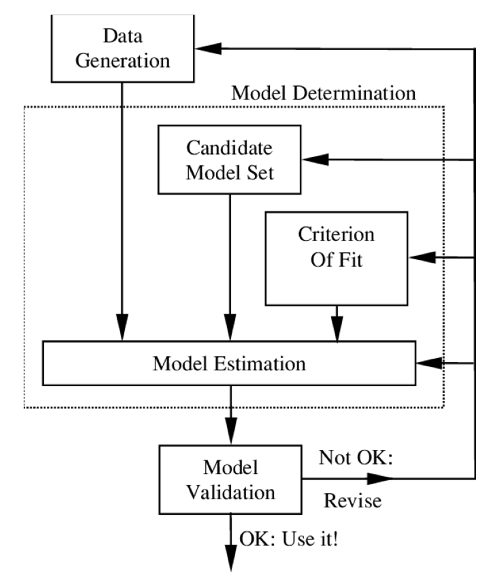
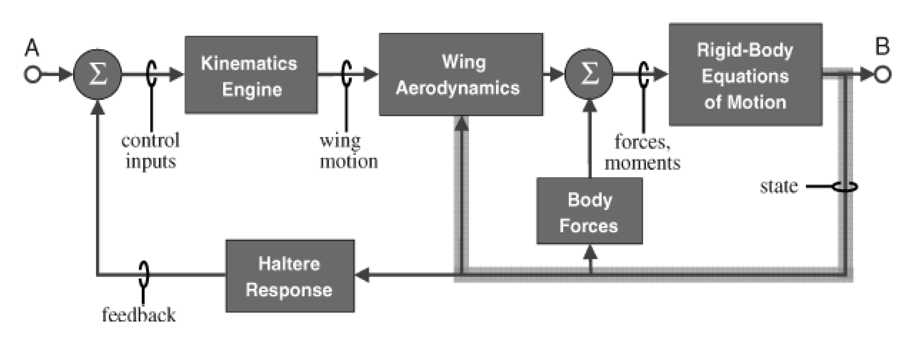
Table 1.
Average and standard deviation of the estimated parameters for the full and reduced order models [93].
Table 1.
Average and standard deviation of the estimated parameters for the full and reduced order models [93].
| Model | Force | ||||||||||||||||
|---|---|---|---|---|---|---|---|---|---|---|---|---|---|---|---|---|---|
| Mom-ent | Avg | Std. Dev. | Avg | Std. Dev. | Avg | Std. Dev. | Avg | Std. Dev. | Avg | Std. Dev. | Avg | Std. Dev. | Avg | Std. Dev. | Avg | Std. Dev. | |
| Full | X | 0.1538 | 0.1131 | 0.0110 | 0.0194 | 0.0483 | 0.0431 | −0.0100 | 0.0221 | −0.049 | 0.0246 | −0.1095 | 0.1114 | −0.0027 | 0.0358 | 5.4100E-4 | 0.0018 |
| Y | 0.0225 | 0.028 | 0.0055 | 0.0316 | −0.0205 | 0.0245 | −0.0274 | 0.0006 | 8.9522E-4 | 0.0169 | −0.0614 | 0.0540 | −0.0158 | 0.0331 | −0.0073 | 0.0029 | |
| Z | −0.2861 | 0.0297 | −0.0097 | 0.0132 | 0.1699 | 0.0168 | −0.0030 | 0.0094 | 0.0014 | 0.0084 | −0.0134 | 0.0478 | −0.0047 | 0.0121 | −4.4929E-4 | 0.0007 | |
| L | 9.6231E-4 | 0.0004 | −8.426E-5 | 2.970E-5 | −6.9285E-4 | 0.0002 | 1.4884E-5 | 3.660E-5 | −1.8120E-4 | 0.0006 | 7.9049E-5 | 0.0004 | −6.1030E-4 | 0.0007 | −2.1300E-5 | 5E-6 | |
| M | 0.0414 | 0.0191 | 0.0033 | 0.0056 | −0.0203 | 0.0078 | 0.0041 | 0.0019 | −0.0054 | 0.0044 | 0.0014 | 0.0084 | −0.0144 | 0.0059 | −0.0021 | 0.0006 | |
| N | −0.088 | 0.0134 | −0.0017 | 0.0012 | 0.0011 | 0.0047 | −4.3412E-4 | 0.0011 | −2.2278E-4 | 0.01678 | −0.0155 | 0.0166 | 0.0011 | 0.0269 | 1.2782E-4 | 0.0002 | |
| X | 0.0067 | 0.0024 | 0.0067 | 0.0093 | 0.0108 | 0.0019 | −0.1252 | 0.0430 | 0.0829 | 0.0037 | −0.0035 | 0.0160 | 0.0039 | 0.1243 | |||
| Y | 3.6187E-4 | 0.0014 | −0.0014 | 0.0091 | 0.0265 | 0.0244 | 0.0124 | 0.0237 | 0.0018 | 0.0008 | −0.0011 | 0.0021 | 0.021 | 0.0008 | |||
| Z | −0.0018 | 0.0010 | −0.0051 | 0.0049 | −0.0065 | 0.0005 | 0.0519 | 0.0240 | −0.0100 | 0.0013 | 4.2333E-4 | 0.0081 | −0.0012 | 0.0343 | |||
| L | 7.4992E-5 | 5.16E-5 | 1.358E-5 | 7.86E-6 | 1.9198E-4 | 0.0007 | 1.0647E-4 | 0.0004 | −7.0396E-5 | 1.18E-6 | 6.5270E-6 | 8.14E-5 | −5.5306E-6 | 2.118E-5 | |||
| M | 0.0013 | 0.0005 | 5.516E-4 | 0.0014 | −6.6045E-4 | 0.0002 | −0.0478 | 0.0181 | 5.1973E-4 | 0.0007 | −3.1036E-4 | 0.0035 | −1.6626E-4 | 0.0148 | |||
| N | 2.7412E-4 | 0.0008 | −0.0019 | 0.0003 | 1.9530E-4 | 0.0245 | 0.0280 | 0.0162 | 0.0033 | 0.0003 | 4.2332E-4 | 0.0032 | −2.4090E-4 | 0.0011 | |||
| Reduced | X | 0.1385 | 0.0254 | 0.0354 | 0.0007 | ||||||||||||
| Y | −0.0353 | 0.0184 | −0.0412 | 0.0231 | −0.007 | 0.0019 | |||||||||||
| Z | −0.2437 | 0.0224 | 0.1650 | 0.0022 | |||||||||||||
| L | 1.0851E-5 | 0.0001 | 9.1882E-6 | 3.66E-5 | |||||||||||||
| M | −0.0067 | 0.0191 | −0.0031 | 0.0032 | |||||||||||||
| N | 0.0016 | 0.0057 | −7.1896E-4 | 0.0016 | |||||||||||||
| . | |||||||||||||||||
| 0.055 | 0.0009 | −0.017 | 0.0019 | 0.0093 | 0.0023 | ||||||||||||
| Y | 0.0028 | 0.0015 | −0.0059 | 0.0077 | |||||||||||||
| Z | 0.0016 | 0.0014 | −0.0012 | 0.0019 | −0.0055 | 0.0024 | |||||||||||
| L | −4.0721E-6 | 5.26E-6 | −5.9233E-4 | 6.68E-6 | |||||||||||||
| M | 8.007E-4 | 0.018 | 0.0023 | 0.0039 | |||||||||||||
| N | 2.7054E-5 | 0.0003 | 0.0208 | 0.0004 | |||||||||||||
Table 2.
This indicates the estimated stability and control derivatives [143].
Table 2.
This indicates the estimated stability and control derivatives [143].
| Parameter | Value | Standard Deviation |
|---|---|---|
| Xu | −12.3 | 4.0% |
| Zw | −4.7 | 9.1% |
| Mu | 547 | 3.6% |
| −33.3 | 4.6% | |
| 12.7 | 12.2% | |
| 20.7 | 7.6% | |
| −17.4 | 4.8% | |
| 6028 | 3.6% | |
| −2826 | 3.8% | |
| −12360 | 5.0% | |
| −87.74 | 10.7% |
Publisher’s Note: MDPI stays neutral with regard to jurisdictional claims in published maps and institutional affiliations. |
© 2021 by the authors. Licensee MDPI, Basel, Switzerland. This article is an open access article distributed under the terms and conditions of the Creative Commons Attribution (CC BY) license (http://creativecommons.org/licenses/by/4.0/).
Share and Cite
MDPI and ACS Style
Khan, Q.; Akmeliawati, R. Review on System Identification and Mathematical Modeling of Flapping Wing Micro-Aerial Vehicles. Appl. Sci. 2021, 11, 1546. https://0-doi-org.brum.beds.ac.uk/10.3390/app11041546
AMA Style
Khan Q, Akmeliawati R. Review on System Identification and Mathematical Modeling of Flapping Wing Micro-Aerial Vehicles. Applied Sciences. 2021; 11(4):1546. https://0-doi-org.brum.beds.ac.uk/10.3390/app11041546
Chicago/Turabian StyleKhan, Qudrat, and Rini Akmeliawati. 2021. "Review on System Identification and Mathematical Modeling of Flapping Wing Micro-Aerial Vehicles" Applied Sciences 11, no. 4: 1546. https://0-doi-org.brum.beds.ac.uk/10.3390/app11041546
Note that from the first issue of 2016, this journal uses article numbers instead of page numbers. See further details here.